Flood Modeling Using a Synthesis of Multi-Platform LiDAR Data


Abstract
:
1. Introduction
2. Data and Methods
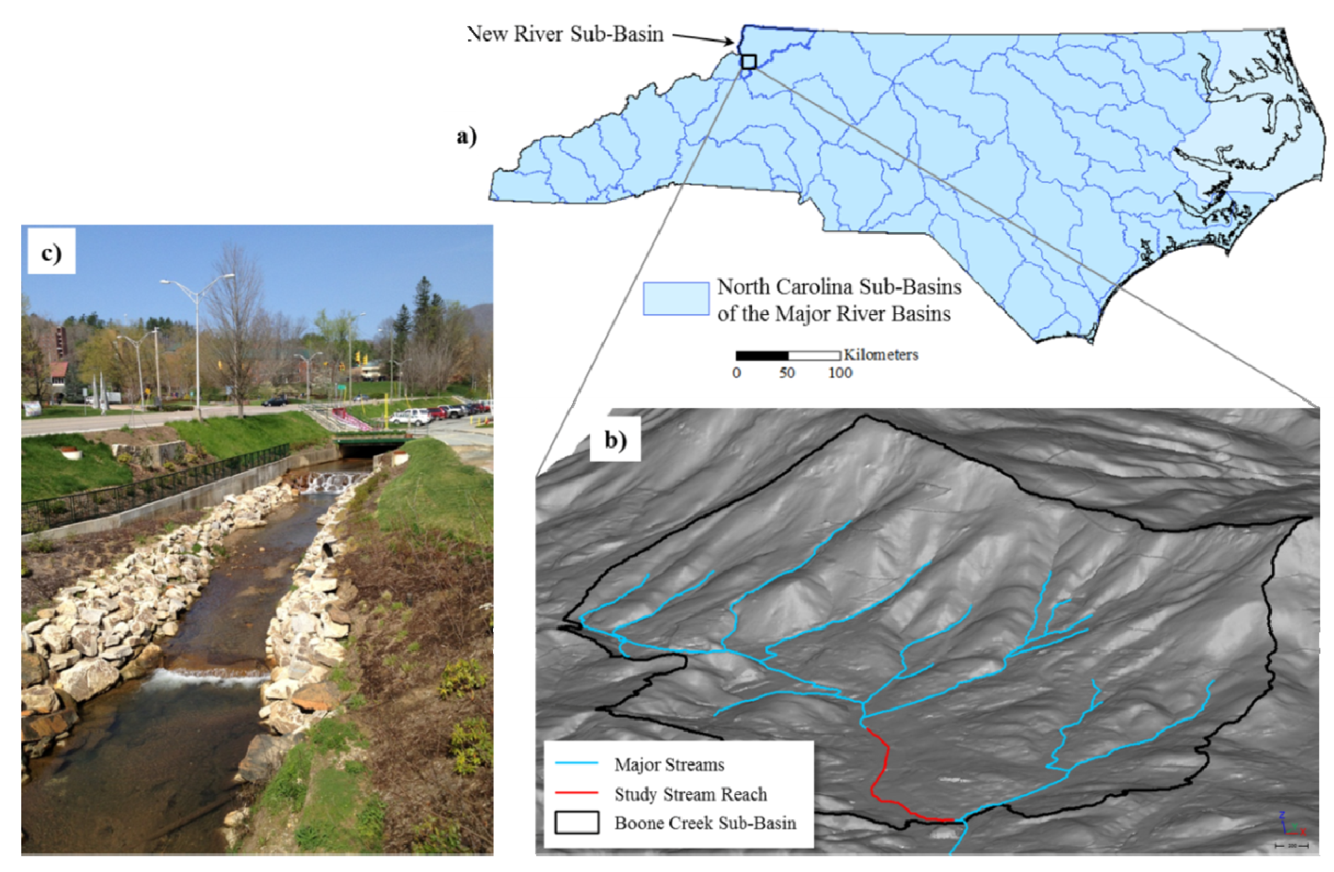
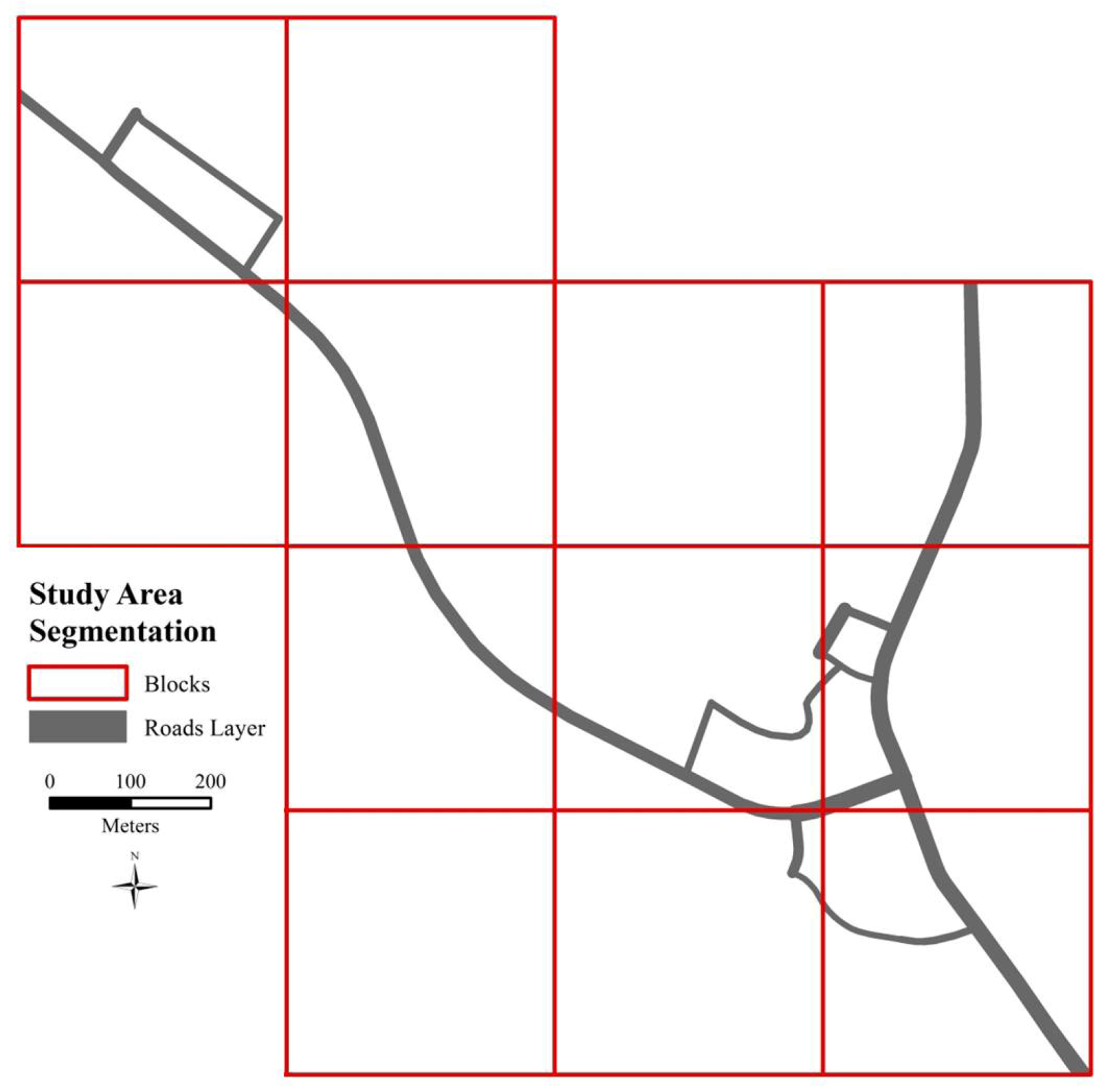
2.1. Study Area

2.2. Airborne LiDAR Data Acquisition and Processing

| Descriptions | Airborne | Mobile | Terrestrial |
|---|---|---|---|
| Scanner system | Leica Geosystems Aeroscan | Trimble MX8 Pod | Leica ScanStation C10 |
| Range | Flown 3050 m AGL | 200 m | 300 m |
| Vertical RMSE | 25 cm | 6 cm | 3 cm |
| Measurement rate | 150 kHz | 300 kHz | 50 kHz |
| Field-of-view | 55° | 360° | 360° (horizontal); 270° (vertical) |
| Nominal all-return point-spacing | 5 m | 0.05 m | 0.005 m |
| Acquisition date | March 2003 | July 2011 | July 2011 |
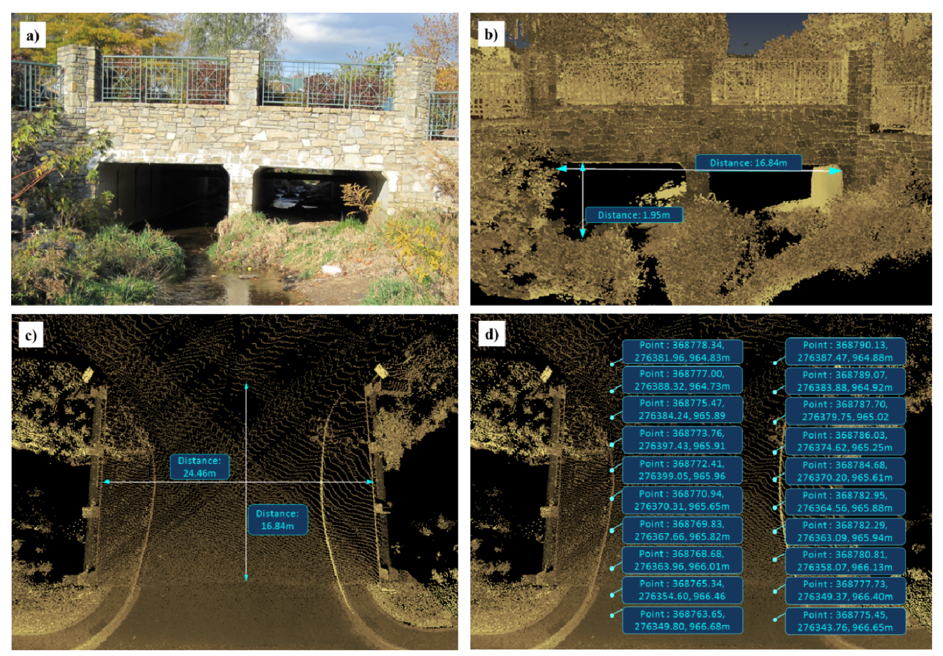
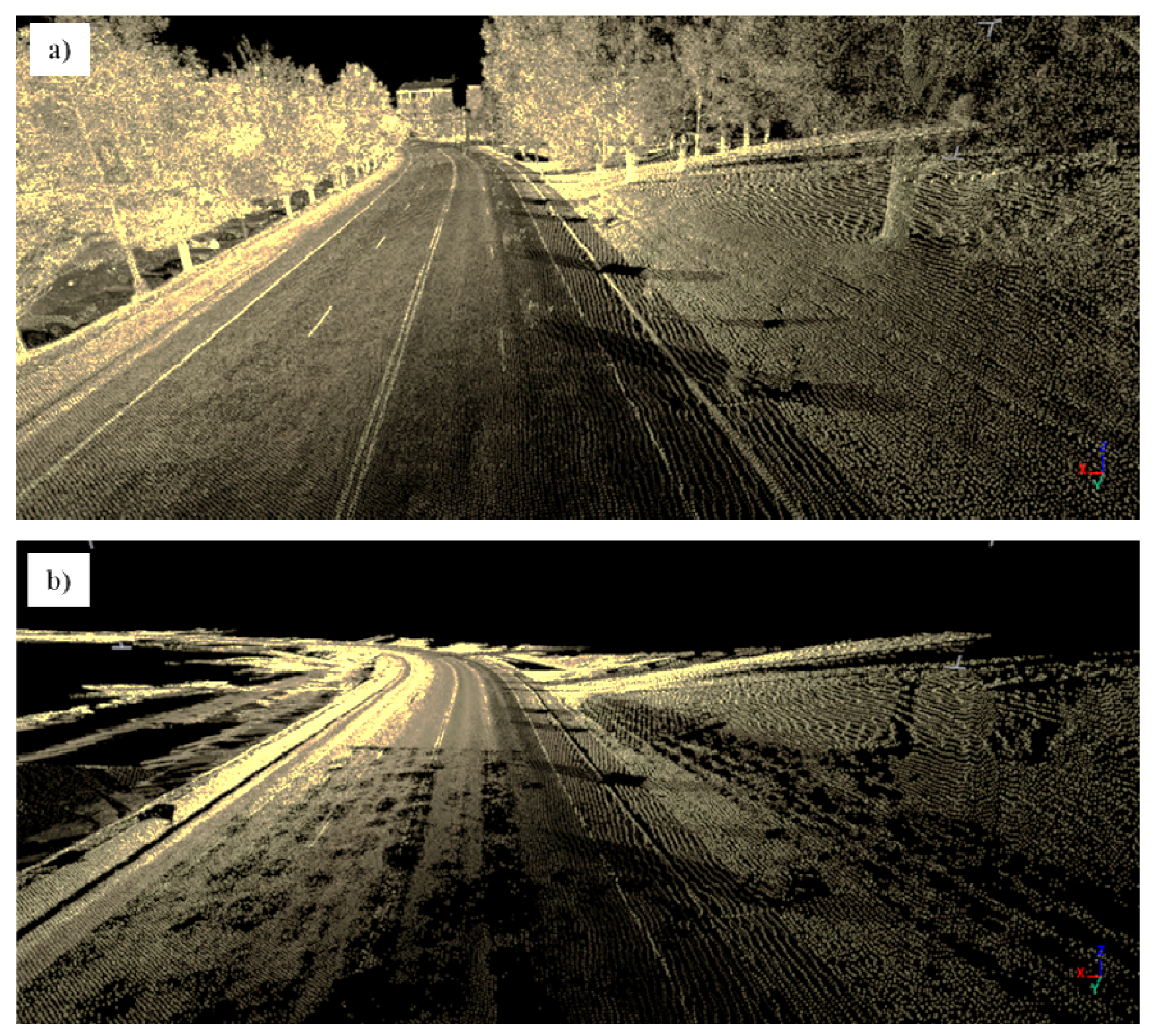
2.3. Ground-Based LiDAR Data Acquisition and Processing
2.3.1. Mobile LiDAR
2.3.2. Terrestrial LiDAR
2.3.3. Ground Control Points and the Continuously Operating Reference Station
2.3.4. Mobile and Terrestrial LiDAR Post-Processing
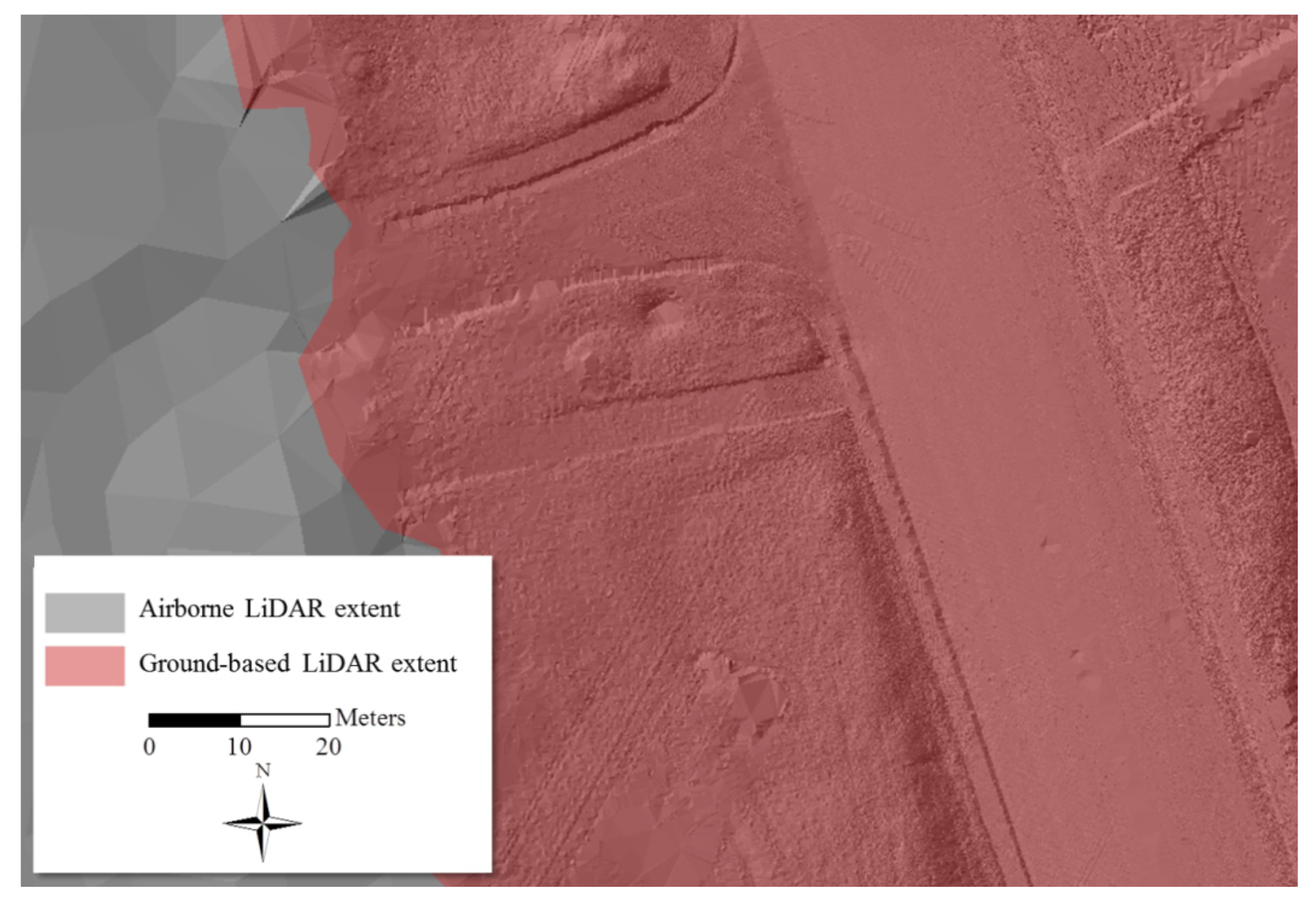
2.3.5. Synthesis of Airborne and Ground-Based Bare-Earth LiDAR Data and TIN Generation
2.4. LiDAR Data Quality in the U.S.
2.5. LiDAR Accuracy Assessments
2.6. Flood Modeling
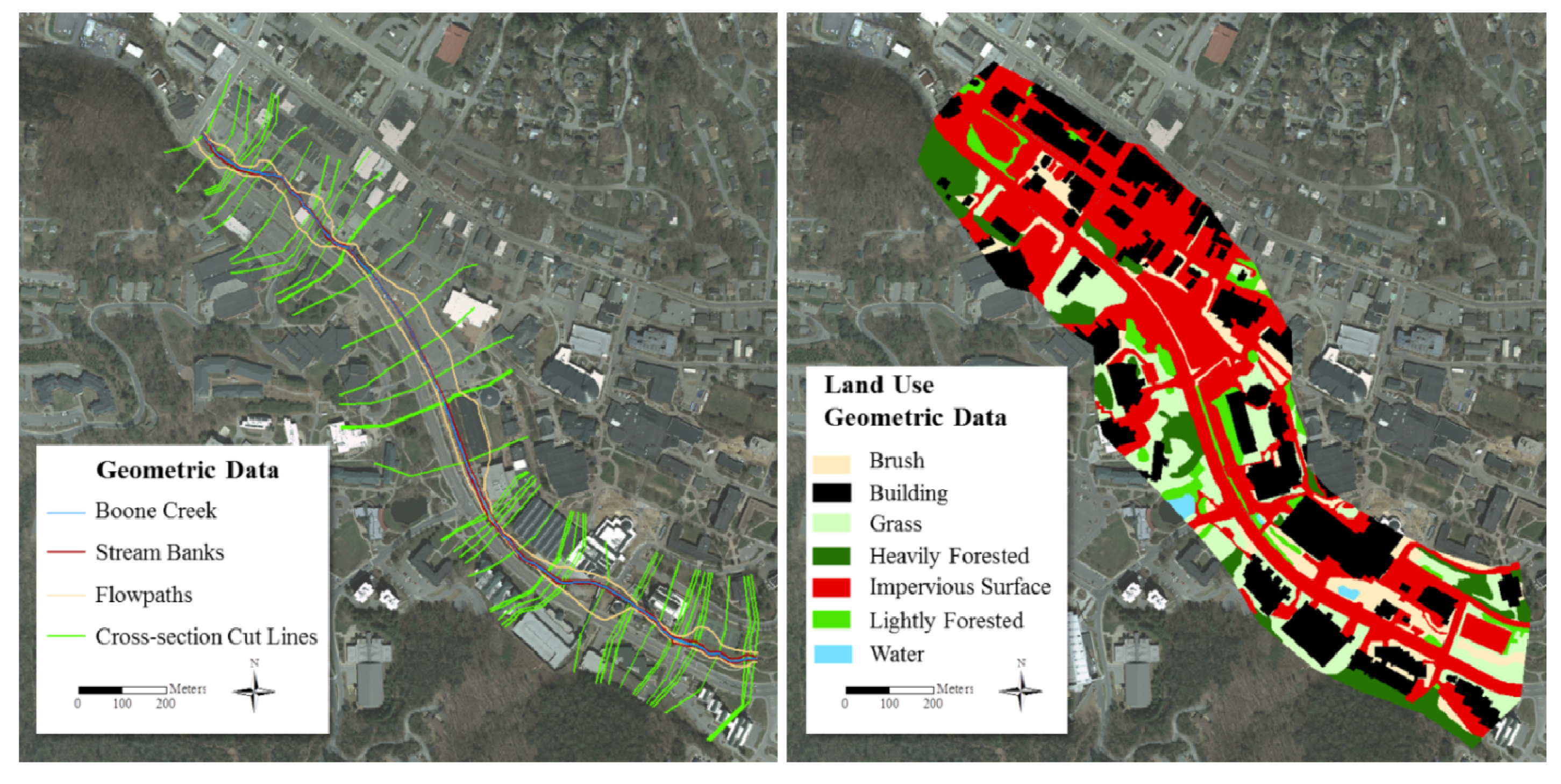
2.6.1. Input Data
2.6.2. Flood Modeling Using HEC-RAS and ArcGIS


2.6.3. Flood Modeling Diagnostics

3. Results and Discussion
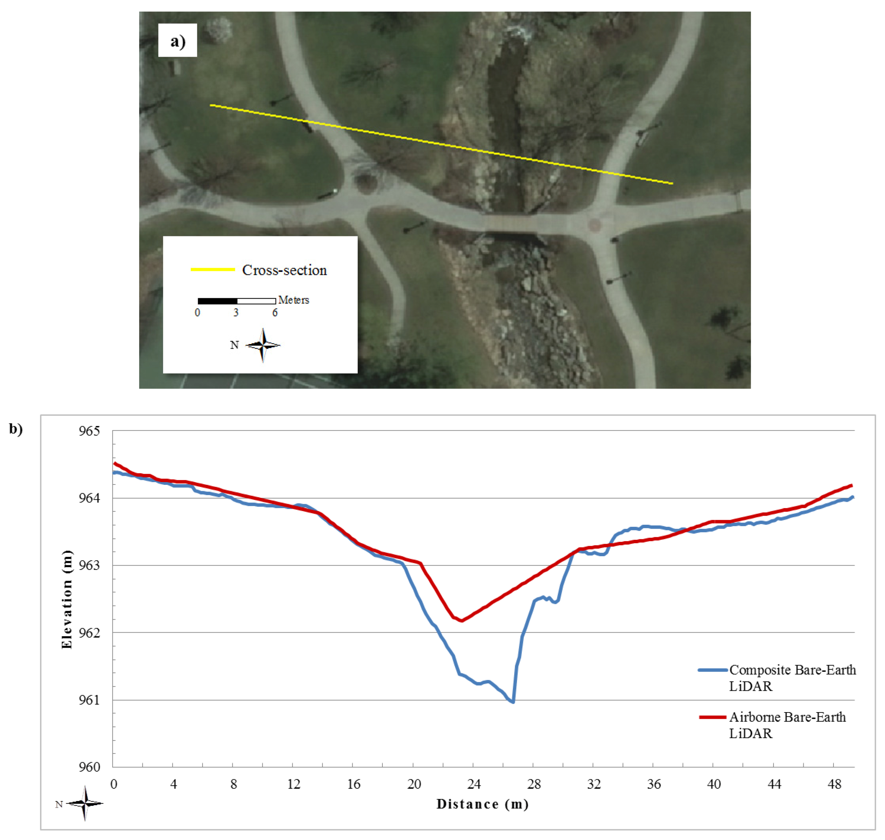
3.1. Bare-Earth LiDAR Accuracy Assessment and Comparison
| Statistics | GCP minus Airborne | GCP minus Composite |
|---|---|---|
| Mean Difference [abs]* (m) | 0.133 | 0.081 |
| Maximum Difference (m) | 0.800 | 0.616 |
| Range (m) | 0.962 | 0.619 |
| Standard Deviation | 0.193 | 0.145 |
| Statistics | Pavement | Grass | Slope |
|---|---|---|---|
| Mean Difference [abs] (m) | 0.074 | 0.068 | 0.230 |
| Maximum Difference (m) | 0.215 | 0.228 | 1.416 |
| Range (m) | 0.239 | 0.451 | 2.013 |
| Standard Deviation | 0.071 | 0.099 | 0.412 |
| Statistics | Airborne minus Composite Elevation Values |
|---|---|
| Mean Difference [abs] (m) | 0.178 |
| Maximum Difference (m) | 1.677 |
| Range (m) | 2.730 |
| Standard Deviation | 0.335 |
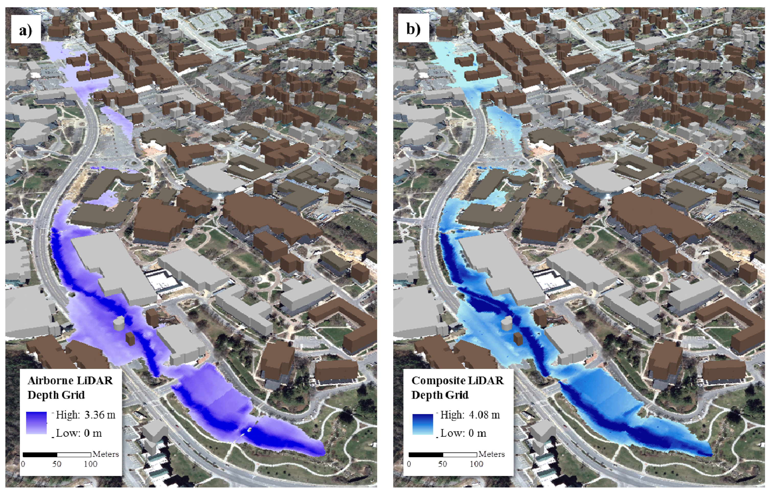
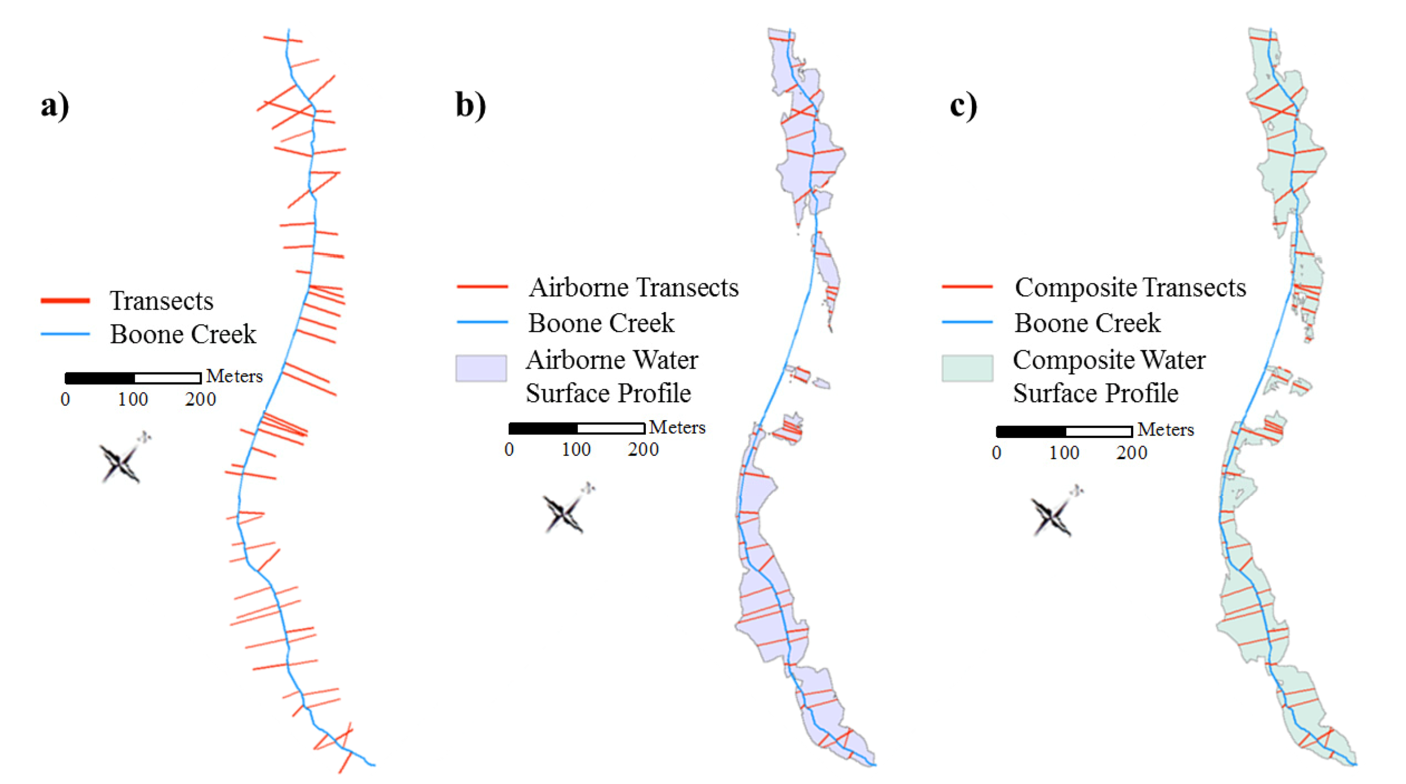
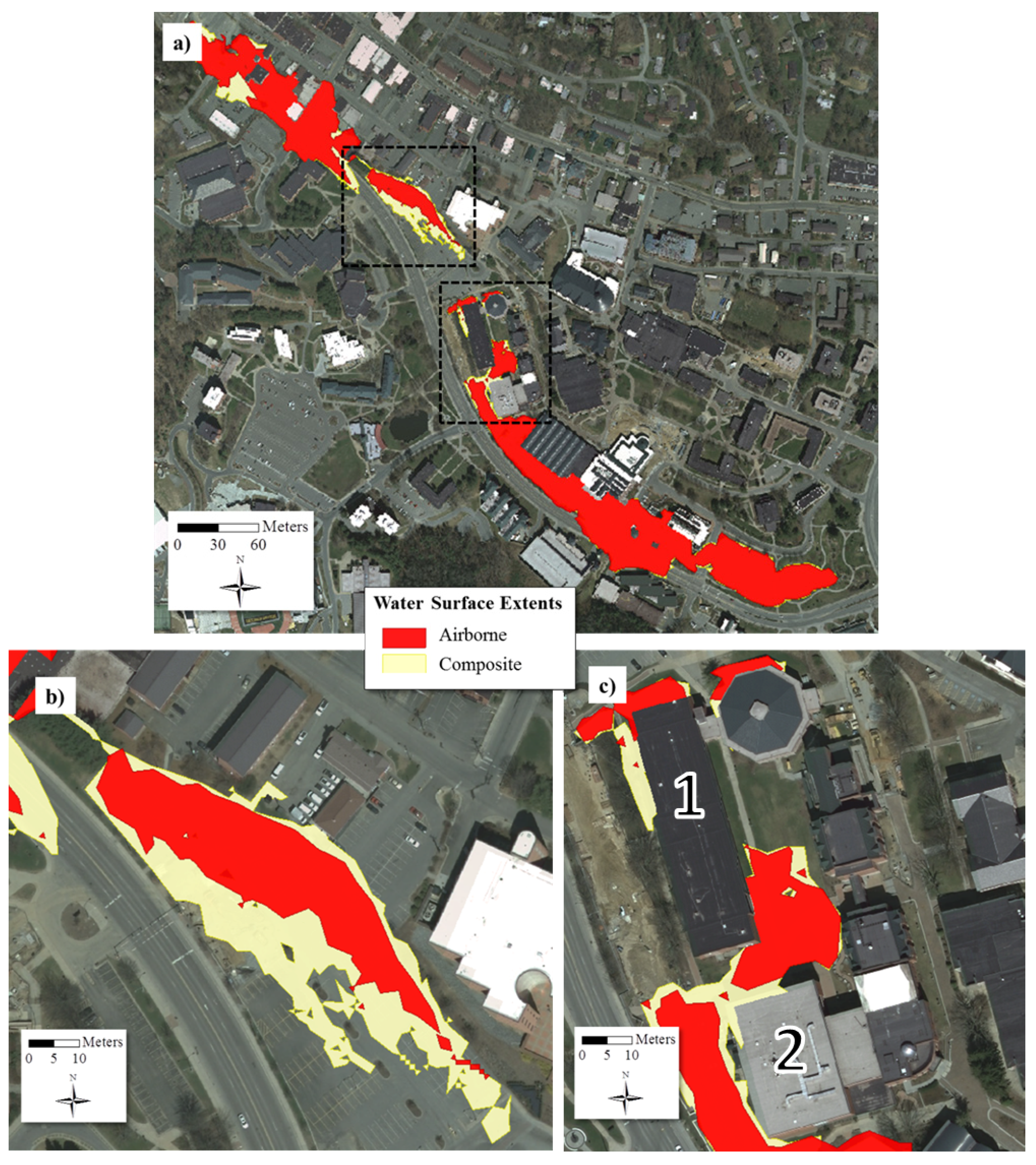
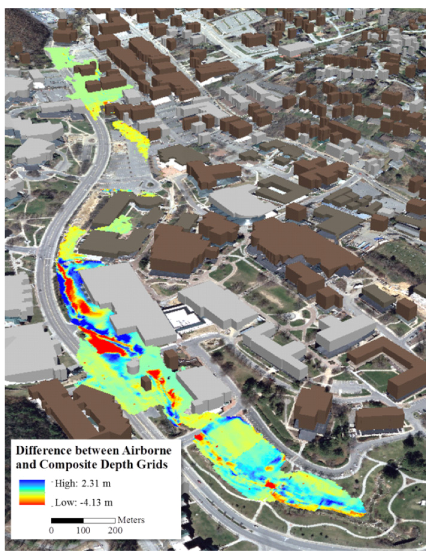
3.2. Flood Modeling Results
| Statistics | Airborne | Composite | Percent Different |
|---|---|---|---|
| Area (m2) | 55,238.94 | 59,887.62 | 8.08% |
| Average Transect Distance Flooded (m) | 25.59 | 28.44 | 10.55% |
| Mean Percentage of Transects Flooded | 48.36 | 51.98 | 7.22% |
| Symmetric Difference (Error %) between Water Surface Profiles | 17.76% | ||
| Parametric Paired-T Test p-value (at 0.05 significance level) | 0.039 | ||

| Statistics | Airborne | Composite | Percent Different |
|---|---|---|---|
| Volume (m3) | 28,800.51 | 29,696.98 | 3.06% |
| Maximum Flood Height (m) | 3.36 | 4.81 | 35.37% |
| Root Mean Squared Error (RMSE) between Airborne and Composite | 1.36 m | ||
4. Conclusions and Future Research
Acknowledgements
Conflicts of Interest
References
- White, G.F. Human Adjustment to Floods: A Geographical Approach to the Flood Problem in the United States; Research Paper No. 29; University of Chicago, Department of Geography: Chicago, IL, USA, 1942. [Google Scholar]
- National Research Council of the National Academies. 1: Introduction. In Mapping the Zone: Improving Flood Map Accuracy; The National Academies Press: Washington, DC, USA, 2009; pp. 1–12. [Google Scholar]
- Wohl, E.E. Chapter 1: Inland flood hazards. In Inland Flood Hazards: Human, Riparian, and Aquatic Communities; Wohl, E.E., Ed.; Cambridge University Press: New York, NY, USA, 2011; pp. 3–36. [Google Scholar]
- European Commission. A New EU Floods Directive. Available online: http://ec.europa.eu/environment/water/flood_risk/ (accessed on 29 July 2013).
- Mark, O.; Weesakul, S.; Apirumanekul, C.; Aroonnet, S.B.; Djordjevic, S. Potential and limitations of 1D modeling of urban flooding. J. Hydrol. 2004, 299, 284–299. [Google Scholar]
- Yu, D.; Lane, S.N. Urban fluvial flood modeling using a two-dimensional diffusion-wave treatment, Part 2: Development of a sub-grid-scale treatment. Hydrol. Process. 2006, 20, 1567–1583. [Google Scholar] [CrossRef]
- Bates, P. Remote sensing and flood inundation modelling. Hydrol. Process. 2004, 18, 2539–2597. [Google Scholar]
- Hollaus, M.; Wagner, W.; Kraus, K. Airborne laser scanning and usefulness for hydrological models. Adv. Geosci. 2005, 5, 57–63. [Google Scholar] [CrossRef]
- Bremer, M.; Sass, O. Combining airborne and terrestrial laser scanning for quantifying erosion and deposition by a debris flow event. Geomorphology 2012, 128, 49–60. [Google Scholar] [CrossRef]
- Hunter, N.; Bates, P.; Neelz, S.; Pender, G.; Villanueva, I.; Wright, N.; Liang, D.; Falconer, R.; Lin, B.; Waller, S.; et al. Benchmarking 2D hydraulic models for urban flooding. Water Manag. 2008, 161, 13–30. [Google Scholar]
- McMillan, H.; Brasington, J. Reduced complexity strategies for modelling urban floodplain inundation. Geomorphology 2009, 90, 226–243. [Google Scholar] [CrossRef]
- Vojinovic, Z; Tutulic, D. On the use of 1D-2D modelling approaches for assessment of flood damage in urban areas. Urban Water J. 2009, 6, 183–199. [Google Scholar] [CrossRef]
- Haile, A.T.; Rientjes, T.H.M. Effects of LiDAR DEM Resolution in Flood Modelling: A Model Sensitivity Study for the City of Tegucigalpa, Honduras; ISPRS WG III/3, III/4, V/3 Workshop: Enschede, The Netherlands, 2005; pp. 169–173. [Google Scholar]
- Fewtrell, T.J.; Duncan, A.; Sampson, C.C.; Neal, J.C.; Bates, P.D. Benchmarking urban flood models of varying complexity and scale using high resolution terrestrial LiDAR data. Phys. Chem. Earth 2011, 36, 281–291. [Google Scholar] [CrossRef]
- Sampson, C.; Bates, P.; Duncan, A.; Fewtrell, T. Merging Airborne and Terrestrial LiDAR Data to Determine Geometric Controls on Flood Propagation in Urban Areas; EGU2011-13739; European Geoscience Union General Assembly: Vienna, Austria, 2011.
- Brasington, J.; Vericat, D.; Rychkov, I. Modeling river bed morphology, roughness, and surface sedimentology using high resolution terrestrial laser scanning. Water Resour. Res. 2012, 48. [Google Scholar] [CrossRef]
- Hoshenthal, J.; Alho, P.; Hyyppa, J.; Hyyppa, H. Laser scanning applications in fluvial studies. Prog. Phys. Geogr. 2011, 35, 782–809. [Google Scholar] [CrossRef]
- Wehr, A. Airborne laser scanning—An introduction and overview. ISPRS J. Photogramm. Remote Sens. 1999, 54, 68–82. [Google Scholar] [CrossRef]
- Dewberry. Final Report of the National Enhanced Elevation Assessment; Dewberry: Fairfax, VA, USA, 2011; (revised 2012); Available online: http://www.dewberry.com/files/pdf/NEEA_Final%20Report_Revised%203.29.12.pdf (accessed on 29 June 2013).
- National Research Council. Elevation data for floodplain mapping; The National Academies Press: Washington, DC, USA, 2007. [Google Scholar]
- Merwade, V.; Olivera, F.; Arabi, M.; Edleman, S. Uncertainty in flood inundation mapping: Current issues and future directions. J. Hydrol. Eng. 2008, 13, 608–620. [Google Scholar] [CrossRef]
- Marks, K.; Bates, P.D. Integration of high-resolution topographic data with floodplain flow models. Hydrol. Process. 2000, 14, 2109–2122. [Google Scholar] [CrossRef]
- Manson, S.M.; Ratick, S.J.; Solow, A.R. Decision making and uncertainty: Bayesian analysis of potential flood heights. Geogr. Anal. 2002, 34, 112–129. [Google Scholar]
- Omer, C.R.; Nelson, E.J.; Zundel, A.K. Impact of varied data resolution on hydraulic modeling and floodplain delineation. J. Am. Water Resour. Assoc. 2003, 39, 467–475. [Google Scholar] [CrossRef]
- Casas, A.; Benito, G.; Thorndycraft, V.R.; Rico, M. The topographic data source of digital terrain models as a key element in the accuracy of hydraulic flood modeling. Earth Surf. Process. Landf. 2006, 31, 444–456. [Google Scholar] [CrossRef]
- Cook, A.; Merwade, V. Effect of topographic data, geometric configuration and modeling approach on flood inundation mapping. J. Hydrol. 2009, 377, 131–142. [Google Scholar] [CrossRef]
- Fewtrell, T.J.; Bates, P.D.; Horritt, M.; Hunter, N.M. Evaluating the effect of scale in flood inundation modelling in urban environments. Hydrol. Process. 2008, 22, 5107–5118. [Google Scholar] [CrossRef]
- Gallegos, H.A.; Schubert, J.E.; Sanders, B.F. Two-dimensional, high-resolution modeling of urban dam-break flooding: A case study of Baldwin Hills, California. Adv. Water Resour. 2009, 32, 1323–1335. [Google Scholar] [CrossRef]
- Webster, T. Flood risk mapping using LiDAR for Annapolis Royal, Nova Scotia, Canada. Remote Sens. 2010, 2, 2060–2082. [Google Scholar] [CrossRef]
- Marcus, W.A.; Aspinall, R.J.; Marston, R.A. Geographic Information Systems and Surface Hydrology. In Geographic Information Science and Mountain Geomorphology; Bishop, M.P., Shroder, J.F., Jr., Eds.; Springer: New York, NY, USA, 2005; pp. 343–379. [Google Scholar]
- Colby, J.D.; Dobson, J.G. Flood modeling in the coastal plains and mountains: Analysis of terrain resolution. Nat. Hazards Rev. 2010, 11, 19–28. [Google Scholar] [CrossRef]
- Iavarone, A.; Vagners, D. Sensor fusion: Generating 3D by combining airborne and tripod-mounted LIDAR data. In Proceedings of the International Workshop on Visualization and Animation of Reality-Based 3D Models 2003, International Archives of the Photogrammetry, Remote Sensing and Spatial Information Sciences, Engadin, Switzerland, 24–28 February 2003; Volume 34-5/W10.
- Böhm, J.; Haala, N. Efficient Integration of Aerial and Terrestrial Laser Data for Virtual City Modeling Using LASERMAPS; ISPRS Volume 36 Part 3/W19; ISPRS Workshop Laser Scanning: Enschede, The Netherlands, 2005; pp. 192–197. [Google Scholar]
- Van Leeuwen, M.; Hilker, T.; Coops, N.C.; Frazer, G.W.; Wulder, M.A.; Newnham, G.J.; Culvenor, D.S. Assessment of standing wood and fiber quality using ground and airborne laser scanning: A review. For. Ecol. Manag. 2011, 261, 1467–1478. [Google Scholar] [CrossRef]
- Kasvi, E.; Vaaja, M.; Alho, P.; Hyyppa, H.; Hyyppa, J.; Kaartinen, H.; Kukko, A. Morphological changes on meander bars associated with flow structure at different discharges. Earth Surf. Process. Landf. 2013, 38, 577–590. [Google Scholar] [CrossRef]
- Methods, H.; Dyhouse, G.; Hatchett, J.; Benn, J. Chapter 6: Bridge Modeling. In Floodplain Modeling Using HEC-RAS, 1st ed.; Totz, C., Klotz, D., Strafaci, A., Hogan, A., Dietrich, K., Eds.; Haestad Press: Waterbury, CT, USA, 2003; pp. 167–231. [Google Scholar]
- Methods, H.; Dyhouse, G.; Hatchett, J.; Benn, J. Chapter 7: Culvert Modeling. In Floodplain Modeling Using HEC-RAS, 1st ed.; Totz, C., Klotz, D., Strafaci, A., Hogan, A., Dietrich, K., Eds.; Haestad Press: Waterbury, CT, USA, 2003; pp. 233–281. [Google Scholar]
- Chang, J.; Tsai, M.; Findley, D.; Cunningham, C. North Carolina Department of Transportation Research Project No. 2012-15: Infrastructure Investment Protection with LiDAR; FHWA/NC/2012-15; North Carolina Department of Transportation Research and Analysis Group: Raleigh, NC, USA, 2012; pp. 1–84. [Google Scholar]
- Pielke, R.A., Jr.; Downton, M.W.; Miller, J.Z.B. Flood Damage in the United States, 1926–2000: A Reanalysis of National Weather Service Estimates; University Corporation for Atmospheric Research (UCAR): Boulder, CO, USA, 2002; pp. 1–86. [Google Scholar]
- Bales, J.D.; Wagner, C.R.; Tighe, K.C.; Terziotti, S. LiDAR-Derived Flood-Inundation Maps for Real-Time Flood-Mapping Applications, Tar River basin, North Carolina; U.S. Geological Survey Scientific Investigations Report 2007-5032; U.S. Geological Survey: Reston, VA, USA, 2007; pp. 1–52.
- Coffey, C. The Effects of Impervious Surfaces and Forests on Water Quality in a Southern Appalachian Headwater Catchment: A Geospatial Modeling Approach. Master’s Thesis, Appalachian State University, Boone, NC, USA, August 2011. [Google Scholar]
- Wohl, E.E. Mountain Rivers, Water Resources Monograph; American Geophysical Union: Washington, DC, USA, 2000; Volume 14, pp. 1–320. [Google Scholar]
- Anderson, W.P.; Anderson, J.L.; Thaxton, C.S.; Babyak, C.M. Changes in stream temperatures in response to restoration of groundwater discharge and solar heating in a culverted, urban stream. J. Hydrol. 2010, 393, 309–320. [Google Scholar] [CrossRef]
- NC Geographic Information Coordinating Council. NC OneMap, Discover/Get Geospatial Data. Available online: http://www.nconemap.com/DiscoverGetData.aspx (accessed on 1 May 2012).
- State Climate Office of North Carolina. Overview. Available online: http://www.nc-climate.ncsu.edu/climate/ncclimate.html (accessed on 20 March 2012).
- Floodplain Mapping Program, North Carolina Division of Emergency Management. In NC Floodplain Mapping: Watauga River Basin; LiDAR Bare Earth Mass Points, Feb-Apr and Dec 2003; EarthData International of North Carolina: High Point, NC, USA, 2004; Available online: http://floodmaps.nc.gov/fmis/Download.aspx?FIPS=189 (accessed on 1 October 2011).
- North Carolina Floodplain Mapping Program. Floodplain Mapping Information System. Available online: http://floodmaps.nc.gov/fmis/Download.aspx (accessed on 1 September 2011).
- National Geodetic Survey. Continuously Operating Reference Station (CORS). Available online: http://geodesy.noaa.gov/CORS/ (accessed on 1 September 2011).
- Applanix Corp. POSPac Mobile Mapping Suite. Available online: http://www.applanix.com/products/land/pospac-mms.html (accessed on 1 October 2011).
- Axelsson, P. Processing of laser scanner data—Algorithms and applications. ISPRS J. Photogramm. Remote Sens. 1999, 54, 138–137. [Google Scholar] [CrossRef]
- U.S. Geological Survey (USGS). Endorsement for a 3D Elevation Program by the National Digital Elevation Program (NDEP). Available online: http://nationalmap.gov/3DEP/documents/ndep_endorsement_dec2012.pdf (accessed on 25 June 2013).
- Methods, H.; Dyhouse, G.; Hatchett, J.; Benn, J. Chapter 1: Introduction to Floodplain Modeling and Management. In Floodplain Modeling Using HEC-RAS, 1st ed.; Totz, C., Klotz, D., Strafaci, A., Hogan, A., Dietrich, K., Eds.; Haestad Press: Waterbury, CT, USA, 2003; pp. 167–231. [Google Scholar]
- US Army Corps of Engineers. HEC-RAS River Analysis System, User’s Manual; U.S. Army Corps of Engineers, Hydrologic Engineering Center, Institute for Water Resources: Davis, CA, USA; p. 2010.
- Johnson, L.E. 9: GIS for Floodplain Management. In Geographic Information Systems in Water Resource Engineering; Taylor and Francis, LLC: Boca Raton, FL, USA, 2009; pp. 187–206. [Google Scholar]
- Federal Emergency Management Agency State of North Carolina. Flood Insurance Study: A Report of Flood Hazards in Watauga County, North Carolina and Incorporated Areas; FEMA: Atlanta, GA, USA, 2009; pp. 1–218. [Google Scholar]
- US Army Corps of Engineers. HEC-GeoRAS. Available online: http://www.hec.usace.army.mil/software/hec-georas (accessed on 1 June 2011).
- Chow, V.T. Open-Channel Hydraulics; McGraw-Hill Book Co., Inc.: New York, NY, USA, 1959. [Google Scholar]
- US Army Corps of Engineers (USACE); Hydrologic Engineering Center. HEC-RAS River Analysis System: Hydraulic Reference Manual; Version 4.1; USACE: Davis, CA, USA, 2010. [Google Scholar]
- Gueudet, P.; Wells, G.; Maidment, D.; Neuenschwander, A. Influence of the post-spacing of the LiDAR-derived DEM on flood modeling. In Proceedings of 2004 American Water Resources Association Spring Specialty Conference, GIS and Water Resources III, Nashville, TN, USA, 17 May 2004; pp. 1–5.
- Wang, Y.; Zheng, T. Comparison of light detection and ranging and nation elevation dataset digital elevation model on floodplains of North Carolina. Nat. Hazards Rev. 2005, 6, 34–40. [Google Scholar] [CrossRef]
- Li, J.; Wong, D.W.S. Effects of DEM sources on hydrologic applications. Comput. Environ. Urban Syst. 2010, 34, 251–261. [Google Scholar] [CrossRef]
- Abdullah, A.F.; Vojinovic, Z.; Price, R.K.; Aziz, N.A.A. A methodology for processing raw LiDAR data to support urban flood modelling framework. J. Hydroinforma. 2012, 14, 75–92. [Google Scholar] [CrossRef]
© 2013 by the authors; licensee MDPI, Basel, Switzerland. This article is an open access article distributed under the terms and conditions of the Creative Commons Attribution license (http://creativecommons.org/licenses/by/3.0/).
Share and Cite
Turner, A.B.; Colby, J.D.; Csontos, R.M.; Batten, M. Flood Modeling Using a Synthesis of Multi-Platform LiDAR Data. Water 2013, 5, 1533-1560. https://doi.org/10.3390/w5041533
Turner AB, Colby JD, Csontos RM, Batten M. Flood Modeling Using a Synthesis of Multi-Platform LiDAR Data. Water. 2013; 5(4):1533-1560. https://doi.org/10.3390/w5041533
Chicago/Turabian StyleTurner, Ashleigh B., Jeffrey D. Colby, Ryan M. Csontos, and Michael Batten. 2013. "Flood Modeling Using a Synthesis of Multi-Platform LiDAR Data" Water 5, no. 4: 1533-1560. https://doi.org/10.3390/w5041533
APA StyleTurner, A. B., Colby, J. D., Csontos, R. M., & Batten, M. (2013). Flood Modeling Using a Synthesis of Multi-Platform LiDAR Data. Water, 5(4), 1533-1560. https://doi.org/10.3390/w5041533