Inundation Mapping Initiatives of the Iowa Flood Center: Statewide Coverage and Detailed Urban Flooding Analysis

Abstract
:
1. Introduction

2. Background
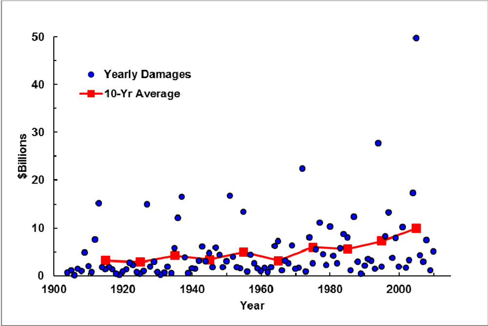
3. Floods in Iowa
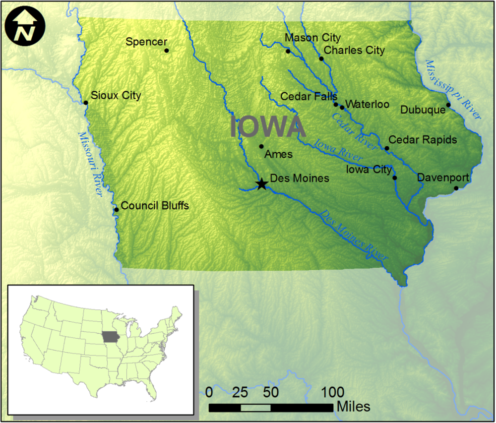
3.1. Study Area

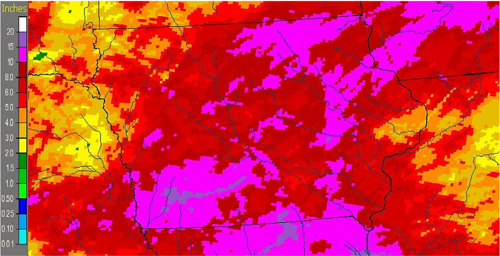
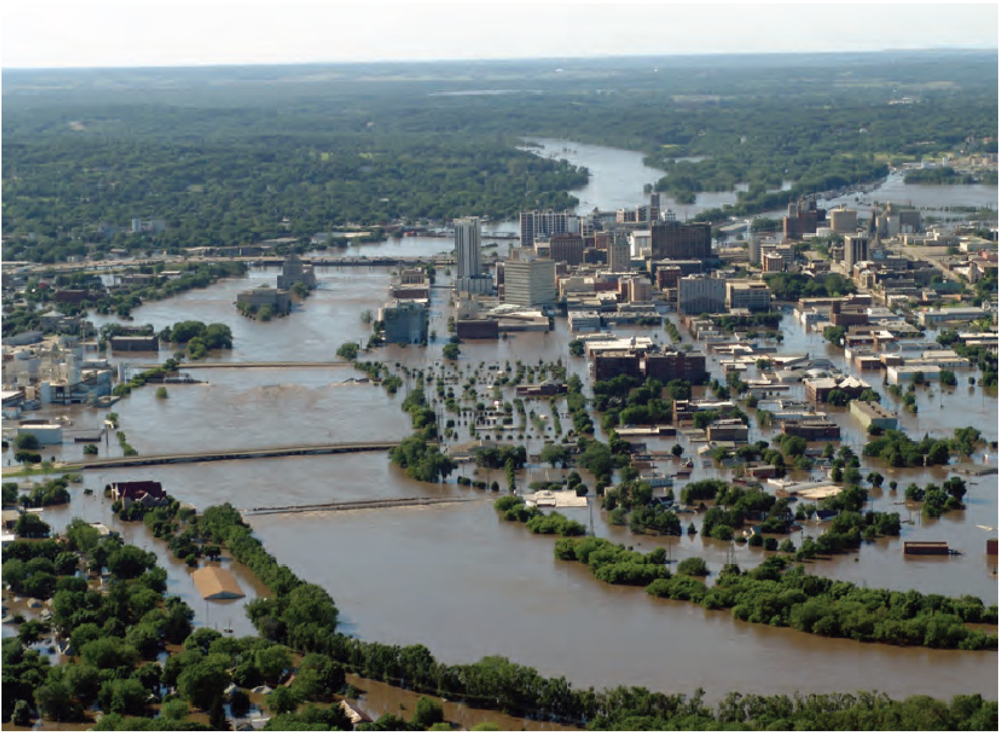
3.2. Historic Floods
3.3. Establishment of the Iowa Flood Center
4. Statewide Floodplain Delineation
4.1. Introduction
4.2. Data Sources
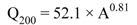
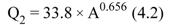
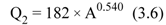
4.3. Hydrologic Analyses

| Site Description | Gage Record (Years) | Drainage Area (Square Miles) | Method | Reference |
|---|---|---|---|---|
| ungaged site on an ungaged stream | --- | 1–20 | 1987 methods for return intervals ≤ 100 years, extrapolated 1987 equations > 100 years | Lara 1987 [35], Appendix |
| --- | 20–50 | average the 1987 or extrapolated 1987 equations and 2001 methods | Lara 1987 [35], Eash 2001 [28], Appendix | |
| --- | >50 | 2001 single-parameter regression equations | Eash 2001 [28] | |
| gaged site | --- | --- | weighted estimates for gaged sites | Eash 2001 [28] |
| ungaged site on a gaged stream | <25 | --- | regression-weighted estimate for ungaged sites | Eash 2001 [28] |
| ≥25 | --- | area-weighted estimate for ungaged sites | Eash 2001 [28] |
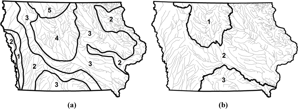
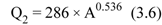
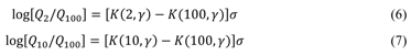
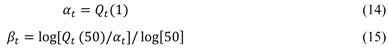
4.3.1. Drainage Areas Between 1 and 20 Square Miles
| Region 1 | Region 2 | Region 3 | Region 4 | Region 5 |
|---|---|---|---|---|
 |  |  |  |  |
 |  |  |  |  |
 |  |  |  |  |
 |  |  |  |  |
 |  |  |  |  |
 |  |  |  |  |

| Region 1 | Region 2 | Region 3 | Region 4 | Region 5 |
|---|---|---|---|---|
 |  |  |  |  |
 |  |  |  |  |
4.3.2. Drainage Areas Between 20 and 50 Square Miles
| Region 1 | Region 2 | Region 3 |
|---|---|---|
 |  |  |
 |  |  |
 |  |  |
 |  |  |
 |  |  |
 |  |  |
 |  |  |
 |  |  |
4.3.3. Drainage Areas Greater than 50 Square Miles
4.3.4. Gaged Locations

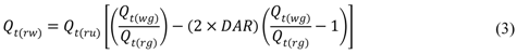
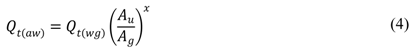
4.3.5. Ungaged Locations on Gaged Streams

4.4. Hydraulic Modeling
4.4.1 Overview
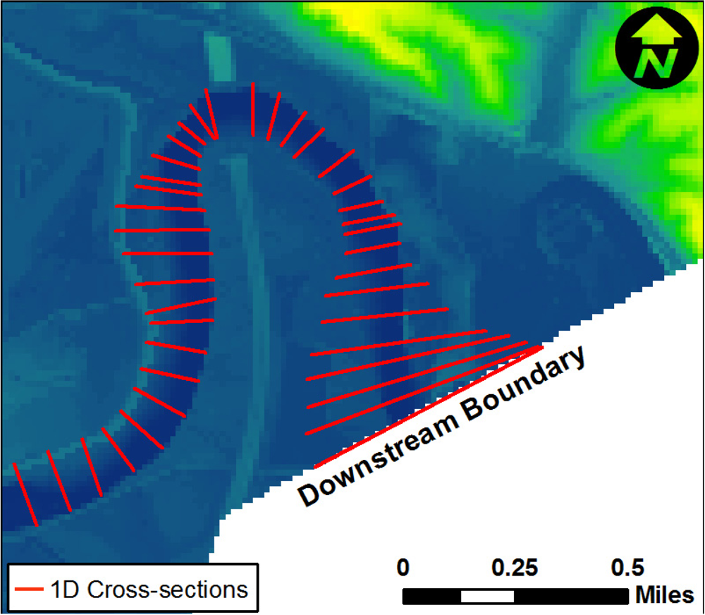
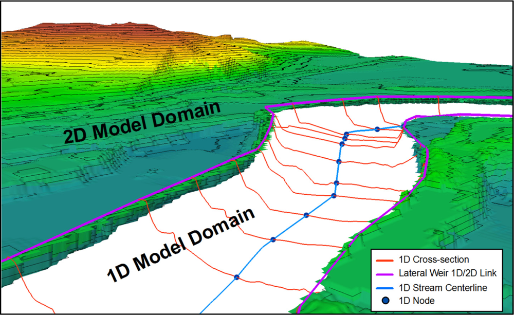
4.4.2. Model Development
4.4.3. Boundary Conditions
4.4.4. Mapping of Simulation Results
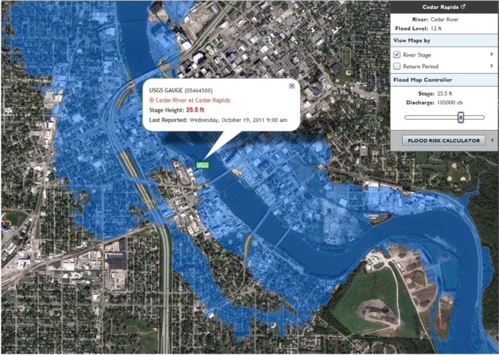
4.5. Public Availability and Implementation
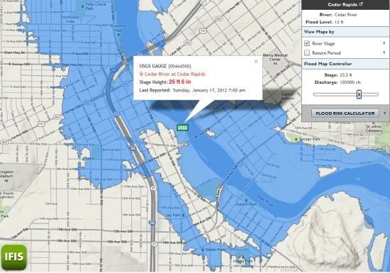
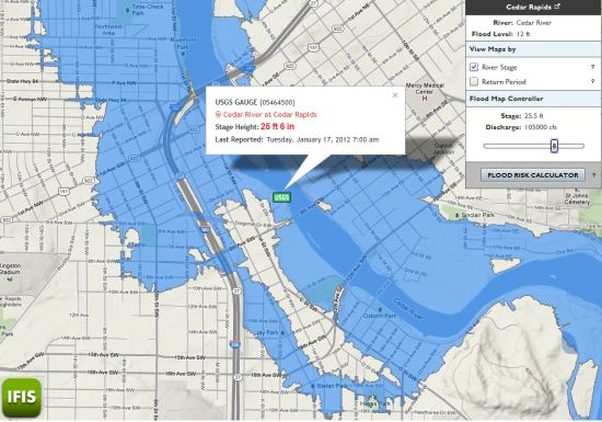
5. Detailed Urban Flood Mapping
5.1. Introduction
5.2. Data Sources
5.3. Hydraulic Modeling
5.3.1. Overview
5.3.2. Model Development
5.3.3. Boundary Conditions

5.3.4. Model Calibration
5.3.5. Development of Inundation Map Libraries
5.4. Public Availability

6. Summary and Discussion
Acknowledgments
References
- NWS. Flood Losses: Compilation of Flood Loss Statistics; National Weather Service: Fort Worth, TX, USA, 2010. Available online: http:nws.noaa.gov/oh/hic/flood_stats/flood_loss_time_series.shtml (accessed on 1 September 2011).
- Pielke, R.A., Jr.; Downton, M.W.; Miller, J.Z.B. Flood Damage in the United States,1926–2000: A Reanalysis of National Weather Service Estimates; National Center for Atmoshperic Research: Boulder, CO, USA, 2002. [Google Scholar]
- Downton, M.W.; Miller, J.Z.; Pielke, R.A., Jr. Reanalysis of U.S. National Weather Service flood loss database. Nat. Hazards Rev. 2005, 6, 13–22. [Google Scholar] [CrossRef]
- Lott, N.; Ross, T. Tracking Billion-Dollar U.S. Weather Disasters; American Meteorological Society: Boston, MA, USA, 2006; volume 87, pp. 557–559. [Google Scholar]
- Trenberth, K.E.; Jones, P.D.; Ambenje, P.; Bojariu, R.; Easterling, A.; Klein Tank, A.; Parker, D.; Rahimzadeh, F.; Renwick, J.A.; Rusticucci, M.; et al. Observations: Surface and atmospheric climate change. In Climate Change 2007: The Physical Science Basis. Contribution of Working Group I to the Fourth Assessment Report of the Intergovernmental Panel on Climate Change; Solomon, S., Qin, D., Manning, M., Chen, Z., Marquis, M., Averyt, K.B., Tignor, M., Miller, H.L., Eds.; Cambridge University Press: Cambridge, UK and New York, NY, USA, 2007. [Google Scholar]
- Milly, P.C.D.; Dunne, K.A.; Vecchia, A.V. Global pattern of trends in streamflow and water availability in a changing climate. Nature 2005, 438, 347–350. [Google Scholar]
- Milly, P.C.D.; Wetherald, R.T.; Dunne, K.A.; Delworth, T.L. Increasing risk of great floods in a changing climate. Nature 2002, 415, 514–517. [Google Scholar]
- Burby, R.J. Flood insurance and floodplain management: The US experience. Glob. Environ. Change Part B 2001, 3, 111–122. [Google Scholar]
- Fridirici, R. Floods of people: New residential development into flood-prone areas in San Joaquin County, California. Nat. Hazards Rev. 2008, 9, 158–168. [Google Scholar]
- Burningham, K.; Fielding, J.; Thrush, D. It’ll never happen to me? Understanding public awareness of local flood risk. Disasters 2008, 32, 216–238. [Google Scholar]
- Baan, P.J.; Klijn, F. Flood risk perception and implications for flood risk management. Int. J. River Basin Manag. 2004, 2, 133–122. [Google Scholar]
- Stefanovic, I.L. The contribution of philosophy to hazards assessment and decision making. Nat. Hazards 2003, 28, 229–247. [Google Scholar] [CrossRef]
- Mileti, D.S. Disasters by Design: A Reassessment of Natural Hazards in the United States; Joseph Henry Press: Washington, DC, USA, 1999. [Google Scholar]
- FEMA, National Flood Insurance Program: Program Description; Federal Emergency Management Agency: Government Printing Office, Washington, DC, USA, 2002.
- NFIP. Claim Information; National Flood Insurance Program: Washington, DC, USA, 2011. Available online: http://bsa.nfipstat.com/reports/1011.htm (accessed on 1 September 2011).
- Anderson, D.R. The national flood insurance program—Problems and potential. J. Risk Insur. 1974, 41, 579–599. [Google Scholar]
- Bell, H.M.; Tobin, G.A. Efficient and effective? The 100-year flood in the communication and perception of flood risk. Environ. Hazards 2007, 7, 302–311. [Google Scholar]
- ASFPM, National Flood Programs in Review—2000; Association of State Floodplain Managers: Madison, WI, USA, 2000.
- Sarewitz, D.; Pielke, R., Jr.; Keykhah, M. Vulnerability and risk: Some thoughts from a political and policy perspective. Risk Anal. 2003, 23, 805–810. [Google Scholar]
- GAO, Flood Map Modernization: Program Strategy Shows Promise, but Challenges Remain; United States General Accounting Office, Government Printing Office: Washington, DC, USA, 2004.
- NRC, Mapping the Zone: Improving Flood Map Accuracy; National Research Council of the National Academies, The National Academies Press: Washington, DC, USA, 2009.
- NRC, Elevation Data for Floodplain Mapping; National Research Council of the National Academies, The National Academies Press: Washington, DC, USA, 2007.
- NCFMP, North Carolina Floodplain Mapping Program: 2000–2008 Program Review; North Carolina Floodplain Mapping Program, State of North Carolina: Raleigh, NC, USA, 2008.
- USGS. USGS Water Data for North Carolina; U.S. Geological Society: Reston, VA, USA, 2011. Available online: http://waterdata.usgs.gov/nc/nwis (accessed on 1 September 2011).
- Jackson, L.; Keeney, D. Perennial farming systems that resist flooding. In A Watershed Year: Anatomy of the Iowa Floods of 2008; Mutel, C.F., Ed.; University of Iowa Press: Iowa City, IA, USA, 2010. [Google Scholar]
- Wehmeyer, L.L.; Weirich, F.H.; Cuffney, T.F. Effect of land cover change on runoff curve number estimation in Iowa, 1832-2001. Ecohydrology 2011, 4, 315–321. [Google Scholar]
- Bradley, A.A., Jr. What causes floods in Iowa. In A Watershed Year: Anatomy of the Iowa Floods of 2008; Mutel, C.F., Ed.; University of Iowa Press: Iowa City, IA, USA, 2010. [Google Scholar]
- Eash, D.A. Techniques for Estimating Flood-Frequency Discharges for Streams in Iowa; Water-Resources Investigations Report 00-4233. US Geological Survey: Iowa City, IA, USA, 2001. [Google Scholar]
- Galloway, G.E. Sharing the Challenge: Floodplain Management into the 21st Century; Interagency Floodplain Management Review Committee: Washington, DC, USA, 1994. [Google Scholar]
- Linhart, S.M.; Eash, D.A. Floods of May 30 to June 15, 2008, in the Iowa River and Cedar River Basins, Eastern Iowa; U.S. Geological Survey Open-File Report. U.S. Geological Survey: Reston, VA, USA, 2010. Available online: http://pubs.usgs.gov/of/2010/1190/pdf/of2010-1190.pdf (accessed on 1 September 2011).
- Buchmiller, R.C.; Eash, D.A. Floods of May and June 2008 in Iowa; U.S. Geological Survey Open-File Report. U.S. Geological Survey: Reston, VA, USA, 2010. Available online: http://pubs.usgs.gov/of/2010/1096/pdf/OFR2010–1096.pdf (accessed on 1 September 2011).
- RIO. Rebuild Iowa Office: Quarterly Report & Economic Recovery Strategy. Rebuild Iowa Office: Des Moines, IA, USA, April 2011. Available online: http://publications.iowa.gov/11071/1/2011-04_Quarterly_Report_FINAL.pdf (accessed on 1 September 2011).
- NWS. Advanced Hydrologic Prediction Service: Monthly Observed Precipitation. National Weather Service: Silver Spring, MD, USA, 2010. Available online: http://water.weather.gov/precip/ (accessed on 1 September 2011).
- USGS. National Land Cover Database (NLCD 2001); U.S. Geological Survey: Reston, VA, USA, 2009. Available online: http://landcover.usgs.gov/uslandcover.php (accessed on 1 Septmber 2011).
- Lara, O.G. Method for Estimating the Magnitude and Frequency of Floods at Ungaged Sites on Unregulated Rural Streams in Iowa; Water-Resources Investigation Report 87-4132. U.S. Geological Survey: Iowa City, IA, USA, 1987. [Google Scholar]
- Iowa Department of Transportation. LRFD Design Manual; Iowa Department of Transportation: Ames, IA, USA, 2010. Available online: http://www.iowadot.gov/bridge/manuallrfd.htm (accessed on 1 September 2011).
- Bradley, A.A., Jr. Extrapolation of Flood Frequency Regression Curves; IIHR—Hydroscience and Engineering: Iowa City, IA, USA, 2011. [Google Scholar]
- Eash, D.A. Estimating Design-Flood Discharges for Streams in Iowa Using Drainage-Basin and Channel-Geometry Characteristics; Water-Resources Investigation Report 93-4062. U.S. Geological Survey: Iowa City, IA, USA, 1993. [Google Scholar]
- Hydrology Subcommittee of the Interagency Advisory Committee on Water Data. In Guidelines for Determining Flood Flow Frequency. Bulletin 17B of the Hydrology Subcommittee; Office of Water Data Coordination, U.S. Geological Survey: Reston, VA, USA, 1982.
- Chow, V.T. Open-Channel Hydraulics; McGraw-Hill: New York, NY, USA, 1959. [Google Scholar]
- FEMA, Guidelines and Specification for Flood Hazard Mapping Partners: Appendix C: Guidance for Riverine Flooding Analyses and Mapping; Federal Emergency Management Agency, Government Printing Office: Washington, DC, USA, 2002.
- IFC. Maps; The Iowa Flood Center: Iowa City, USA, 2009. Available online: http://www.iowafloodcenter.org/maps (accessed on 1 September 2011).
- Gall, M.; Boruff, B.J.; Cutter, S.L. Assessing flood hazard zones in the absence of digital floodplain maps: Comparison of alternative approaches. Nat. Hazards Rev. 2007, 8, 1–12. [Google Scholar]
- Bates, P.D.; de Roo, A.P.J. A simple raster-based model for flood inundation simulation. J.ournal Hydrol. 2000, 236, 54–77. [Google Scholar]
- Tayefi, V.; Lane, S.N.; Hardy, R.J.; Yu, D. A comparison of one- and two-dimensional approaches to modelling flood inundation over complex upland floodplains. Hydrol. Process. 2007, 21, 3190–3202. [Google Scholar]
- McMillan, H.K.; Brasington, J. Reduced complexity strategies for modelling urban floodplain inundation. Geomorphology 2007, 90, 226–243. [Google Scholar]
- DHI, MIKE FLOOD:1D-2D Modelling User Manual; DHI Water and Environment: Hørsholm, Denmark, 2009.
- IFC. Iowa Flood Information System; The Iowa Flood Center: Iowa City, USA, 2011. Available online: www.iowafloodcenter.org/ifis (accessed on 1 September 2011).
Appendix


Reference
- Lara, O.G. Method for Estimating the Magnitude and Frequency of Floods at Ungaged Sites on Unregulated Rural Streams in Iowa; Water-Resources Investigation Report 87-4132. U.S. Geological Survey: Iowa City, IA, USA, 1987. [Google Scholar]
- Bradley, A.A., Jr. Extrapolation of Flood Frequency Regression Curves; IIHR—Hydroscience and Engineering: Iowa City, IA, USA, 2011. [Google Scholar]
- Kite, G.W. Frequency and Risk Analyses in Hydrology; Water Resources Publications: Fort Collins, CO, USA, 1977. [Google Scholar]
© 2012 by the authors; licensee MDPI, Basel, Switzerland. This article is an open-access article distributed under the terms and conditions of the Creative Commons Attribution license (http://creativecommons.org/licenses/by/3.0/).
Share and Cite
Gilles, D.; Young, N.; Schroeder, H.; Piotrowski, J.; Chang, Y.-J. Inundation Mapping Initiatives of the Iowa Flood Center: Statewide Coverage and Detailed Urban Flooding Analysis. Water 2012, 4, 85-106. https://doi.org/10.3390/w4010085
Gilles D, Young N, Schroeder H, Piotrowski J, Chang Y-J. Inundation Mapping Initiatives of the Iowa Flood Center: Statewide Coverage and Detailed Urban Flooding Analysis. Water. 2012; 4(1):85-106. https://doi.org/10.3390/w4010085
Chicago/Turabian StyleGilles, Daniel, Nathan Young, Harvest Schroeder, Jesse Piotrowski, and Yi-Jia Chang. 2012. "Inundation Mapping Initiatives of the Iowa Flood Center: Statewide Coverage and Detailed Urban Flooding Analysis" Water 4, no. 1: 85-106. https://doi.org/10.3390/w4010085