Climate Change Impacts on Water Availability and Use in the Limpopo River Basin

Abstract

This paper analyzes the effects of climate change on water availability and use in the Limpopo River Basin of Southern Africa, using a linked modeling system consisting of a semi-distributed global hydrological model and the Water Simulation Module (WSM) of the International Model for Policy Analysis of Agricultural Commodities and Trade (IMPACT). Although the WSM simulates all major water use sectors, the focus of this study is to evaluate the implications of climate change on irrigation water supply in the catchments of the Limpopo River Basin within the four riparian countries: Botswana, Mozambique, South Africa, and Zimbabwe. The analysis found that water resources of the Limpopo River Basin are already stressed under today’s climate conditions. Projected water infrastructure and management interventions are expected to improve the situation by 2050 if current climate conditions continue into the future. However, under the climate change scenarios studied here, water supply availability is expected to worsen considerably by 2050. Assessing hydrological impacts of climate change is crucial given that expansion of irrigated areas has been postulated as a key adaptation strategy for Sub-Saharan Africa. Such expansion will need to take into account future changes in water availability in African river basins.

1. Introduction

Increasing evidence suggests that anthropogenic climate change is already underway [1]. Climate change affects hydrological cycles locally [2] and globally [3]. It alters the amount and timing of river flow, challenges the coping capacities of existing water infrastructure and management systems, and brings higher risks of water shortages and floods. Meanwhile, the implications of climate change can go well beyond the water sector since many of the most serious effects of climate change on non-water areas are mediated via water [4]. For instance, the Intergovernmental Panel on Climate Change (IPCC) identifies food systems as a key area vulnerable to climate change, along with water and three other sectors [5]. In general, the water and agricultural sectors experience the most direct impacts from climate change due to their direct exposure to and dependence on weather and other natural conditions.

Semi-arid and arid areas are particularly exposed to the adverse impacts of climate change on freshwater [6]. Many such areas have developed extensive irrigation systems, such as the western United States, Northern China, semi-arid areas in India and Pakistan, and the majority of the Mediterranean basin, in order to meet crop water requirements that cannot be satisfied by precipitation alone, particularly during the dry season or in drought years. However, there are other semi-arid and arid areas with relatively low level of irrigation development for socioeconomic reasons or lack of reliable water resources. Farming in these areas is no doubt difficult and risky, and the dry and volatile climate is often a cause of underdevelopment and persistent poverty [7]. Assessing climate change impacts on such areas is particularly important in order to act proactively to minimize adverse impacts and to plan appropriately for the long-term well-being of the rural population living in these areas. The Limpopo River Basin (LRB) in Southern Africa is such an area and this paper analyzes climate change impacts on water availability and use in the basin.

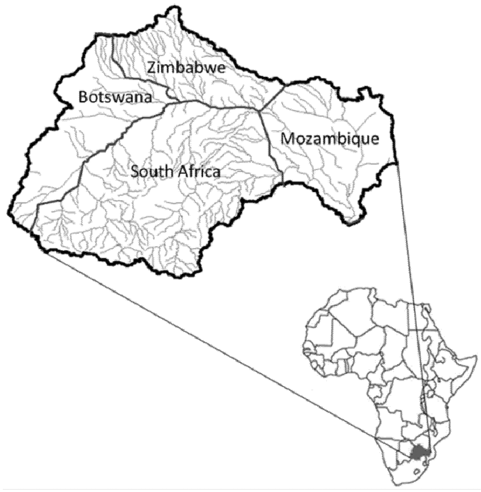
The LRB covers an area of more than 412 thousand km². It spreads over four countries: Botswana, Mozambique, South Africa, and Zimbabwe; its main-stem is the international boundary between South Africa and Botswana, and South Africa and Zimbabwe (Figure 1). The river originates from the highlands that separate South Africa from Botswana and Zimbabwe, and flows through and between these countries before it enters Mozambique and finally drains into the Indian Ocean [8]. As shown in Table 1, by area, 45 percent of the basin is in South Africa, 19 percent in Botswana, 21 percent in Mozambique, and 15 percent in Zimbabwe [8,9].

The climate in the LRB ranges from tropical rainy along the coastal plain of Mozambique to tropical dry savannah and tropical dry desert further inland, south of Zimbabwe. Annual precipitation varies between 250 millimeters (mm) in the hot, dry western and central areas to 1,050 mm in the high-rainfall eastern escarpment areas. Precipitation is highly seasonal and unevenly distributed spatially, with about 95 percent of precipitation occurring between October and April [8]. Precipitation also varies significantly from year to year [10]. These precipitation characteristics limit crop production because annual precipitation mainly occurs during a short summer rain season with high inter-annual variations. Flooding and droughts are major water-mediated impacts of climate change in the LRB [9]. Table 1 also shows annual mean precipitation and potential evapotranspiration for each of the four country catchments of the basin.

Figure 1. Map of the Limpopo River Basin and boundaries of the four riparian countries. Source: Adapted from IDIS Basin Kit database [11].

Figure 1. Map of the Limpopo River Basin and boundaries of the four riparian countries. Source: Adapted from IDIS Basin Kit database [11].

Table 1. Characteristics of the Limpopo River Basin catchments in riparian countries.

Country	Area of country within basin (km2)	Share of total basin area (%)	Annual mean precipitation (mm)	Annual mean potential evapotranspiration (mm)
Botswana	80118	19	422	1599
Mozambique	84981	21	751	1650
South Africa	185298	45	607	1570
Zimbabwe	62541	15	506	1592
Basin	412938	100	587	1596

Sources: (1) Area of country in basin [8]; (2) Share of total basin area [8]; (3) Annual mean precipitation: authors’ calculation based on the 1971–2000 monthly precipitation data from the CRU TS 2.1 climatology [12]; (4) Annual mean potential evapotranspiration: authors’ calculation using Priestley-Taylor equation based on the 1971–2000 monthly data series from the CRU TS 2.1 climatology [12].

Table 1. Characteristics of the Limpopo River Basin catchments in riparian countries.

Country	Area of country within basin (km2)	Share of total basin area (%)	Annual mean precipitation (mm)	Annual mean potential evapotranspiration (mm)
Botswana	80118	19	422	1599
Mozambique	84981	21	751	1650
South Africa	185298	45	607	1570
Zimbabwe	62541	15	506	1592
Basin	412938	100	587	1596

Sources: (1) Area of country in basin [8]; (2) Share of total basin area [8]; (3) Annual mean precipitation: authors’ calculation based on the 1971–2000 monthly precipitation data from the CRU TS 2.1 climatology [12]; (4) Annual mean potential evapotranspiration: authors’ calculation using Priestley-Taylor equation based on the 1971–2000 monthly data series from the CRU TS 2.1 climatology [12].

The LRB has a population of approximately 14 million, evenly divided between rural (52 percent) and urban (48 percent) areas [9]. The total harvested crop area is 2.9 million hectares, and 91 percent of the area is cropped under rain-fed conditions [9].

With generally lagging water infrastructure development and rapidly increasing populations, water use in the Limpopo River Basin is expected to face serious water scarcity. Water scarcity has thus become a limiting factor for economic development in the basin, as it has in many other basins located in developing countries with arid climates, lagging water infrastructure development, and rapidly increasing populations [9].

Climate change impacts in the LRB have not been studied in-depth. Existing studies analyzed inter-annual variability of dry and wet spells over the basin [10], explored the rainfall-runoff relationships at sub-basins, and looked into the consequences of extreme events such as droughts [8]. However, climate change impacts on water resources have not yet been assessed at the basin level to the best knowledge of the authors, and key questions remain unaddressed in this regard. In this paper, we try to fill this gap by evaluating climate change impacts on water availability and use in the basin, using multiple climate change scenarios and taking into account plausible socioeconomic developments.

2. Linked Modeling System for Water Availability and Use Simulation

Assessing climate change impacts in the water sector requires analytic models to quantitatively evaluate water availability and allocation under both present and changed climate conditions. For this purpose, we use a linked modeling system adapted to the particular condition of the LRB. The linked modeling system consists of a semi-distributed Global Hydrological Model (GHM) [13] and the Water Simulation Module (WSM) of the International Model for Policy Analysis of Agricultural Commodities and Trade (IMPACT) developed at the International Food Policy Research Institute (IFPRI) [14,15]. Both the GHM and the WSM cover global river basins including the LRB. This paper utilizes the LRB component of the GHM and the WSM to analyze the impacts of climate change on water availability and use. Although the WSM simulates all major water use sectors, the focus of this study is to evaluate the implications of climate change on irrigation water supply in the Limpopo catchments in the four riparian countries: Botswana, Mozambique, South Africa, and Zimbabwe.

Figure 2. Structures of and linkage between the semi-distributed hydrological model and the water simulation module of the International Model for Policy Analysis of Agricultural Commodities and Trade (IMPACT).

Figure 2. Structures of and linkage between the semi-distributed hydrological model and the water simulation module of the International Model for Policy Analysis of Agricultural Commodities and Trade (IMPACT).

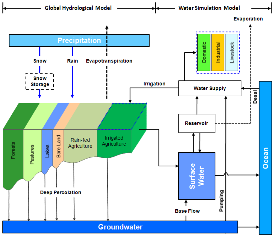
Figure 2 illustrates the structures of the linked modeling system. In a river basin, the GHM hydrological model simulates the rainfall-runoff process, taking into account land cover classes in computing the potential evapotranspiration. The WSM water management model simulates reservoir regulation of natural flow and abstraction of groundwater, according to the estimated total water demand consisting of domestic, industrial, livestock and irrigation sectors. The WSM uses the monthly total runoff and potential evapotranspiration calculated by the GHM to simulate water management and allocation. On the top of Figure 2, the double headed arrows define the functional domains of the GHM and the WSM. In the next sections we describe the two models in more detail.

2.1. Hydrological Model

The GHM hydrological model is a semi-distributed parsimonious model. It simulates monthly soil moisture balance, evapotranspiration and runoff generation on each 0.5° latitude by 0.5° longitude grid cell spanning over the global land surface except for the Antarctic. The model uses gridded monthly precipitation, temperature, vapor pressure and cloud cover data from the CRU TS 2.1 database [12] as climate forcing. Gridded output of hydrological fluxes, namely effective rainfall (for calculating net irrigation water requirement in the WSM), potential/actual evapotranspiration and runoff, are spatially aggregated to Food Production Units (FPU) [13,15] within the river basin. They are weighted by grid cell areas, and then incorporated into the WSM. FPUs are determined by country and river basin boundaries. The LRB consists of four FPUs, one in each riparian country.

The most dominant climatic drivers for water availability are precipitation and evaporative demand determined by net radiation at ground level, atmospheric humidity, wind speed and temperature. In the GHM hydrological model, the Priestley-Taylor Equation [16] is used to calculate potential evapotranspiration:

   (1)

In Equation (1), PET is the potential evapotranspiration in mm per day; the value of α is 1.26 for a humid climate and 1.74 in arid locations. The humid and arid conditions are defined respectively as having relative humidity above or below 60 percent in the month with peak evapotranspiration [17]; Δ is the slope of the vapor pressure curve in kPa·°C⁻¹; γ is the psychrometric constant in kPa·°C⁻¹; R_n is the net radiation at the land surface in mm per day; and G is the soil heat flux density in mm per day.

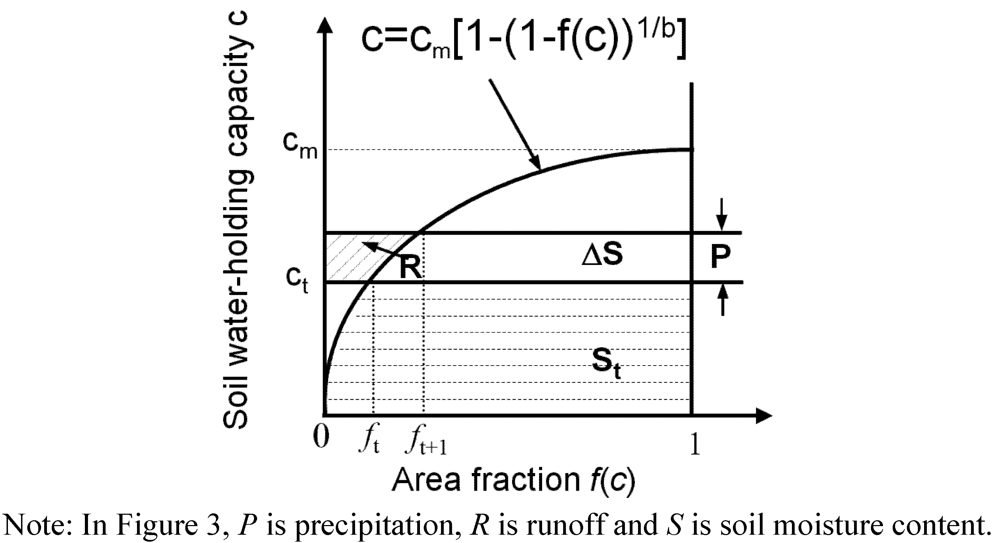
Soil moisture balance is simulated at each grid cell using a single layer water bucket. To represent subgrid variability of soil water-holding capacity c, we assume that it varies spatially within each grid cell, following a parabolic distribution function [18,19,20].

   (2)

where is the fraction of area in a grid cell that has soil water-holding capacity values lower than c; C_m is the maximum soil water-holding capacity value across all points within the grid cell; and b is the “shape parameter” that defines the degree of spatial variability of soil moisture holding capacity c.

The maximum amount of water that can be held in the grid cell is

   (3)

In Figure 3, S_m equals the area between the parabolic curve and the x axis, with area fraction values of the x axis ranging from zero to one.

Figure 3. Distribution of soil water-holding capacity in a 0.5° latitude × 0.5° longitude grid cell.

Figure 3. Distribution of soil water-holding capacity in a 0.5° latitude × 0.5° longitude grid cell.

Assuming that, at any time t, each point in the grid cell is either at C_m or at a constant moisture state c [17], the mean areal water storage S associated with soil water- holding capacity c at time t is

   (4)

With precipitation P_t and actual evapotranspiration AET_t in time period t, runoff is determined by the following equations [18,19]:

If ,

   (5)

Otherwise, if ,

   (6)

The AET is determined jointly by the PET and the relative soil moisture state in a grid cell at time period t:

   (7)

Runoff generated in time period t is divided into a surface runoff component RS and a deep percolation component using a partitioning factor :

   (8)

A linear reservoir is assumed to model base flow RB. The storage of the linear reservoir is linearly related to output, namely base flow, by a storage constant β [21]:

   (9)

where G_t is the storage value in time period t. The change of reservoir storage during time period t equals the difference between deep percolation and base flow which occurred in this period:

   (10)

Total runoff generated in time period t is the sum of surface runoff and base flow:

   (11)

In the above equations, calibration parameters include the sub-grid variability shape parameter b, the total runoff partitioning parameter λ, the storage constant β, and the average soil water holding capacity S_m. Conceptually, S_m should be equal to available water, namely field capacity less wilting point, in a soil moisture accounting perspective. However, because of the monthly time step adopted, using measured available water rather than calibrating S_m can significantly overestimate runoff and underestimate actual evapotranspiration as found out in our calibration experiments.

A lack of adequately long and continuous streamflow records in the LRB made hydrological model calibration using such records not possible. In this study, the simulated gridded monthly runoff series of the WaterGAP Global Hydrological Model [22,23] were used to calibrate the parameters for grid cells in the Limpopo River Basin. We use a genetic algorithm [24] to minimize the mean square error between the simulated runoff and “observed” runoff time series.

Figure 4. Runoff calibration and validation for the Limpopo River Basin.

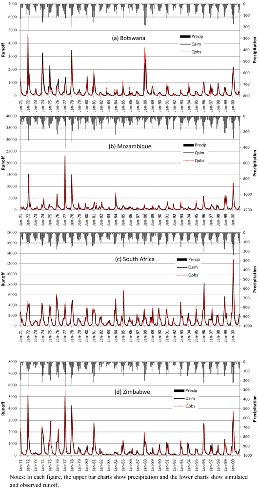
Figure 4. Runoff calibration and validation for the Limpopo River Basin.

Figure 4 shows precipitation, simulated and observed runoff for the calibration period 1971–85 and the validation period 1986–2000. A visual inspection of the simulated and observed flow series in Figure 4 suggests that the GHM can simulate monthly runoff reasonably well, and model performance in the validation period is nearly as good as that in the calibration period. We also use the Nash-Sutcliffe model efficiency coefficient (NSE) [25] to quantitatively evaluate model performance, which is given as

   (12)

In Equation (12), represents the observed flow in time period t, denotes the average of the observed flow over the entire simulation period, and is the simulated flow for time period t. By definition, the NSE value ranges from −∞ to 1, and the closer the model efficiency is to 1, the more accurate the model is. In our simulations for the Limpopo catchments, the NSE values are 0.913 and 0.906 in the calibration period and validation period, respectively, for the catchment in Botswana, 0.976 and 0.947 in Mozambique, 0.980 and 0.985 in South Africa, and 0.964 and 0.962 in Zimbabwe.

2.2. Water Simulation Module

The WSM of IMPACT simulates water demand, supply, reservoir storage regulation, and surface and ground water withdrawals at monthly time periods, using FPU, usually a basin or sub-basin, as the fundamental unit of depletion accounting [15]. Using the lumped unit avoids tracking detailed water use processes as occurs with conventional river basin management models. When the scale of analysis goes from basin down to the irrigation system level and then to the field scale, water flow pathways become increasingly complex and consequently water balance calculations for depletion accounting quickly become non-tractable unless the geographic domain of analysis is compromised. In addition, sophisticated water accounting relies on extensive flow measurements, which is almost impossible for a global water model like the WSM.

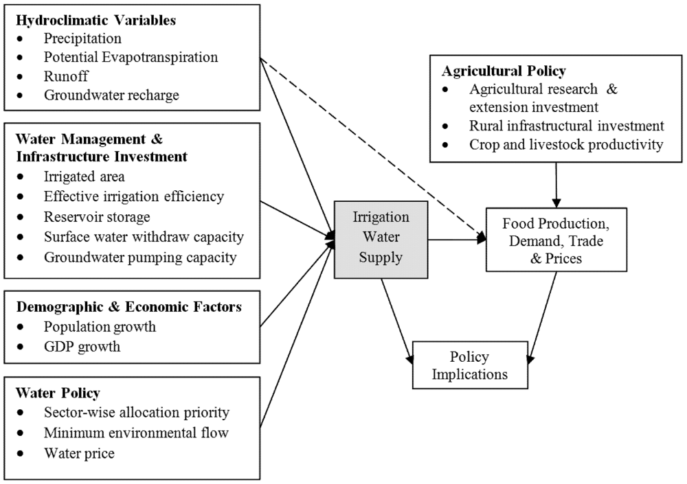
The WSM optimizes water supply based on water demands, driven by several kinds of factors, as shown in Figure 5. Among these, the hydroclimatic factors include long-term monthly precipitation, potential evapotranspiration, and internal renewable water resources; the demographic and economic factors are population and Gross Domestic Product (GDP) growth rates that drive the growth of domestic and industrial water demand; water management and infrastructure investments include projected irrigated area growth, the changing rate of effective irrigation efficiency [26] at the FPU level, reservoir storage increase, changes in surface and ground water withdrawal capacities; and policy and institutional parameters such as water allocation priorities.

In optimizing water supply, the WSM firstly calculates total water supply for all sectors in each month, and then allocates the total supply to sectors in a priority-based manner. It gives first priority to domestic water demand, second priority to industrial and livestock water demand, and allocates the remaining water supply to irrigation. It is worth noting that minimum environmental flow is considered as a constraint in water supply optimization, thus environmental flow requirement is not compromised by allocating remaining water supply to irrigation. Total irrigation water supply is further allocated to crops according to crop water requirements [27]. Flow regulation by surface storage, diversion of surface water to users and groundwater pumping are constrained by their capacities that change over time according to prescribed growth rates. Minimum environmental flow requirements are treated as a hard constraint in the model.

Figure 5. Driving forces in the Water Simulation Module and its linkages with the Food Module in IMPACT.

Figure 5. Driving forces in the Water Simulation Module and its linkages with the Food Module in IMPACT.

Thus, the WSM focuses on the water that can be managed—streamflow and groundwater, also referred to as “blue water” [28]. The portion of crop-evapotranspirated water from rain or snow, namely “effective rainfall”, is considered in estimating irrigation water requirements.

The WSM simulates water balances at the FPU scale up to 2050. The four FPUs within the LRB are connected by their relative upstream–downstream relationship, with the outflow from an upstream FPU being the inflow of the immediate downstream FPU. The “water-mediated” climate change impacts are channeled to irrigation and crop production in the IMPACT model through changes taken place in the hydrological cycle, including precipitation, runoff and crop-specific potential evapotranspiration.

3. Climate Change and Socioeconomic Scenarios

3.1. Climate Change Scenarios

In the coming decades, precipitation in southern Africa will likely decrease and temperature increase will very likely surpass global annual mean warming [29]. To evaluate the water resource impacts of a potentially drier and warmer climate, we use climate projections produced by General Circulation Models (GCM), the simulation tools that account for the complex set of climate-related processes occurring in the coupled atmosphere-land surface-ocean-sea ice system. Considerations of the facts associated with GCMs and emissions, guided our climate change scenario design. Firstly, GCM projections are currently subject to significant uncertainties in the modeling process. As a result, for the same emissions scenario, different GCMs produce different geographical patterns of change, particularly with respect to precipitation, the most important driver for freshwater resources [6]. Secondly, climate model uncertainties generally play a more important role between now and about 2050 than emission scenarios because greenhouse gas concentration scenarios diverge substantially only after that and because changes before 2050 include a substantially delayed response to previous emissions [30]. With these considerations, we limit our analysis, which focuses on 2050, to one emissions scenario, the medium-emission scenario SRES A1b [31], but use more than one GCM.

Our climate change scenarios for the LRB are based on the work of Jones et al. [32], who statistically downscaled a number of GCM projections, based on data available from the World Climate Research Program’s (WCRP’s) Coupled Model Intercomparison Project Phase 3 (CMIP3) multi-model dataset [32]. We evaluated precipitation changes in the downscaled GCM projections under the A1b SRES scenario, and selected projections by the CNRM-CM3 and ECHam5 GCMs, which project “moderate” and “serious” precipitation declines under climate change in the LRB, respectively.

In climate change scenario construction, we calculated the gridded mean monthly changes of precipitation and temperature between a historical period and a future period centered at 2050 from the downscaled climate dataset of Jones et al. [32], for each 0.5° × 0.5° grid cell within the LRB, and then imposed these monthly mean changes on the historical monthly gridded precipitation and temperature series of 1970–2000 from the CRU TS 2.1 global climate database [12]. The 1970–2000 series CRU data is regarded as baseline climate. For precipitation, the relative changes are applied as multipliers to adjust the 1970–2000 precipitation series; for temperature, derived absolute mean monthly changes are directly added onto the 1970–2000 temperature series. The baseline climate and the constructed climate change scenarios are used in the GHM hydrological model to simulate evapotranspiration and water availability. For convenience, we hereafter call the baseline “NoCC”, and call the two GCM-based scenarios “CNRM” and “ECHAM” respectively.

3.2. Socioeconomic Scenario

In the WSM, water demands in the domestic and industrial sectors are directly driven by per capita GDP, which is determined by the growth rates of population and GDP [14,15]. We use the medium variant population projections of the United Nations completed in 2008 and country-level GDP growth rates developed by IFPRI and the World Bank, with updates for Sub-Saharan Africa and South Asian countries. These projections were discussed in detail in Nelson et al. [33].

3.3. Irrigation and Water Infrastructure Development Scenarios

The LRB has little arable land and very low agricultural potential due to its semi-arid climate, leaving the eight million rural people in the basin with special challenges to make a living [8]. Irrigation development can significantly raise agricultural productivity by enabling crop production in dry years and during the dry season. However, the potential for irrigation development in each country within the basin is limited by arable land and the amount of water available for irrigation [34]. In highly developed regions of the basin, more land is already currently irrigated than can be supported by available water resources [9].

The WSM uses harvested, irrigated crop areas at the FPU level, which were spatially aggregated from the gridded irrigated areas generated by You et al. [35] and Portmann et al. [36], with necessary adjustments to ensure that the sum of irrigated and rainfed harvested areas for each crop match those reported in the FAOSTAT global database of FAO (Food and Agriculture Organization) [37]. The WSM incorporates annual growth in irrigated harvested areas for 2000–2050 by FPU and crop. Growth rates average 2.8 percent for Botswana, 1.6 percent for Zimbabwe, 0.68 percent for South Africa and 1.7 percent for Mozambique.

Effective irrigation efficiency is expected to increase in all Limpopo catchments over the projection period, owing to improvement in irrigation infrastructure and management. The estimated basin efficiency value in 2000 is 0.55 for the Limpopo catchment in South Africa, and 0.49 in the Limpopo catchments of the other three riparian countries. We assume that by 2050 effective irrigation efficiency will reach 0.61 in South Africa and 0.52 in the other three countries.

4. Results

4.1. Hydrological Impacts

The GHM hydrological model runs for the entire 1970–2000 period for the baseline as well as for each climate change scenario. Although the two climate change scenarios represent 2050 climate, for convenience, we still call their simulation period 1970–2000 as they were built based on climate series of this historical period. In each model run, the first year is used as the spinning-up period for establishing a reasonable initial condition of soil moisture, which is otherwise virtually unknown except if using arbitrary values. Thus, only results for 1971–2000 are available for the water demand and supply analysis in the WSM. The rest of this section summarizes findings from hydrological results.

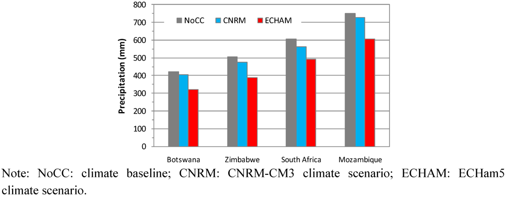
Figure 6 shows the mean annual precipitation values in the 1971–2000 climate baseline, namely the “NoCC” case, and the two climate change scenarios for 2050, in the Limpopo catchments of the four riparian countries. Geographically, precipitation declines from 750 mm in the coastal catchment in Mozambique to 600 mm in South Africa, to 500 mm in Zimbabwe and, finally to 420 mm in the further inland catchment in Botswana, under the climate baseline. Both the CNRM and the ECHAM climate change scenarios lead to lower precipitation, with ECHAM representing a stronger drop in precipitation; however the spatial gradient of precipitation does not change. Specifically, in the CNRM climate change scenario, annual mean precipitation declines by 3.8 percent in Botswana, 5.8 percent in Zimbabwe, 7.6 percent in South Africa and, 3.2 percent in Mozambique, from the climate baseline; while in the ECHAM scenario, annual mean precipitation declines by 24.2 percent in Botswana, 23.5 percent in Zimbabwe, 19.0 percent in South Africa and 19.5 percent in Mozambique.

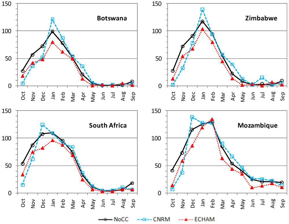
In addition to annual total changes, seasonal changes of precipitation are important for agriculture, in particular for annual crops. Analysis of monthly precipitation changes, under the two scenarios, reveals that the main precipitation reduction occurs in spring and early summer, from October through December in Botswana and Zimbabwe and from October to November in South Africa and Mozambique. Precipitation may actually increase in some months, notably in the peak precipitation months, as shown in Figure 7. However, mean annual precipitation declines in both scenarios. In Botswana, the CNRM scenario results in obvious precipitation increases from January to April and marginal increases from May to August, while precipitation declines substantially from October to December. The ECHAM scenario results in precipitation declines in all months except for a marginal increase in August, with substantial reductions taking place from October to February. In October and November, precipitation under the moderately dry CNRM scenario is lower than under the very dry ECHAM scenario. Precipitation pattern changes in Zimbabwe are largely similar to those in Botswana, under the same climate change scenarios. In South Africa and Mozambique, precipitation pattern changes are also close to those in Botswana and Zimbabwe, except that in both countries CNRM shifts the peak precipitation month from January to December.

Figure 6. Mean annual precipitation under the 1971–2000 climate baseline and climate change scenarios for 2050.

Figure 6. Mean annual precipitation under the 1971–2000 climate baseline and climate change scenarios for 2050.

Figure 7. Mean monthly precipitation (mm) under the 1971–2000 climate baseline and climate change scenarios for 2050.

Figure 7. Mean monthly precipitation (mm) under the 1971–2000 climate baseline and climate change scenarios for 2050.

Another notable feature of the precipitation patterns under climate change is that under the CNRM scenario precipitation levels in the peak month increase across all countries, although annual mean precipitation declines; even under the very dry ECHAM scenario, peak precipitation increases in Mozambique, but not in the other riparian countries. This implies a more uneven intra-annual distribution of precipitation under CNRM, with more rain concentrated in the wet months. This implies that wherever flooding is a problem in the LRB, flooding will likely worsen in the future.

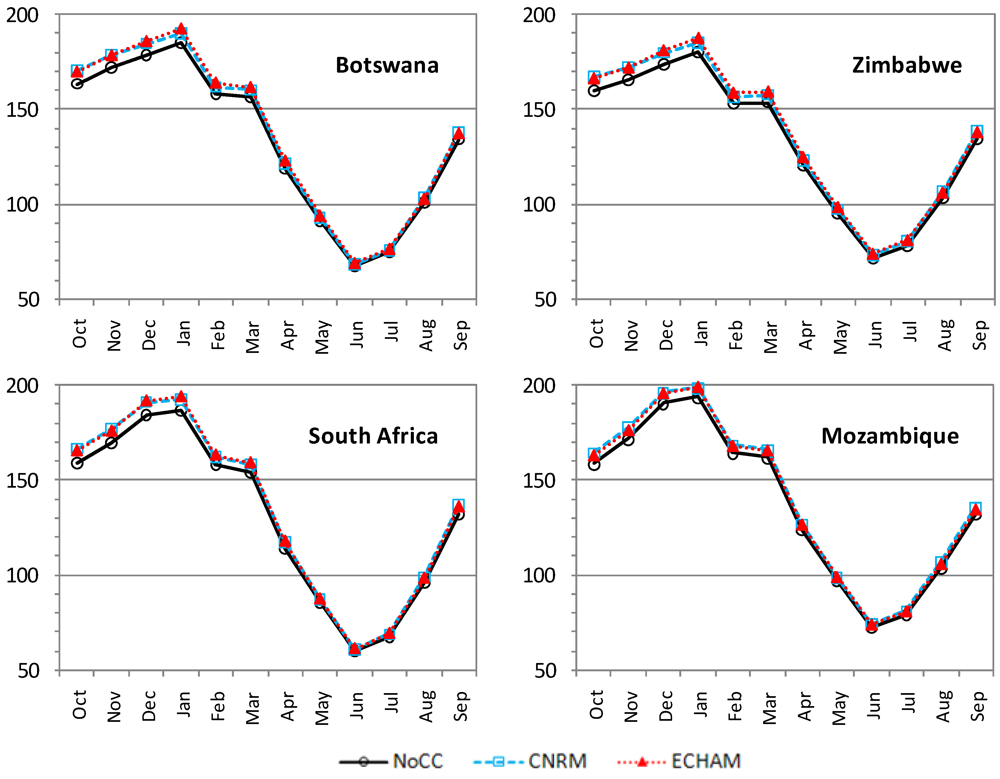
Figure 8 shows the annual mean potential evapotranspiration (PET) in the baseline and the two climate change scenarios. Spatially, PET is highest in Mozambique and lowest in South Africa. With climate change, annual mean PET increases in all riparian country catchments of the LRB; however the magnitude of the increase varies by country and by scenario. PET increases more under ECHAM than CNRM in all countries except for Mozambique. Intra-annually, PET increases more in the spring and summer seasons, and only marginally in the rest of the year, as shown in Figure 9. Overall, PET change is a less important driver of hydrological changes in the catchments, compared with changes in precipitation patterns.

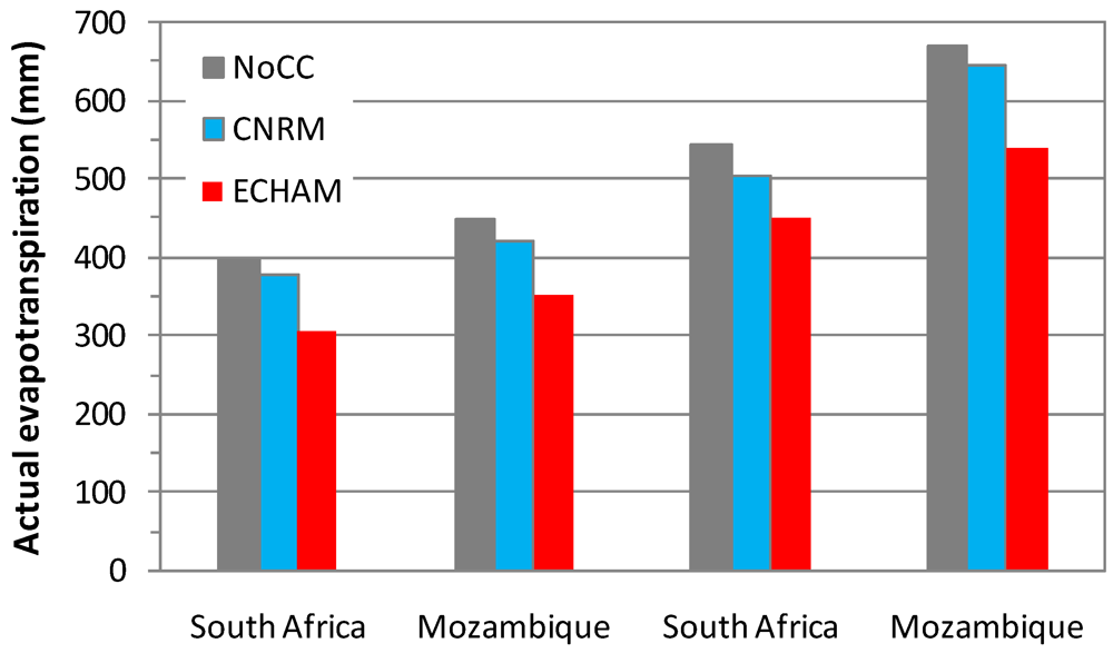
Figure 10 presents simulated mean annual actual evapotranspiration (AET) under the baseline and the two climate change scenarios. Unlike PET, which increases under climate change scenarios, AET declines under climate change, across all countries. This reflects the decline of precipitation under climate change, which replenishes soil moisture storage, the source of water that sustains evapotranspiration. Seasonally, under the CNRM scenario, AET increases in those months when precipitation increases, and major AET reductions occur in the spring and early summer months when precipitation declines significantly, as shown in Figure 11. AET under ECHAM is below baseline levels in all months.

Figure 12 displays annual mean runoff in the four riparian country catchments under baseline climate as well as under the two climate change scenarios. The ECHAM scenario causes runoff declines in all countries: 24.2 percent in Botswana, 23.5 percent in Zimbabwe, 19.0 percent in South Africa, and 19.5 percent in Mozambique. The CNRM scenario leads to more complex runoff changes. Although the annual mean precipitation declines in Botswana by 3.8 percent and in Mozambique by 3.1 percent under CNRM, simulated runoff in these two countries in fact increases by 16.6 and 0.7 percent respectively, on a yearly average.

Figure 8. Annual mean potential evapotranspiration under the 1971–2000 climate baseline and climate change scenarios for 2050.

Figure 8. Annual mean potential evapotranspiration under the 1971–2000 climate baseline and climate change scenarios for 2050.

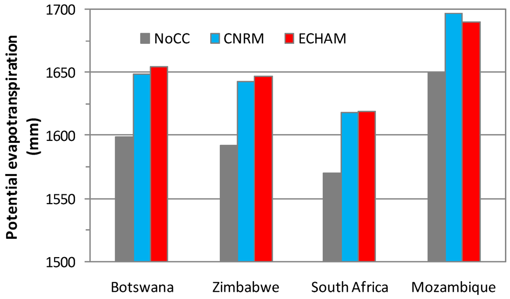
Figure 9. Mean monthly potential evapotranspiration (mm) under the 1971–2000 historical climate and climate change scenarios for 2050.

Figure 9. Mean monthly potential evapotranspiration (mm) under the 1971–2000 historical climate and climate change scenarios for 2050.

Figure 10. Simulated mean annual actual evapotranspiration under the 1971–2000 climate baseline and climate change scenarios for 2050.

Figure 10. Simulated mean annual actual evapotranspiration under the 1971–2000 climate baseline and climate change scenarios for 2050.

Figure 11. Simulated mean monthly actual evapotranspiration (mm) under the 1971–2000 climate baseline and climate change scenarios for 2050.

Figure 11. Simulated mean monthly actual evapotranspiration (mm) under the 1971–2000 climate baseline and climate change scenarios for 2050.

Figure 12. Mean annual runoff under the 1971–2000 historical climate and climate change scenarios for 2050.

Figure 12. Mean annual runoff under the 1971–2000 historical climate and climate change scenarios for 2050.

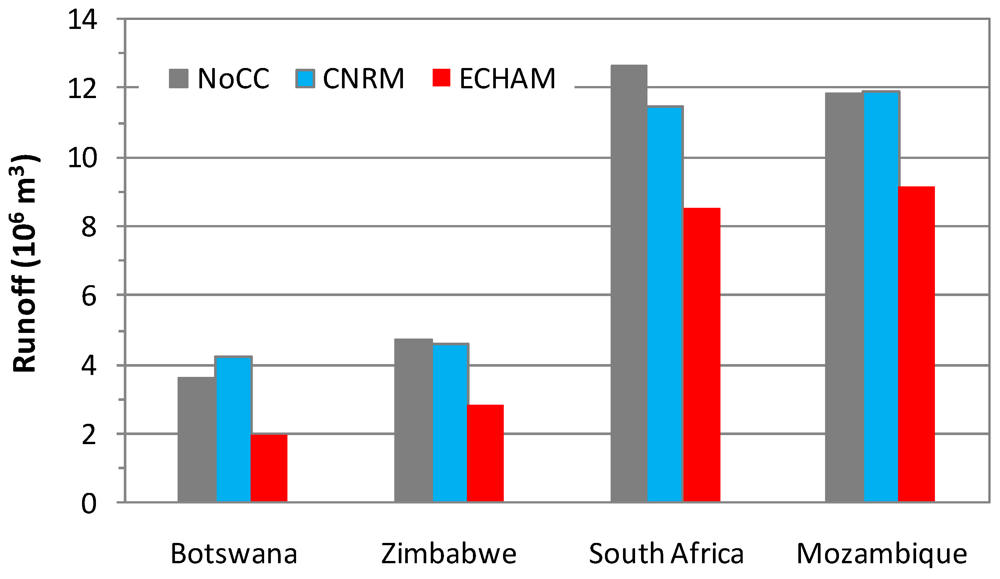
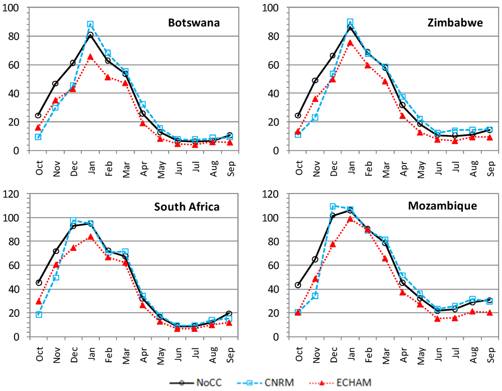
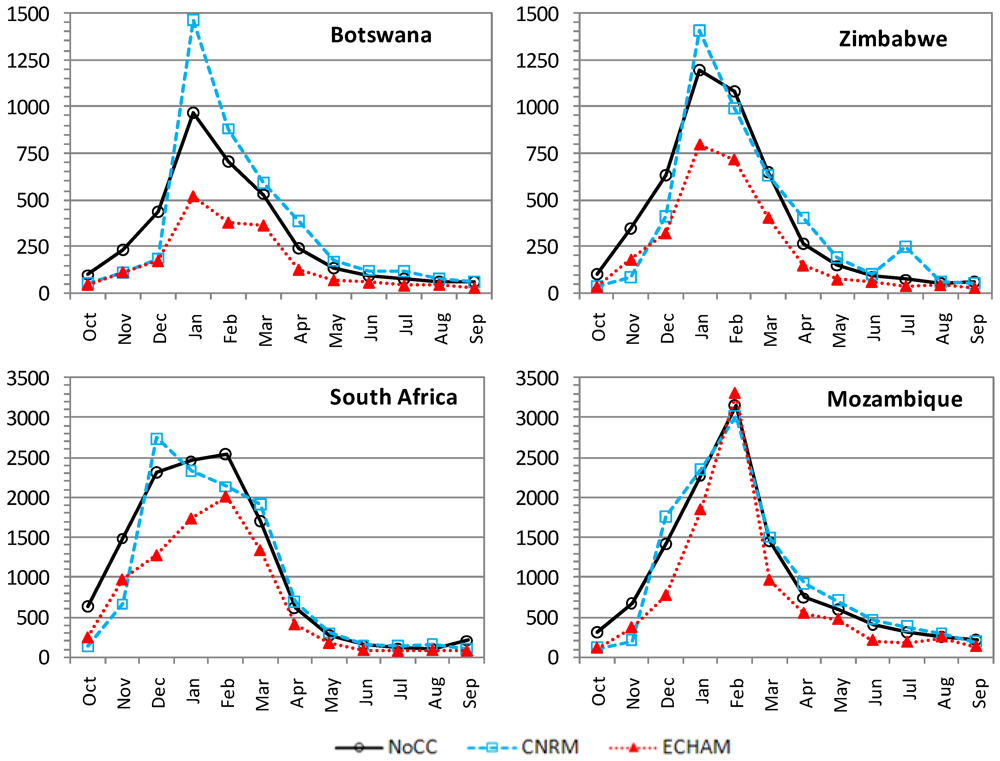
Figure 13 shows monthly mean runoff under the baseline climate and the two climate change scenarios. In Botswana, the most notable change is that in January, the peak runoff month, runoff under the CNRM scenario increases by 60 percent compared with the climate baseline. In Zimbabwe and South Africa, peak month runoff also increases. Nevertheless, in South Africa the peak runoff month comes earlier under CNRM than the climate baseline, shifting backward from February to December. Peak runoff in Mozambique actually slightly declines. For the remaining months, runoff generally decreases in spring and early summer but increases in autumn and winter under CNRM for all countries. For the ECHAM scenario, runoff universally decreases in all months across all countries, except for increases in Mozambique in February, the peak runoff month.

Figure 13. Monthly mean runoff (10⁶ m³) under the 1971–2000 climate baseline and climate change scenarios for 2050.

Figure 13. Monthly mean runoff (10⁶ m³) under the 1971–2000 climate baseline and climate change scenarios for 2050.

Decreased water availability might well result in more than just reduced water supply. De Wit and Stankiewicz found that for many African river basins a reduction in precipitation may also lead to a sharp decline in drainage density in addition to a decline in runoff [38]. This implies that many smaller rivers or their tributaries may permanently dry up due to a decline in precipitation. This particularly threatens those rural areas that lack capacity to cope with changes in runoff regimes and where the risk of loss of perennial water is high.

4.2. Irrigation Water Supply Reliability

In the WSM, irrigation water supply reliability (IWSR) is simply defined as the ratio of annual irrigation water supply to annual irrigation water demand, which represents total gross consumptive irrigation water requirements of all crops, considering “losses” by dividing total requirements by effective irrigation efficiency. Thirty IWSR values are generated for each FPU in a WSM simulation run for the thirty-year hydrological series of 1971–2000. To understand IWSR in a stochastic fashion, we conduct cumulative frequency analysis by ranking the series of IWSR values from a simulation run and deriving its non-exceedance probability distribution curve.

To analyze how IWSR will change from 2010 to 2050 without climate change impacts, we conducted water management simulations using water demands estimated for 2010 and 2050 and the hydrological data series of the 1971–2000 climate baseline or NoCC. Comparisons of simulation outcomes of 2010 and 2050 tell us how non-climatic factors such as irrigation expansion, effective irrigation efficiency improvement, water supply infrastructure development, and non-irrigation water demand growth, affect IWSR between 2010–2050. To analyze climate change impacts on IWSR for 2050, we also conducted water management simulations using the CNRM and ECHAM climate change hydrologies and the estimated 2050 water demand. Comparisons of the IWSR values under NoCC with that of CNRM and ECHAM, all at 2050, provide the impacts on IWSR from climate change alone.

The South African catchment includes most of the irrigated areas in the LRB and its current irrigated areas actually exceed its irrigation potential [8,34]. Figure 14 shows the non-exceedance probability of IWSR in the South African catchment, derived from two NoCC simulations and two climate change simulations: NoCC in 2010, NoCC in 2050, CNRM in 2050 and ECHAM in 2050. A point (x,y) chosen from any curve in Figure 14 means that the probability of IWSR being less than y equals x.

Figure 14. Non-exceedance probability of irrigation water supply reliability in the South African catchment of the Limpopo River Basin under the 1971–2000 climate baseline and two climate change scenarios for 2050.

Figure 14. Non-exceedance probability of irrigation water supply reliability in the South African catchment of the Limpopo River Basin under the 1971–2000 climate baseline and two climate change scenarios for 2050.

Figure 14 shows that water resources in the South Africa catchment of the LRB are already stressed under NoCC in 2010. For instance, the chance of IWSR being higher than 0.48 in any hydrological year type under NoCC is barely 50 percent. Projected improvements in effective irrigation efficiency and increases in irrigation infrastructure capacity (storage, withdrawal, and conveyance) are expected to improve the irrigation situation by 2050 slightly, even with irrigated areas being assumed to increase at an annual rate of 0.68 percent. The improvement is more significant in the wetter years located on the right half of the figure, indicating that increasing regulation and diversion capacities of water infrastructure can only generate limited benefits if available water resources are too scarce.

Screening alternative investment options on the basis of detailed cost-benefit analysis is out of the scope of this study. However, our scenario is based on the fact that effective irrigation efficiency improvements should be a key investment area to consider in this semi-arid region because water will remain a key input into agricultural production to feed the growing population. In addition, South Africa has the best capacity in the basin to invest in water infrastructure to improve food security and the wellbeing of rural areas.

Under the CNRM and ECHAM climate change scenarios in 2050, IWSR is significantly lower than NoCC, with the ECHAM scenario experiencing larger IWSR declines as shown in Figure 14. With increased potential evapotranspiration and reduced runoff under climate change, on the demand side, irrigated crops require more water to satisfy evapotranspiration requirement; while on the supply side, less water is actually available for irrigation due to runoff reduction and the higher priority of the competing non-irrigation users. As a result, the non-exceedance probability of IWSR being 0.45, increases from 25 percent under NoCC to 59 percent under CNRM and to 75 percent under ECHAM. The stark increases of non-exceedance probability reflect the deterioration of IWSR under climate change.

5. Conclusions

We analyzed the hydrological and irrigation water supply impacts of climate change in the LRB using a semidistributed hydrological model and the WSM water simulation module of IMPACT, based on the 1971–2000 climate baseline and the CNRM and ECHAM GCM projections for 2050 forced by SRES A1b emissions. Significant reductions of annual precipitation in 2050 are found in all countries for both climate change scenarios, compared with the climate baseline. The most pronounced precipitation decline occurs in October and November under the moderate dry CNRM scenario, while precipitation declines in nearly all months under the very dry ECHAM scenario. Although annual mean precipitation universally decreases, peak month precipitation increases for all countries under the moderately dry CNRM scenario. Even under the very dry ECHAM scenario, precipitation increases in the peak rainfall month in Mozambique. Thus, while annual totals are reduced, flooding might increase in flood-prone areas.

PET increases in all riparian countries under both the CNRM and ECHAM climate change scenarios, with most increases occurring in spring and early summer. This suggests that under climate change more water is needed by crops in their planting and early growing stages in the basin. We found major annual runoff reductions in all riparian countries under the very dry ECHAM scenario. Under the moderately dry CNRM scenario, however, annual runoff declines in Zimbabwe and South Africa but slightly increases in Botswana and Mozambique, even though annual precipitation decreases in all countries. Notably, peak month runoff increases in all countries except for Mozambique under the CNRM scenario. This indicates that the intra-annual distribution of precipitation has a strong influence on runoff.

The WSM simulations reveal that IWSR in 2050 declines significantly under both climate change scenarios compared with the climate baseline, even though IWSR values increase from 2010 to 2050 under baseline climate due to infrastructure and management improvement. Climate change-induced IWSR declines, add an additional constraint for future irrigation development in the basin. Even small, permanent changes in precipitation patterns need to be incorporated into water resource and agricultural planning as they will require changes in crop varieties, planting dates, and cropping patterns, placing new requirements on both agricultural research and development and extension services. Assessing hydrological impacts of climate change is crucial given that expansion of irrigated areas has been postulated as one key adaptation strategy for Sub-Saharan Africa. Such expansion will need to take into account changes in availability of water resources in African river basins.

References

- Trenberth, K.E.; Jones, P.D.; Ambenje, P.; Bojariu, R.; Easterling, D.; Klein Tank, A.; Parker, D.; Rahimzadeh, F.; Renwick, J.A.; Rusticucci, M.; et al. Observations: Surface and atmospheric climate change. In Climate Change 2007: The Physical Science Basis. Contribution of Working Group I to the Fourth Assessment Report of the Intergovernmental Panel on Climate Change; Solomon, S., Qin, D., Manning, M., Chen, Z., Marquis, M., Averyt, K.B., Tignor, M., Miller, H.L., Eds.; Cambridge University Press: Cambridge, UK and New York, NY, USA, 2007. [Google Scholar]
- Zhu, T.; Jenkins, M.W.; Lund, J.R. Estimated impacts of climate warming on California water availability under twelve future climate scenarios. J. Am. Water Resour. Assoc. 2005, 41, 1027–1038. [Google Scholar] [CrossRef]
- Arnell, N.W. Climate change and global water resources: SRES emissions and social-economic scenarios. Glob. Environ. Change 2004, 14, 31–52. [Google Scholar] [CrossRef]
- Rogers, P. Coping with global warming and climate change. J. Water Resour. Plan. Manag. 2010, 134, 203–204. [Google Scholar] [CrossRef]
- IPCC, Summary for policymakers. In Climate Change 2007: Impacts, Adaptation and Vulnerability. Contribution of Working Group II to the Fourth Assessment Report of the Intergovernmental Panel on Climate Change; Parry, M.L.; Canziani, O.F.; Palutikof, J.P.; van der Linden, P.J.; Hanson, C.E. (Eds.) Cambridge University Press: Cambridge, UK, 2007; pp. 7–22.
- Kundzewicz, Z.W.; Mata, L.J.; Arnell, N.W.; Döll, P.; Kabat, P.; Jiménez, B.; Miller, K.A.; Oki, T.; Sen, Z.; Shiklomanov, I.A. Freshwater resources and their management. In Climate Change 2007: Impacts, Adaptation and Vulnerability. Contribution of Working Group II to the Fourth Assessment Report of the Intergovernmental Panel on Climate Change; Parry, M.L., Canziani, O.F., Palutikof, J.P., van der Linden, P.J., Hanson, C.E., Eds.; Cambridge University Press: Cambridge, UK, 2007; pp. 173–210. [Google Scholar]
- Brown, C.; Lall, U. Water and economic development: The role of variability and a framework for resilience. Nat. Resour. Forum 2006, 30, 306–317. [Google Scholar] [CrossRef]
- FAO, Drought Impact Mitigation and Prevention in the Limpopo River Basin: A Situation Analysis; Land and Water Discussion Paper No. 40; Food and Agriculture Organization of the United Nations: Roma, Italy, 2004.
- CPWF, Limpopo Basin Profile: Strategic Research for Enhancing Agricultural Water Productivity; Challenge Program on Water and Food: Colombo, Sri Lanka, 2003.
- Reason, C.J.C.; Hachigonta, S.; Phaladi, R.F. Interannual variability season characteristics over the Limpopo region of Southern Africa. Int. J. Climatol. 2005, 25, 1835–1853. [Google Scholar] [CrossRef]
- IWMI, IDIS (Integrated Data Information System) Basin Kit— Limpopo Basin V 1.0 (CD-ROM); International Water Management Institute: Colombo, Sri Lanka, 2006.
- Mitchell, T.D.; Jones, P.D. An improved method of constructing a database of monthly climate observations and associated high-resolution grids. Int. J. Climatol. 2005, 25, 693–712. [Google Scholar] [CrossRef]
- Zhu, T.; Ringler, C.; Rosegrant, M.W. Development and Validation of a Global Hydrology Model for Climate Change Impact Assessment; International Food Policy Research Institute: Washington, DC, USA, 2010; Photocopy. [Google Scholar]
- Rosegrant, M.W.; Cai, X.; Cline, S.A. World Water and Food for 2025: Dealing with Scarcity; International Food Policy Research Institute: Washington, DC, USA, 2002. [Google Scholar]
- Rosegrant, M.W.; Msangi, S.; Ringler, C.; Sulser, T.B.; Zhu, T.; Cline, S.A. International Model for Policy Analysis of Agricultural Commodities and Trade (IMPACT): Model Description; International Food Policy Research Institute: Washington, DC, USA, 2008. [Google Scholar]
- Priestley, C.H.B.; Taylor, R.J. On the assessment of surface heat flux and evaporation using large scale parameters. Mon. Weather Rev. 1972, 100, 81–92. [Google Scholar]
- Shuttleworth, W.J. Evaporation. In Handbook of Hydrology; Maidment, D.R., Ed.; McGraw-Hill: New York, NY, USA, 1993. [Google Scholar]
- Zhao, R.J. The Xinanjiang model applied in China. J. Hydrol. 1992, 135, 371–381. [Google Scholar] [CrossRef]
- Wood, E.F.; Lettenmaier, D.P.; Zartarian, V.G. A land-surface hydrology parametrization with subgrid variability for general circulation models. J. Geophys. Res. 1992, 97, 2717–2728. [Google Scholar]
- Arnell, N.W. A simple water balance model for the simulation of streamflow over a large geographic domain. J. Hydrol. 1999, 217, 314–335. [Google Scholar] [CrossRef]
- Chow, V.T.; Maidment, D.R.; Mays, L.W. Applied Hydrology; McGraw-Hill: New York, NY, USA, 1988. [Google Scholar]
- Doll, P.; Kaspar, F.; Lehner, B. A global hydrological model for deriving water availability indicators: Model tuning and validation. J. Hydrol. 2003, 270, 105–134. [Google Scholar] [CrossRef]
- Alcamo, J.; Doll, P.; Henrichs, T.; Kaspar, F.; Lehner, B.; Rosch, T.; Siebert, S. Development and testing of the WaterGAP2 global model of water use and availability. Hydrol. Sci. J. 2003, 48, 317–337. [Google Scholar] [CrossRef]
- Goldberg, D.E. Genetic Algorithms in Search, Optimization, and Machine Learning; Kluwer Academic Publishers: Boston, MA, USA, 1989. [Google Scholar]
- Nash, J.E.; Sutcliffe, J.V. River flow forecasting through conceptual models part I—A discussion of principles. J. Hydrol. 1970, 10, 282–290. [Google Scholar] [CrossRef]
- Keller, A.; Keller, J.; Seckler, D. Integrated Water Resource Systems: Theory and Policy Implications; Research Report 3; International Water Management Institute: Colombo, Sri Lanka, 1996. [Google Scholar]
- Cai, X.; Rosegrant, M.W. Optional water development strategies for the Yellow River Basin: Balancing agricultural and ecological water demands. Water Resour. Res. 2004, 40. [Google Scholar]
- Falkenmark, M.; Rockström, J. The new blue and green water paradigm: Breaking new ground for water resources planning and management. J. Water Resour. Plan. Manag. 2006, 132, 129–132. [Google Scholar] [CrossRef]
- Christensen, J.H.; Hewitson, B.; Busuioc, A.; Chen, A.; Gao, X.; Held, R.; Jones, R.; Kolli, R.; Kwon, W.; Laprise, R.; et al. Regional climate projections. In Climate Change 2007: The Physical Science Basis. Contribution of Working Group I to the Fourth Assessment Report of the Intergovernmental Panel on Climate Change; Solomon, S., Qin, D., Manning, M., Chen, Z., Marquis, M., Averyt, K.B., Tignor, M., Miller, H.L., Eds.; Cambridge University Press: Cambridge, UK and New York, NY, USA, 2007. [Google Scholar]
- Mote, P.; Brekke, L.; Duffy, P.B.; Maurer, E. Guidelines for constructing climate scenarios. Eos Trans. AGU 2011, 92, 257–258. [Google Scholar] [CrossRef]
- IPCC (Intergovernmental Panel on Climate Change), Emissions Scenarios 2000: Special Report of the Intergovernmental Panel on Climate Change; Cambridge University Press: Cambridge, UK, 2000.
- Jones, P.G.; Thornton, P.K.; Heinke, J. Generating Characteristic Daily Weather Data Using Downscaled Climate Model Data from the IPCC’s Fourth Assessment; Project Report. 2009. Available online: http://dspacetest.cgiar.org/handle/10568/2482 (accessed on 16 January 2011).
- Gerald, N.; Rosegrant, M.W.; Palazzo, A.; Gray, I.; Ingersoll, C.; Robertson, R.; Tokgoz, S.; Zhu, T.; Sulser, T.; Ringler, C.; et al. Food security, Farming,and Climate Change to 2050; Research Monograph, International Food Policy Research Institute (IFPRI): Washington, DC, USA, 2010. [Google Scholar]
- FAO, Irrigation Potential in Africa: A Basin Approach; FAO Land and Water Bulletin 4; Food and Agriculture Organization of the United Nations: Roma, Italy, 1997.
- You, L.; Wood, S. An entropy approach to spatial disaggregation of agricultural production. Agric. Syst. 2006, 90, 329–347. [Google Scholar] [CrossRef]
- Portmann, F.T.; Siebert, S.; Döll, P. MIRCA2000—Global monthly irrigated and rainfed crop areas around the year 2000: A new high-resolution data set for agricultural and hydrological modeling. Glob. Biogeochem. Cycles 2010, 24. [Google Scholar]
- FAO. FAOSTAT-Crops; Food and Agriculture Organization of the United Nations: Rome, Italy. Available online: http://faostat.fao.org (accessed on 6 October 2010).
- De Wit, M.; Stankiewicz, J. Changes in surface water supply across Africa with predicted climate change. Science 2006, 301, 1917–1921. [Google Scholar]
© 2012 by the authors; licensee MDPI, Basel, Switzerland. This article is an open-access article distributed under the terms and conditions of the Creative Commons Attribution license (http://creativecommons.org/licenses/by/3.0/).
Share and Cite
MDPI and ACS Style
Zhu, T.; Ringler, C. Climate Change Impacts on Water Availability and Use in the Limpopo River Basin. Water 2012, 4, 63-84. https://doi.org/10.3390/w4010063
AMA Style
Zhu T, Ringler C. Climate Change Impacts on Water Availability and Use in the Limpopo River Basin. Water. 2012; 4(1):63-84. https://doi.org/10.3390/w4010063
Chicago/Turabian StyleZhu, Tingju, and Claudia Ringler. 2012. "Climate Change Impacts on Water Availability and Use in the Limpopo River Basin" Water 4, no. 1: 63-84. https://doi.org/10.3390/w4010063