2.1. Site Description and Design Characteristics
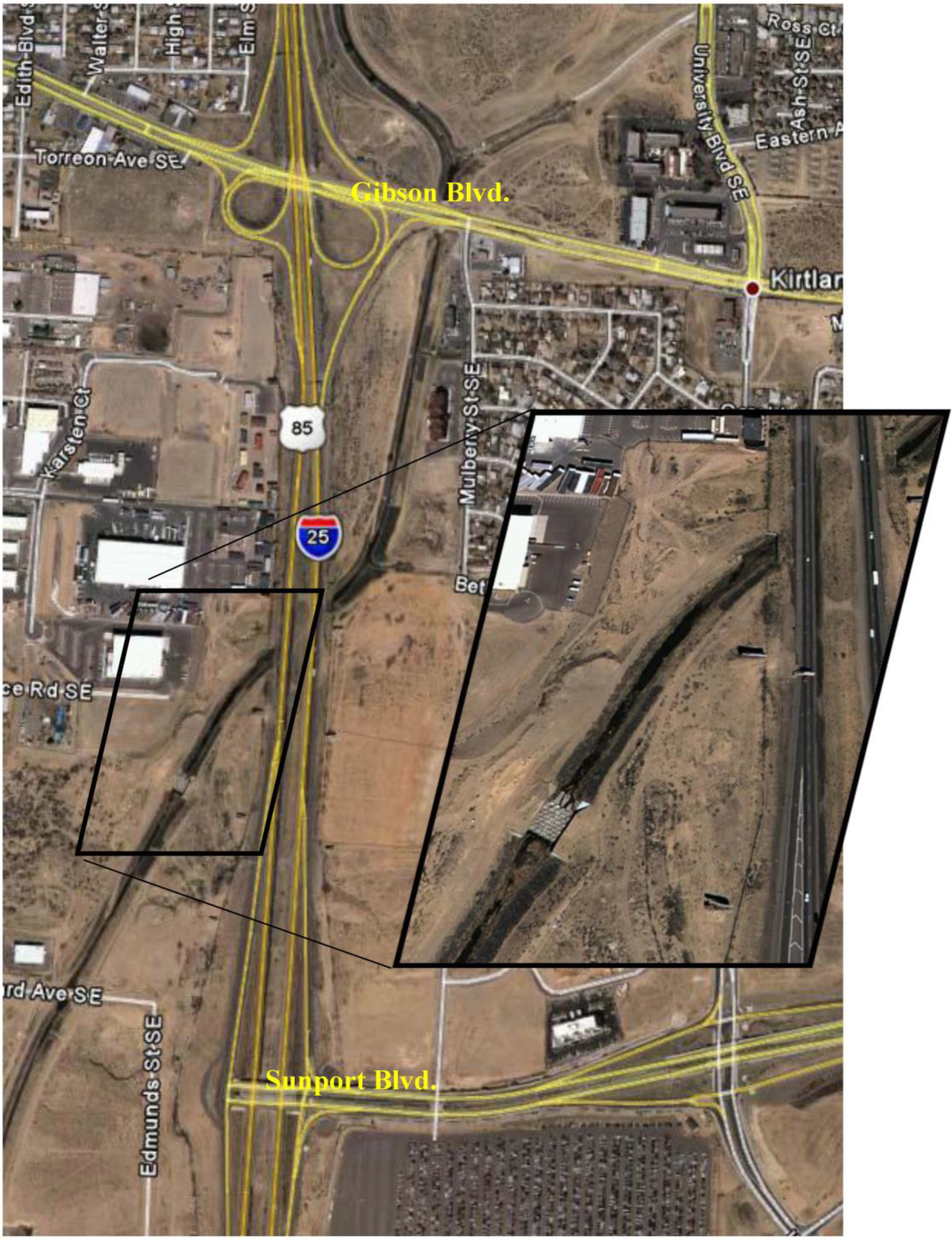
SDC is one of the main storm-water collectors in Albuquerque. The upstream portion of AMAFCA’s SDC collects storm-water runoff from the area east of Interstate 25 and south of the University of New Mexico area. SDC receives storm water from storm-water drains, the Genievas Arroyo, and the Kirtland Arroyo before crossing Interstate 25. A concrete baffle chute is located on the channel approximately 240 m downstream of its Interstate 25 crossing (
Figure 3).
Figure 3.
Image map of the project site.
Figure 3.
Image map of the project site.
SDC is a trapezoidal channel with an earthen bottom width of 9.0 m and riprap side slopes with a vertical (
V)/horizontal (
H) ratio of 1:2. The channel has a longitudinal slope of 0.14% just upstream of the baffle chute. The Manning roughness coefficient of the channel is estimated to be 0.035. Although the channel has been designed for a discharge of 97.70 m
3/s, the more frequent discharges in the channel vary between 3 and 16 m
3/s. All the reported data were obtained from initial design reports which are available in the AMAFCA office.
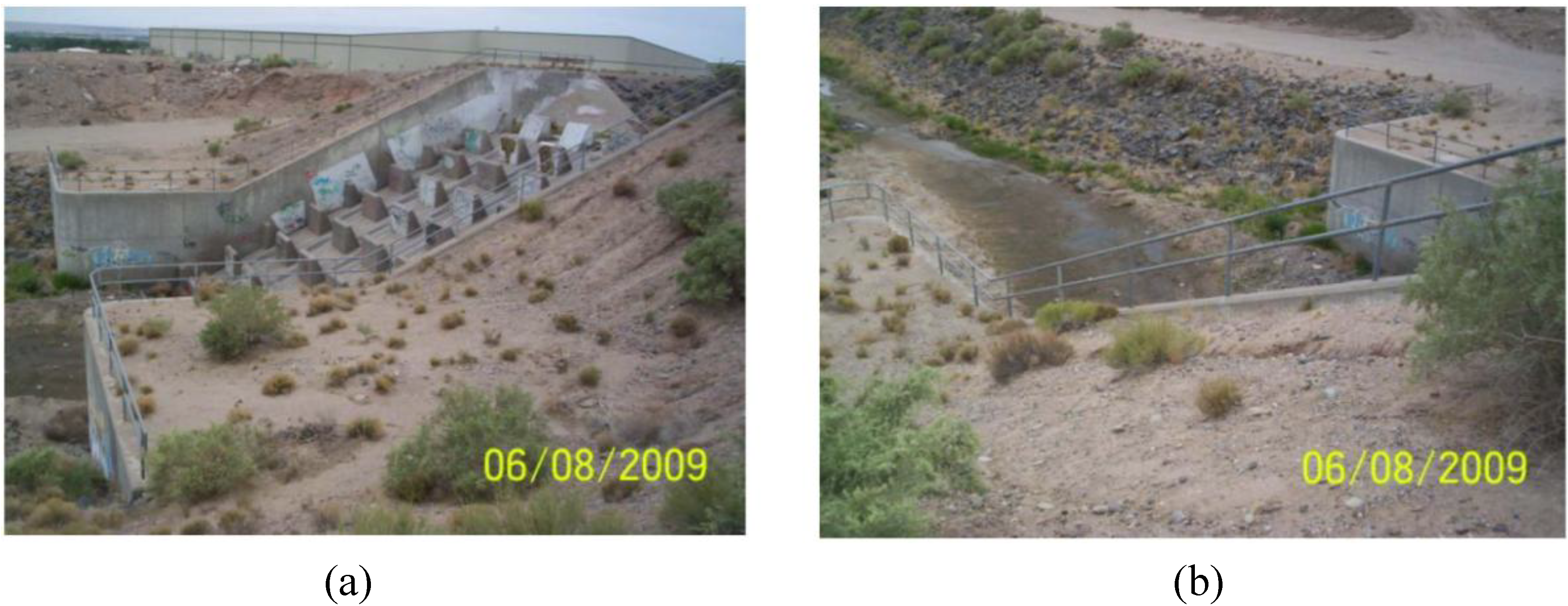
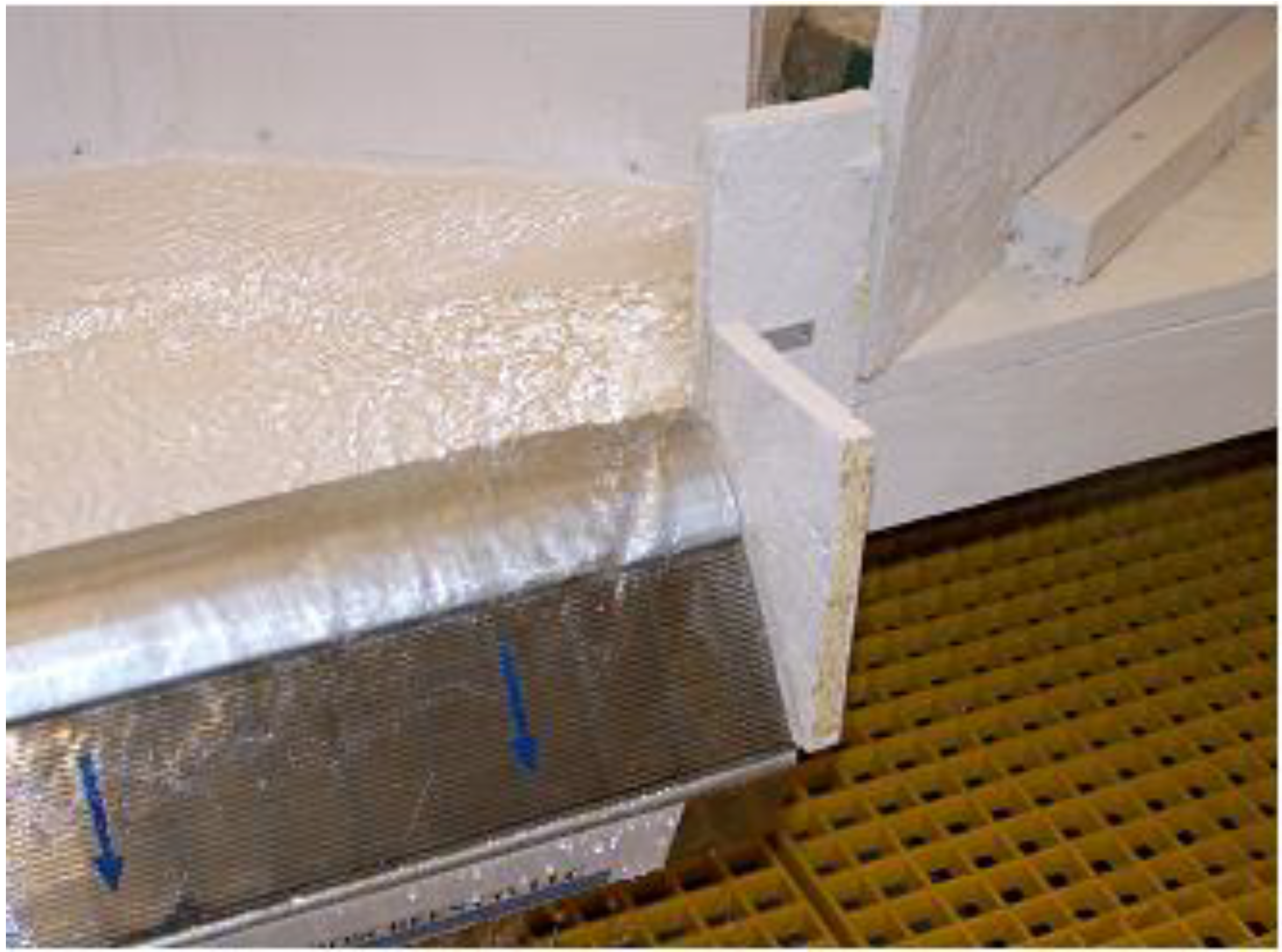
Figure 4 shows different views of the channel and baffle chute. They depict the existing condition of the channel.
Figure 4a shows a general view of the baffle chute while the SDC is also observed at downstream and upstream of the baffle chute.
Figure 4b refers to the downstream condition of the baffle chute and existing condition of the SDC.
Figure 4.
Photos depicting the existing condition of the SDC and baffle chute, (a)-general view and (b)-downstream condition.
Figure 4.
Photos depicting the existing condition of the SDC and baffle chute, (a)-general view and (b)-downstream condition.
AMAFCA’s objective is to divert flow at the upstream end of the existing concrete structure and remove debris from this flow before allowing it to re-enter the SDC.
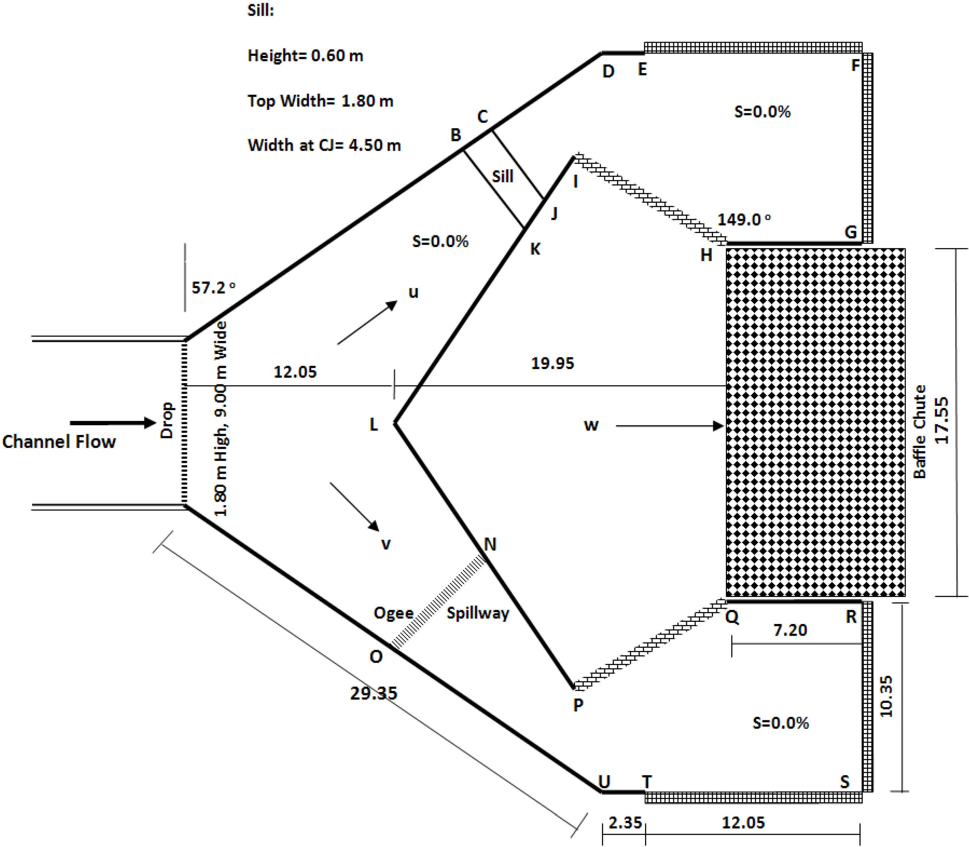
Figure 5 depicts the general layout for one the design alternatives considered in this project. The cross-hatched area shows the designed location for screens to remove floating debris under the designed flow rates. The inflow discharge and the depth and velocity behind the screens and the Froude number are the main variables that determine the required length and width of the screens—the two parameters that directly affect the cost of the screen setup. The proposed geometry for the diversion structure including the screen setup is based on scientific and technical reasons. In this design, the settlement of suspended sediments, easy access to the sediment deposition zone and screens, economy of the design, and hydraulic performance of the system had been considered. These factors are necessary for providing a suitable ground to remove the trapped floating debris and sediments from the site, reduce the cost, and create a uniform distribution of flow around the screens. Among these, the final item can also help in determining variables necessary to design the screen dimensions, which can lead to an optimum and cost-effective design of the screen. In the initial design, the two 10.50 m walls (
HI and
PQ) are the existing wing walls that remain fixed. Except for the 1.80 m drop structure at the beginning, sill and ogee spillway, the bottoms of all other parts of the diversion structure up to the screens are at the same level. The following paragraphs describe different design components.
Starting from upstream, while the main direction of existing flow is to the baffle chute, flow is blocked and diverted to the left and right directions towards the screens. The idea is to divert the first 15.49 m3/s to the left direction and the next 15.49 m3/s up to 30.98 m3/s to the right direction. Flows higher than 30.98 m3/s must flow to the baffle chute in the original direction of flow. A 1.8 m high and 9.0 m wide drop structure has been considered at the confluence of the channel with the diversion structure. In addition to its role in local energy dissipation, the main advantage of this drop structure is that it reduces any backwater effect resulting from the placement of this diversion structure. A broad-crested weir (sill) with a height of 0.6 m and top width of 1.8 m was considered for the left direction. Another structure that was considered is an ogee spillway on the right side. This spillway prevents the first 15.49 m3/s flow from going to the right direction, and its height and width must be adjusted by taking this into consideration. Both the left and the right sides must have the capacity to convey a total discharge of 30.98 m3/s. Discharges higher than 30.98 m3/s up to 97.7 m3/s must flow in the main direction of the flow towards the baffle chute. This requires that a weir or a spillway be used along the KLN section. Although the end points of the KLN section are connected to the sill and ogee spillway and the width of this section is fixed depending on the location of the ogee spillway on the right, the height along KLN must be adjusted to function properly. Two sluice gates were considered for the sill and ogee spillway. These two gates add flexibility to the design. The first sluice gate, which is related to the sill, allows the operator to adjust the flow to nearly 15.49 m3/s to the left at higher discharges; the second sluice gate, which is related to the ogee spillway, functions similarly to adjust flows of nearly 15.49 m3/s to the right side. Flow rates higher than 97.7 m3/s and even 15.49 m3/s are less frequent and not very important in terms of debris removal. The zone behind the sill and spillways can act as a settling basin to settle the suspended sediments.
Figure 5.
Layout and main dimensions of the design in meters.
Figure 5.
Layout and main dimensions of the design in meters.
The complicated nature of the flow is evident in this design. Many factors such as the geometry and topography contribute to this complexity, which makes it necessary to use appropriate analysis tools such as physical and numerical modeling in addition to classical design methods.
Although the mechanisms used to divert flow are briefly discussed, this study focused on flow observation and detailing in the zone behind the C-S. The Delft3D-FLOW numerical model, which is a commercially available software program, and physical modeling were used to achieve this. Although the existence of floating debris and sediments can affect water properties and flow behaviour, such secondary effects were ignored for urban water system considered in this study. Therefore, both physical and numerical models were developed for clear water condition.
2.2. Physical Model Setup
With reference to the explained design features depicted in
Figure 5, two main specific objectives were considered for the physical model:
(1) To observe flow patterns for different specified flow rates around C-Ss and provide some depth measurements at specific locations to estimate physical parameters for the simple CFD model used in this study. Although numerical modeling can produce detailed information about the flow pattern, velocity, and depth around a C-S, there are aspects of the flow that need further clarification, and observation in the physical model was quite useful in this regard.
(2) To observe flow patterns at the point of diversion and extract necessary data for designing the height and width of the ogee spillways along the ON and KLN sections. Although such designs can be made by using available classical methods, the use of such an inexpensive physical model can further validate standard designs, especially for the shaped ogee spillway along KLN with the proposed geometry.
The existing trapezoidal channel at the Civil Engineering Department Hydraulics Laboratory, University of New Mexico was used to build the physical model.
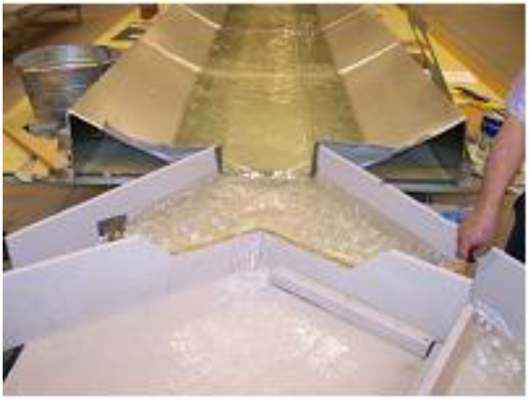
Figure 6 shows a general configuration of the sheet metal channel with a bottom width of 0.3 m and side slopes of 2:1 (H:V). The longitudinal slope can be adjusted. A 1/30 scale allowed for use of the existing channel (0.3 m bottom width of the modeled channel = 9.0 m bottom width of the prototype channel) and was appropriate for the pump capacity to produce the different discharges necessary in the study. All discharges developed at this scale were also measurable volumetrically using 18- and 4-gallon containers and a stop watch. The maximum relative error in discharge measurement was estimated to be 5% and 2.5% for high and low discharges considered in this study. Considering the existence of a 0.06 m drop in the beginning of the modeled diversion structure, we decided to build the model off the flume table right at the end of the flume. The legs of the modeling table were adjustable using screws, which made it possible to have a flat bottom at the desired elevation. The Froude number similitude for open-channel, free-surface flows was used to determine the similitude relationships between the model and the prototype variables and to convert modeling values to the corresponding prototype values. Physical modeling activities were organized in two steps to achieve the two main objectives of the study.
Figure 6.
Picture showing the general configuration of the flume and physical model.
Figure 6.
Picture showing the general configuration of the flume and physical model.
In the first step, half of the model was built.
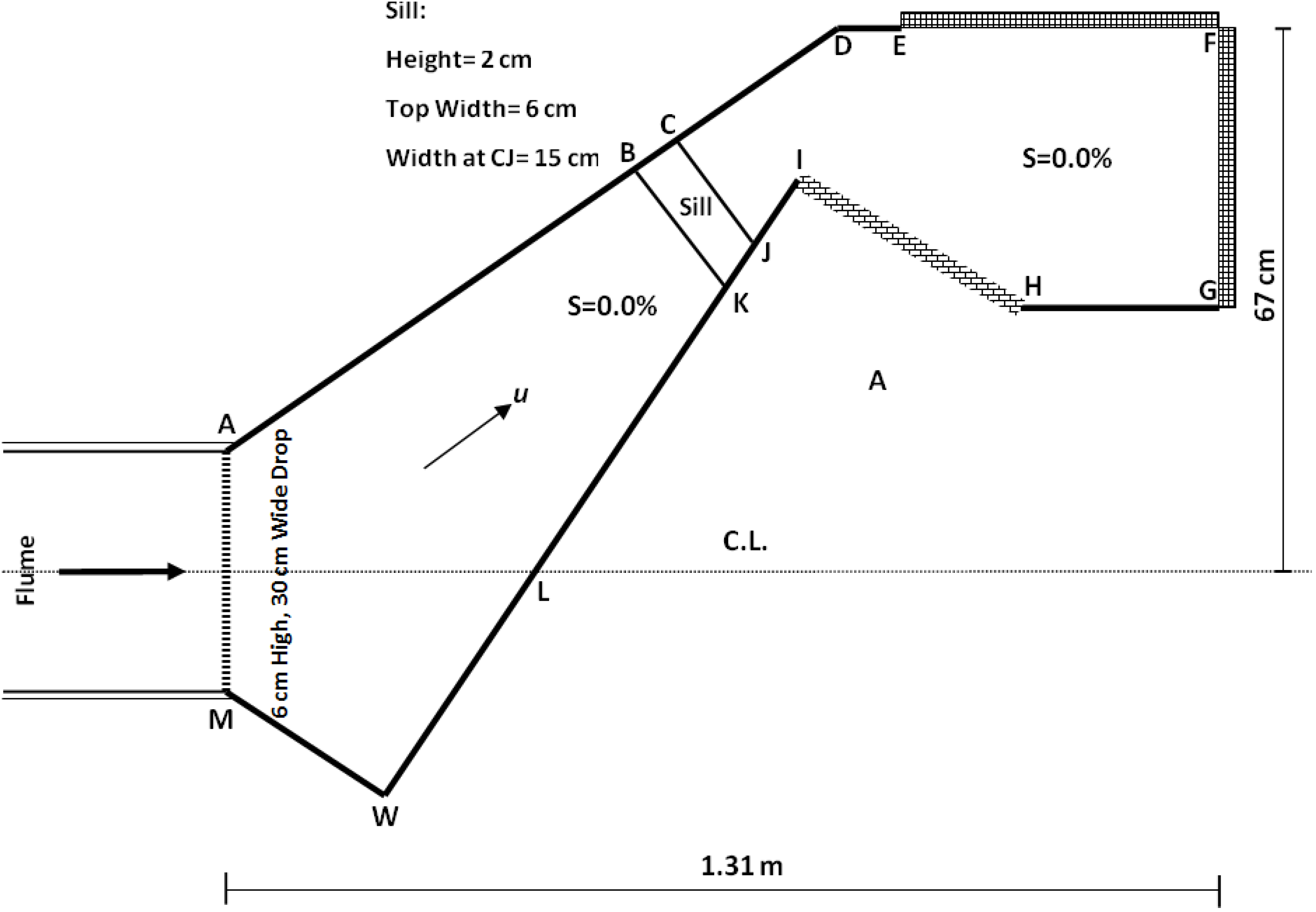
Figure 7 shows a sketch of this setup whose major dimensions were determined from
Figure 5 on the basis of the 1/30 scale of the model. It is worth mentioning that the slope of the flume did not have an important role in this study because the flow pattern after the drop and, more specifically, after, the sill was the centre of focus, and the flow was governed either by the critical condition at the drop or depth at the sill. Both the model and prototype were turbulent. The physical modeling activity was to run different flows (0.686 L/s corresponding to 3.38 m
3/s in prototype) and high discharges (3.142 L/s corresponding to 15.49 m
3/s in prototype) through the system, observe the flow pattern at different zones of interest, and measure depth at some key locations. The effect of using a smooth curved wall at point
D was also studied in this case. Since the same scenarios were also produced in the numerical model, further details about the scenarios are given in the numerical modeling section (
Section 2.3) and results and discussion (
Section 3).
Figure 7.
Extent and dimensions of the physical model.
Figure 7.
Extent and dimensions of the physical model.
In the second step, the physical model was built to be almost complete; it included the
v and
w directions of flow, as shown in
Figure 5. This setup was used to adjust the height of different spillways along sections
NO and
KLN. The main objective of this paper is to study the flow behind and around the C-Ss or after the sill, as shown in
Figure 7, using the first step of physical and numerical modeling. Therefore, the procedure for adjusting the spillway heights is briefly introduced here, and major dimensions are given.
The width of section NO for building ogee weir was considered to be 0.25 m. This selection was based on the balance between providing an appropriate zone for sediment deposition and increasing the width of the spillway to reduce any backwater effect. To adjust the height of the weir along NO, a discharge of 3.142 L/s (corresponding to 15.49 m3/s in the prototype) was run through the system; with no flow in the v and w directions, the height of the ogee spillway was found to be 0.08 m. An ogee-shaped spillway was considered along section KLN. The triangular shape increased the effective length of the spillway and thus reduced the backwater effect on the flow in the channel. It also helped in dissipating energy downstream of the spillway when the flow jets hit each other. The lengths of section KLN are 0.45 and 0.30 m in the KL and LN parts, respectively; they have a total length of 0.75 m. To adjust the heights along KLN, a discharge of 6.284 L/s was run through the system. A gate was installed at the sill. The opening of the gate was controlled to let nearly 3.142 L/s run in the u direction and another 3.142 L/s run in the v direction towards the weir along the NO section. Observations and measurements made behind the weirs showed that the required heights at points K, L, and N were 0.115, 0.121 and 0.117 m, respectively. These numbers indicate a sloped condition along KLN. Observations showed that this condition provided a more uniform distribution of flow along the section. All the physical model length, width, and height numbers can be converted to prototype values if multiplied by 30. Although no manual operation is required for discharges less than 15.49 m3/s, this design also indicates a need for a gate at the sill to adjust the flow rate in both directions for discharges between 15.49 and 30.98 m3/s. Obviously, for less frequent discharges of more than 30.98 m3/s when the KLN spillway is also operating, a control gate is required above the NO spillway for adjusting the flow rate in different directions. In general, while these two control gates add flexibility to the design, there is a need to manually operate them in the field under high but less frequent discharges. The gate openings were also adjusted.
2.3. Numerical Model Setup
Commercial CFD software is widely used in engineering design. It has the advantage of comprehensive validation against many hypothetical and laboratory test cases, a graphical user interface, and a large number of different models for physical phenomena, such as the representation of turbulence. In hydraulics and river engineering works, CFD can be used in different ways including as a method for improving conveyance estimation to enhance one-dimensional and two-dimensional models, as a technique for assessing the performance of small-scale river engineering works and hydraulic structures such as river intakes/outtakes, weirs, fish passes and sluice gates, and as a scientific tool for developing understanding of the fundamental fluid dynamics of flow in rivers [
3].
Considering that most CFD codes have been developed for mechanical engineering works, the application of CFD to hydraulic problems raises a number of issues related to geometry, free surface, boundary conditions, hydraulic roughness, flow regime and turbulence [
3].
Delft3D-FLOW is a commercial software program available from WL|Delft Hydraulics (now Deltares) and was used in this study. Delft3D-FLOW is the hydrodynamic module of Delft3D, which is WL|Delft Hydraulics’ fully integrated program for modeling water flows, waves, water quality, particle tracking, ecology, sediment and chemical transport, and morphology. Its capability for modeling subcritical-supercritical free surface flows, handling different types of boundary conditions, and availability of different turbulence models made the model suitable for use in this study. Mesh generation capabilities and bathymetry or topography generation are other powerful features available in this software. In addition, a trial version of the model with some technical support from the model provider made the model a good candidate for use in this study.
The following is a brief description of the model related to this study, as drawn from the user manual for Delft3D-FLOW [
4]. Delft3D-FLOW is a multi-dimensional (2D or 3D) hydraulic (and transport) simulation model; it essentially solves the Navier-Stokes equations for incompressible fluid under shallow water and Boussinesq assumptions. In the vertical momentum equation, the vertical acceleration is neglected, which leads to the hydrostatic pressure distribution. In 3D models, the vertical velocities are computed from the continuity equation. The set of partial differential equations in combination with an appropriate set of initial and boundary conditions is solved on a finite difference staggered grid. In the horizontal direction, Delft3D-FLOW uses structured orthogonal curvilinear coordinates. Both Cartesian and spherical coordinates are supported. In the vertical direction, Delf3D-FLOW offers two different vertical grid system, the
coordinate system (
-grid) and the Cartesian coordinate system (Z-grid). In the
-grid, the vertical grid consists of layers bounded by two sigma planes; these are not strictly horizontal but follow the bottom topography and free surface. Because the
-grid is boundary-fitted both to the bottom and to the moving free surface, a smooth representation of the topography is obtained. In order to capture non-hydrostatic flow phenomena in special cases, the hydrostatic version of the Cartesian grid (Z-model), which is part of the Delft3D modeling suite, has been extended with a non-hydrostatic module.
In this study, the idea was to keep the structure of the model as simple as possible without a serious need to calibrate parameters. Meanwhile, observations in the physical model showed that the flow has a high width to depth ratio especially around the C-Ss. Therefore, the 2D depth-averaged model of Delf3D-FLOW in a one-layer
-grid system was used to model the flow system shown in
Figure 5 and
Figure 7. This model can provide a reasonable distribution of depth and velocity field required in this study. The numerical model was developed for the full or prototype scale of the flow system for the geometry shown in
Figure 7. Developing the model for the prototype scale made the modeling results directly available for use in design and analysis.
Similar to any conventional numerical model development, the following steps, which correspond to the Delft3D-FLOW graphical user interface menu and module setup, were followed.
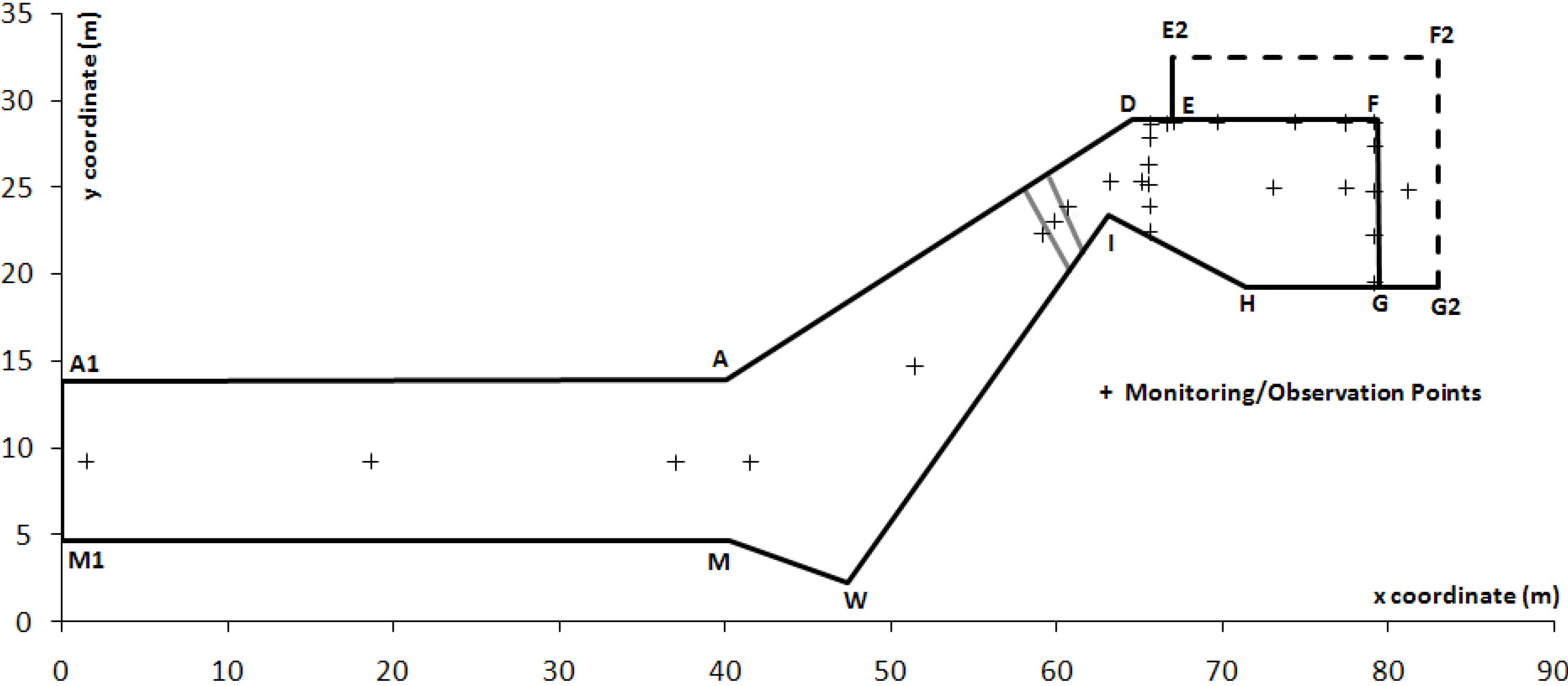
(1) First, the extent of the area to be modeled was selected; this includes the definition of the location and extent of open boundaries and the land-water boundary. Although
Figure 7 presents the domain of the problem at hand, two boundaries
E2-F2 and
F2-G2, which are shown in
Figure 8, were artificially defined to model the free overfall over the boundaries
EF and
FG. In other words, the bathymetry and water levels at boundaries
E2-F2 and
F2-G2 were defined so low that a free overfall could occur at boundaries
EF and
FG.
Figure 8 also shows the monitoring/observation points whose information were extracted and used in analysis.
Figure 8.
Modeled area and monitoring/observation points.
Figure 8.
Modeled area and monitoring/observation points.
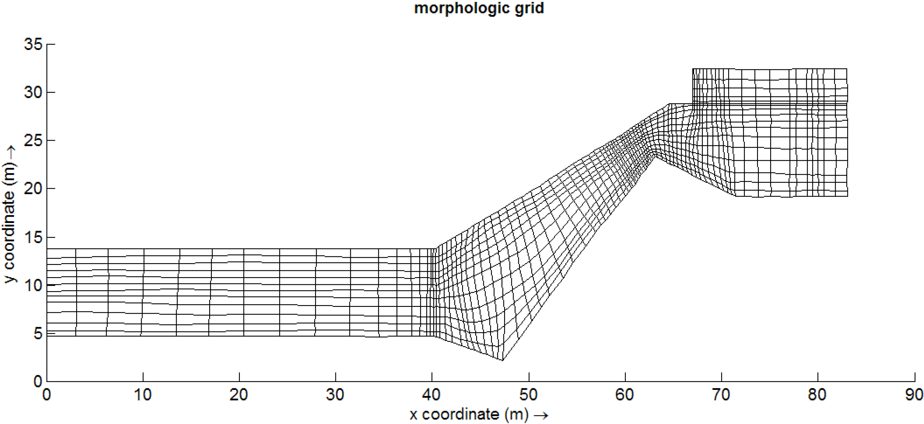
(2) The numerical grid shown in
Figure 9 was generated, and bathymetry was defined on the numerical grid. These were done using modules available in the software. The generated grid is the result of a trial-and-error procedure for selecting optimum parameters for grid size and distribution. In doing so, by covering the geometry and well-defined angles in the horizontal plane, higher resolutions near the zones of interest for flow analysis and in areas with sudden changes in bed topography (e.g., drop locations) were considered. The bathymetry was developed from a set of given sampled data from the bed elevation using interpolation techniques available in the bathymetry module of the software. Sharp changes in the bed elevation at locations such as drops were accurately captured in the generated bathymetry. This was achieved by using visualization capabilities in the modules that help in detecting any anomaly in geometry and bathymetry. In brief, with respect to a horizontal plane of reference, the bed elevations in the inflow section (
A1-M1 in
Figure 8), just upstream the drop
AM, just downstream the drop
AM, above the sill, right at the crest of the drops
EF and
FG and at artificially defined boundaries
E2-F2 and
F2-G2 are 12.03, 11.99, 10.19, 10.79, 10.19 and 6.00 m, respectively. This information is helpful in interpreting water level data.
Figure 9.
Grid used for numerical analysis.
Figure 9.
Grid used for numerical analysis.
(3) Different flow scenarios corresponding to the objectives of the study and physical model measurements were considered.
Table 1 presents these scenarios with some basic descriptions. It should be considered that the selected downstream water levels along
E2-F2 and
F2-G2 boundaries, which correspond to small depth values of 0.2 m and 0.1 m, for high and low discharges, respectively, do not affect the results in the areas of interest.
Table 1.
Different flow scenarios.
Table 1.
Different flow scenarios.
| Description/design variable | High discharge | Low discharge |
|---|
| Sharp | Curved | Curved with vane | Sharp | Curved | Curved with vane |
|---|
| Acronym | HDS a | HDC | HDCV | LDS | LDC | LDCV |
| Discharge (m3/s) | 15.49 | 15.49 | 15.49 | 3.38 | 3.38 | 3.38 |
| Downstream water level along E2-F2 and F2-G2 boundaries (m) | 6.2 | 6.2 | 6.2 | 6.1 | 6.1 | 6.1 |
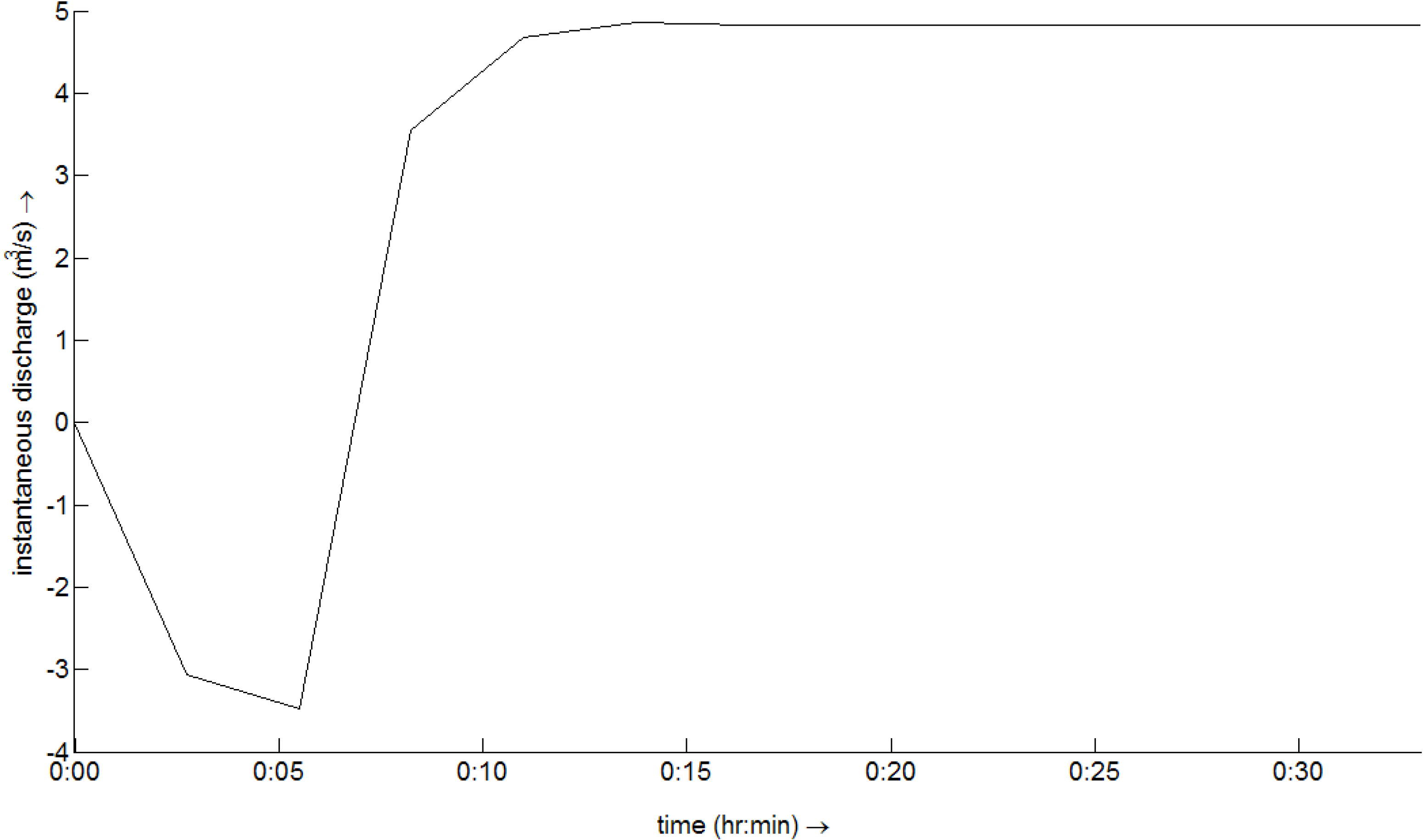
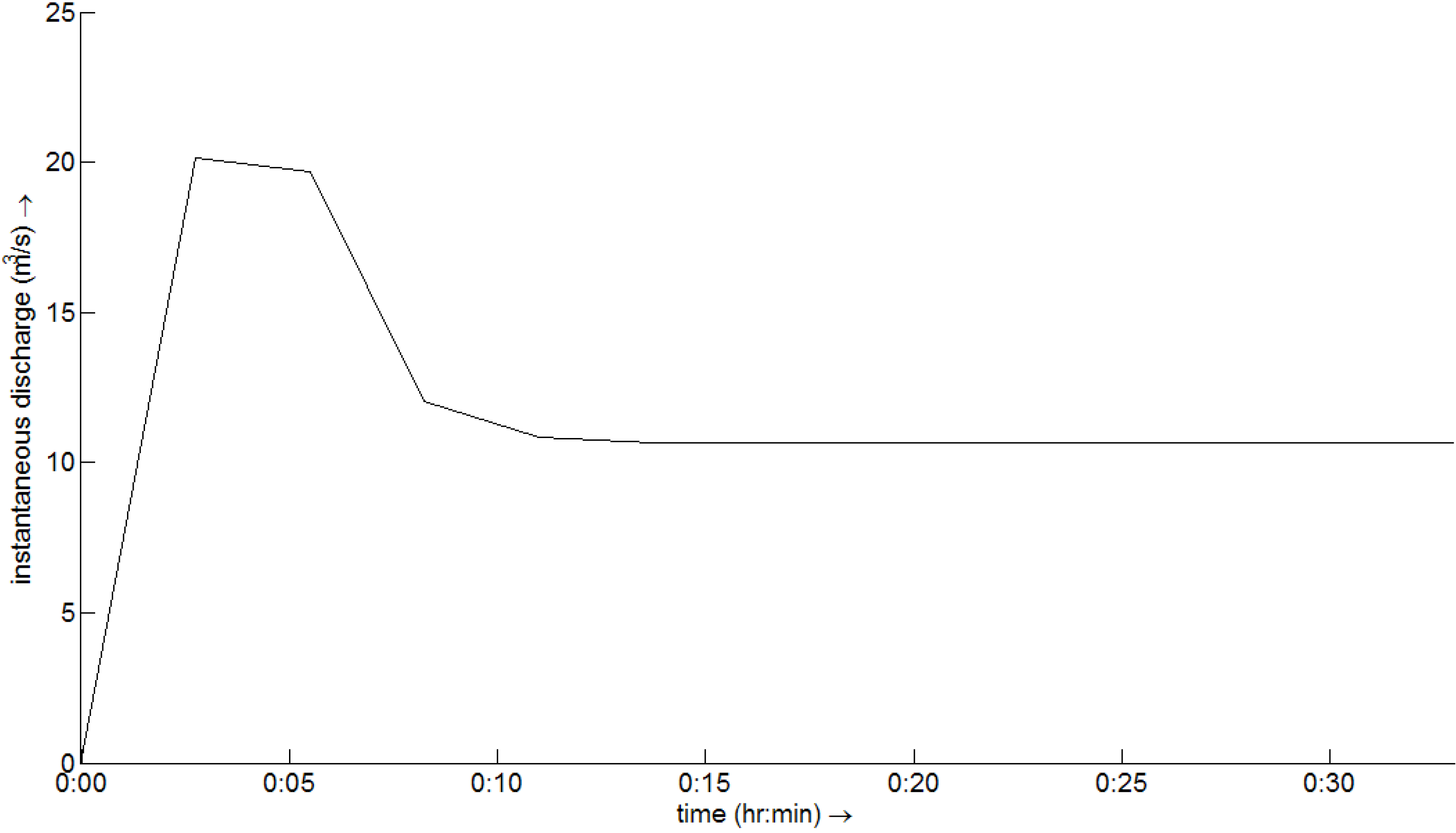
(4) Initial and boundary conditions in agreement with the physics of the flow and numerical accuracy and simplicity were defined. A uniform value of water level was considered for the initial condition. This value was 12.35 m for low discharges (LDS, LDC and LDCV scenarios) and 12.90 m for high discharges (HDS, HDC and HDCV scenarios). The selection of these values corresponds to the selection of upstream boundary conditions, which is described below. Thirty three minutes was found to be much more than the time required to reach the final steady-state condition. This was studied by looking at the variations of the outputs with time at different locations. Figures showing the variations of instantaneous discharges with time, presented in
Section 3, support the approach. Therefore, the following time frame was set for the model to run. Reference date: 12 June 2009; simulation start time: 00hr 00min 00sec, simulation stop time: 00hr 33min 00sec; time step: 0.0001375 day. The selected time step produces stable and accurate results in interaction with the grid size and other numerical and physical parameters, which are introduced in the next items. Among the different types of the boundary conditions supported by Delft3D-FLOW are total discharge boundary condition, discharge per grid cell and water level boundary conditions. In the first step, a total discharge boundary condition was selected for the upstream inflow boundary, and a water level boundary condition was applied at the outflow boundaries along the
E2-F2 and
F2-G2 sections. Unfortunately, in the results, oscillation at the final steady-state depth and discharge values was present. Different measures, such as adjusting the numerical and physical parameters and changing the location of upstream inflow boundaries, were employed to reduce the amplitude of the oscillations. Although moving the location of the upstream inflow section further upstream reduced the amplitude of oscillations at downstream observation points and sections, the oscillations were not completely eliminated. In communications with the model developer, it was explained that the total discharge boundary condition uses the computed water depth just downstream of the boundary to distribute the discharge. Although the model developer explained that this procedure cannot work well in the case of supercritical flows due to the physics of flow, our experience shows that in general, the interaction between depth and discharge adjustment used in the procedure, can result in oscillations that decrease as flow moves downstream. A discharge per cell boundary condition,
i.e., dividing the upstream discharge by the total number of cells, was not used in this study due to the different sizes of the cells. A very effective type of upstream boundary condition was the constant water level boundary condition. This constant depth, with some accepted tolerance (less than 2% of the estimated normal depth of the channel), for low and high discharges was selected based on three sets of data or information: (1) create a depth close to but less than the estimated normal depth in the upstream channel; (2) create a depth close to the depth obtained by taking the moving average of the upstream depths produced by applying the previously described total discharge boundary condition; and (3) create total discharges in agreement with the total discharges reported in
Table 1 for each scenario when adjusting or calibrating horizontal background eddy viscosity, as described later. Considering that the flow after the sill and around and behind the C-Ss was the main focus of this study, no tolerance was accepted for discharge, and continuity was satisfied in all sections including the upstream inflow section. A free overfall condition was observed for the first drop in the numerical results, which agrees with the physical model observations.
Therefore, time series forcing type boundary conditions with the following values were applied to reach the desired final steady-state condition.
For high discharge scenarios:
| Time | Upstream Water Level | Downstream Water Level Along Sections E2-F2 and F2-G2 |
| 00 00 00 | 12.90 m | 12.90 m |
| 00 22 00 | 12.90 m | 6.20 m |
| 00 33 00 | 12.90 m | 6.20 m |
For low discharge scenarios:
| Time | Upstream Water Level | Downstream Water Level Along Sections E2-F2 and F2-G2 |
| 00 00 00 | 12.35 m | 12.35 m |
| 00 22 00 | 12.35 m | 6.10 m |
| 00 33 00 | 12.35 m | 6.10 m |
(5) The physical parameters for the 2D depth-averaged model of Delf3D-FLOW in a one-layer -grid system were selected as follows. A constant gravitational acceleration of 9.81 m/s2 and water density of 1000 kg/m3 were used. The Manning roughness formula with a constant Manning roughness coefficient of 0.013 was selected to represent the bottom roughness in the diversion structure made of concrete. A no-slip condition was applied to the walls. The process of secondary flow, which adds the influence of helical flow to the momentum transport, was ignored. In Delft3D-FFLOW, secondary flow is only displayed for depth-averaged computations using the -grid.
In Delft3D-FLOW, for the Reynolds-averaged Navier-Stokes equations, the Reynolds stresses are modeled using the eddy viscosity concept [
5]. This concept expresses the Reynolds stress component as the product between a flow as well as grid-dependent eddy viscosity coefficient and the corresponding components of the mean rate-of-deformation tensor. The meaning and the order of the eddy viscosity coefficients differ for 2D and 3D, for different horizontal and vertical turbulence length scales and fine or coarse grids. For 3D shallow water flow, the stress tensor is anisotropic. The horizontal eddy viscosity coefficient is much larger than the vertical eddy viscosity. The horizontal viscosity coefficient may be a superposition of three parts.
The horizontal eddy-viscosity is mostly associated with the contribution of horizontal turbulent motions and forcing that are not resolved (sub-grid scale turbulence) either by the horizontal grid or
a priori removed by solving the Reynolds-averaged shallow-water equations. For the latter, Delft3D-FLOW introduces the horizontal eddy-viscosity
and for the former the sub-grid scale (SGS) horizontal eddy-viscosity
. For the latter, Delft3D-FLOW simulates the larger scale horizontal turbulent motions through a methodology called Horizontal Large Eddy Simulation (HLES). The associated horizontal viscosity coefficient
is then computed by a dedicated SGS turbulence model. The 3D part
is referred to as the three-dimensional turbulence, and in 3D simulations it is computed following a 3D-turbulence closure model. The background horizontal viscosity can have user-defined uniform or space varying values. Consequently, in Delft3D-FLOW the horizontal eddy-viscosity coefficient is denoted by [
4]:
It is noted that the background horizontal eddy viscosity represents a series of complicated hydrodynamic phenomena. An overview of different eddy viscosity options in Delft3D-FLOW shows that depending on the selected option, this background horizontal eddy viscosity either contains zero, one or two contributions [
4]. Within the context of the model used in this study and the objectives and availability of data, the option of a 2D-turbulence model with no HLES was used. In this case, conceptually, the background horizontal eddy viscosity contains 2D turbulence effects plus the dispersion coefficient. In simulations with the depth-averaged momentum equations, the redistribution of momentum due to the vertical variation of the horizontal velocity is denoted as dispersion. In this paper, a uniform background horizontal eddy viscosity was considered and manually calibrated. This procedure is described later.
(6) Numerical parameters were specified based on the physics of flow and the recommendations made in the Delft3D-FFLOW user manual. Numerical parameters are mainly related to drying and flooding and some other advanced options for numerical approximations. The Delft3D-FLOW user manual has a detailed description of parameters and practical recommendations for selecting them [
4]. However, some aspects of the model, such as drying and flooding, and numerical methods for the advective terms are briefly introduced here.
Dynamic changes in flow extent are a critical aspect of many environmental flows, including floods, estuarine flows, coastal flows and dam breaks. Such problems all involve a moving shoreline for transient problems or one whose location is not known
a priori in the steady-state case [
6]. Both horizontal and vertical moving boundaries typically require additional algorithms to be incorporated into the code to ensure their correct treatment. A number of such algorithms are available, and the method chosen can have significant consequences for both the computational cost and physical realism of the resulting simulations [
6]. In general, in a numerical model, the process of drying and flooding is represented by removing grid points from the flow domain that become “dry” when the water level falls and by adding grid points that become “wet” when the water level rises. Several drying/flooding schemes are available in Delft3D-FLOW. The detailed description of these numerical schemes is beyond the scope of this paper and can be found in [
4]. However, by default, the water depth in each of the grid cell faces (velocity points) of a computational grid cell is determined to decide if the flow should be blocked by a (temporary) thin dam. If the flow at the four faces of a computational grid cell is blocked, this grid cell is set as dry. However, this does not guarantee the water depth at the grid cell centre (water level point) to be positive definite. Therefore, an additional check can be done on the water depth at the centre [
4]. Drying and flooding can generate small oscillations in the water levels and velocities. These oscillations are small if the grid sizes are small and the bottom has smooth gradients.
For the spatial discretization of the horizontal advection terms, three options are available in Delft3D-FLOW: the cyclic, Waqua, and flooding schemes. The cyclic and Waqua schemes use higher order dissipative approximations of the advective terms, and the time integration is based on the ADI method, which do not impose a time step restriction [
4,
7]. The flooding scheme can be applied for problems that include rapidly varying flows such as hydraulic jumps and bores [
4,
8]. The integration of the advection term is explicit, and the time step is restricted by the Courant number for advection. For this scheme, the accuracy in the numerical approximation of the critical discharge rate for flow with steep bed slopes can be increased by the use of a special approximation (slope limiter) of the total water depth at a velocity point downstream. The limiter function is controlled by the user-defined threshold depth for the critical flow limiter [
4]. In this study, the flooding scheme with a threshold depth for a critical flow limiter of 0.3 m was used in consideration of the physics of the flow and bathymetry of the domain. Reducing the threshold depth to 0.15 m did not affect the results.
As stated by [
4], the standard drying and flooding algorithm in Delft3D-FLOW is efficient and accurate for coastal regions, tidal inlets, estuaries and rivers. Also, in combination with the flooding scheme for advection in the momentum equation, the algorithm is also effective and accurate for rapidly varying flows with large water level gradients, such as the flow system, which was modeled in this study.
A smoothing time of 22 min was selected in the numerical modeling. The smoothing time determines the time interval in which the open boundary conditions are gradually applied, starting at the specified initial condition to the specified open boundary conditions. This smoothing of the boundary conditions prevents the introduction of short wave disturbances into the model.
(7) The uniform background horizontal eddy viscosity
was separately calibrated for low-discharge scenarios LDS and LDC (see
Table 1) and high-discharge scenarios HDS and HDC using the described numerical and physical parameters. The procedure for calibrating
is explained for high-discharge scenarios as example. Depths at three locations were considered for calibration, and these depths for the prototype were calculated by upscaling the measured values at the physical model. The locations were upstream the sill at almost midway between the drop and sill (see
Figure 8), above the sill and in the middle of the corner wall
DE. In total, six depth values were considered in this case, and
in the model was manually changed until a reasonable agreement between the upscaled measured depths and calculated depths and an unbiased error distribution were observed. As described earlier, some tolerance was accepted in imposing the upstream water level boundary condition, but no compromise was made for the discharge. It should be emphasized that the flow pattern downstream the sill, around the corner wall
DE and C-Ss was the main focus of the study and a small tolerance in depth at far upstream section cannot significantly affect the flow in this zone. A similar procedure was used to calibrate
for low-discharge scenarios. The resulting values were
and
m/s
2 for high and low-discharge scenarios, respectively.
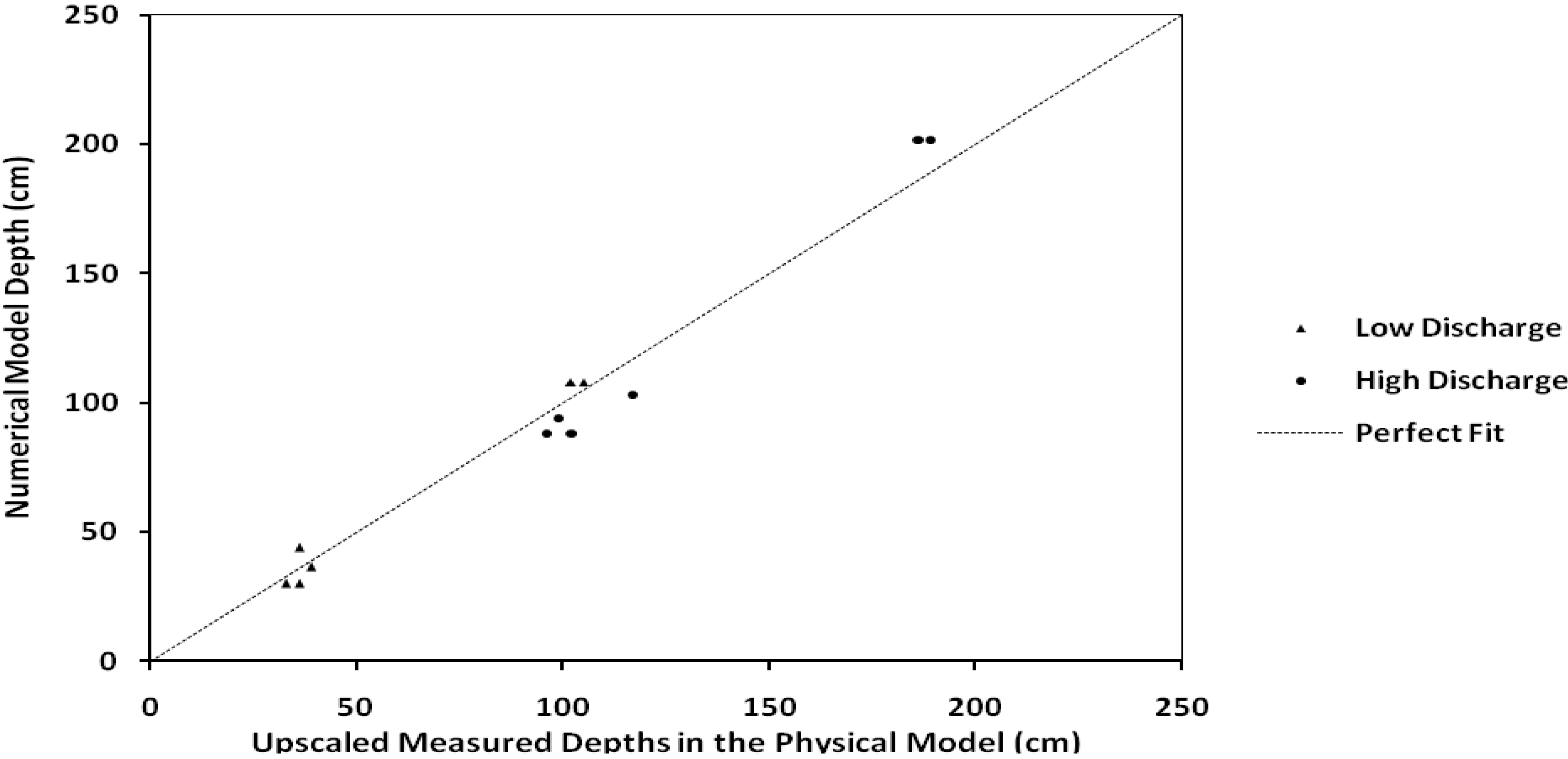
Figure 10 shows simulated
vs. upscaled measured depth values for all three locations under low and high high-discharge scenarios. A mean absolute relative error of about 10% with a maximum absolute relative error of about 22% was observed during the calibration procedure. The reasons for this error can be the upscaled measurement error in the physical model and the simple structure of the numerical model for adequately defining the physical process of the flow system. The stage/ruler used to measure the depths in the physical model was accurate to 1 mm. However, a maximum absolute error of 3 mm can be considered due to the fluctuations in the water surface. Although it is not considered complete turbulence modeling, case studies using a constant eddy viscosity exist in the literature [
9]. It was believed that the adopted numerical and physical values can produce results in agreement with the objectives of the study. The main objective of the study was to generate velocity and depth fields in the areas of interest.
Figure 10.
Upscaled measured depths vs. simulated values after calibration.
Figure 10.
Upscaled measured depths vs. simulated values after calibration.


