
Subgrid Model of Fluid Force Acting on Buildings for Three-Dimensional Flood Inundation Simulations

Department of Civil Engineering, Faculty of Science and Technology, Tokyo University of Science, Chiba 278-8510, Japan
*
Author to whom correspondence should be addressed.
Water 2023, 15(17), 3166; https://doi.org/10.3390/w15173166
Submission received: 6 July 2023
/
Revised: 23 August 2023
/
Accepted: 25 August 2023
/
Published: 4 September 2023
(This article belongs to the Topic Natural Hazards and Disaster Risks Reduction)
Abstract
:In recent years, large-scale heavy rainfall disasters have occurred frequently in several parts of the world. Therefore, a quantitative approach to understanding how buildings are damaged during floods is necessary to develop appropriate flood-resistant technologies. In flood inundation simulations for the quantitative evaluation of a building’s resistance to flooding, a subgrid model is necessary to appropriately evaluate the resistance of buildings smaller than the grid size at a medium grid resolution. In this study, a new subgrid (SG) 3D inundation model is constructed to evaluate the fluid force acting on buildings and assess the damage to individual buildings during flood inundation. The proposed method does not increase the computational load. The model is incorporated into a 2D and 3D hybrid model with high computational efficiency to construct a 3D river and inundation flow model. Its validity and effectiveness are evaluated through comparisons with field observations and the conventional equivalent roughness model. Considering horizontal and vertical velocity distributions, the proposed model showed statistically significant improvements in performance in terms of building loss indices such as velocity and fluid force. These results suggest that the SG model can effectively evaluate the fluid force acting on buildings, including the vertical distribution of flow velocities.
1. Introduction
In recent years, large-scale heavy rainfall disasters have occurred frequently in several parts of the world, such as the disaster concerning the Yangtze River in China in 2020, which caused severe flooding, and millions of people were evacuated [1]. In July 2021, floods hit several river catchments in Germany and Belgium [2,3]. In 2022, floods inundated more than one-third of Pakistan’s land area, destroying 780,000 houses [4], displacing millions of people, and causing shortages of food, shelter, and medical care [5]. In Japan, the heavy rainfall in western Japan in 2018 [6], Typhoon Hagibis in 2019 [7], and heavy rainfall again in July 2020 [8] caused extensive human and building damage. The increase in rainfall and river discharge owing to climate change is a factor that contributes to flood disasters [9,10,11]. For example, Typhoon Hagibis in 2019 increased the total rainfall by 11% owing to climate change effects [12], and its impact on river discharge, water levels, and inundated water volume was also significant [13]. Considering the possibility of further such disasters caused by climate change, it is essential to promote appropriate mitigation and adaptation measures from various perspectives.
Among the types of flood damage, we focused on damage to buildings. When buildings are washed away owing to flood inundation, the direct consequence is human casualties [14]. In addition, the loss or damage to buildings and drift or inundation of household goods cause economic losses [15,16]. Damage to buildings also causes deterioration in the health and sanitation of the residents and damage to social infrastructure facilities such as water, sewage, and electric power systems [17]. These consequences significantly impact the post-disaster recovery status [18]. However, general building design considers only earthquakes, wind, and fire as external forces; flood inundation flows are not considered [19,20,21,22]. Land use regulations and town development are certain soft measures that can be adopted to mitigate damage to buildings, but the realization of these measures requires significant effort, time, and cost [23,24]. Therefore, there is an urgent need to quantitatively understand how buildings are damaged during flooding and develop flood-resistant technologies for buildings. In addition, the mitigation measures adopted for building damage caused by inundation could be a significant step toward adapting to climate change.
Flood inundation simulations are useful for quantitatively understanding and evaluating the strength of buildings against inundation flows. Several flood inundation models that incorporate buildings have been proposed so far. For example, Schubert and Sanders [25] classified four types of models according to the treatment of buildings: building resistance (BR), building block (BB), building hole (BH), and building porosity (BP) methods. They compared the methods in terms of their accuracy, calculation time, and setup time. The BR method assigns large resistance parameters (mainly equivalent roughness coefficients) to the computational grid containing the buildings [26,27]; the BB method assigns roof height to the ground level of the computational grid containing the buildings [28,29]; and the BH method incorporates a slip wall boundary condition along the building wall [30,31]. In addition to the resistance of the building, the BP method considers the percentage of nonbuilding area (porosity) from the building area in the grid [32,33]. Schubert and Sanders [25] obtained the following results based on the analysis of an unstructured grid using the four methods: The BR method demonstrates low calculation accuracy. The BB and BH methods involve high computational loads, are computationally demanding, and require a large amount of effort to set up. The BP method provides a good balance between accuracy and computational load. These results obtained for unstructured grids are expected to be applicable to structured grids as well. However, for validation, only the inundation flow behavior, such as the reproducibility of the horizontal velocity distribution through the road network, was considered, and the fluid force acting on the buildings or the extent of damage was not considered.
To assess building damage caused by flood inundation, it is necessary to evaluate the fluid force acting on each building, determine the damage—such as the loss or destruction of each building based on the fluid force—and feed this information back to the flood inundation model. To correctly determine the fluid force acting on a building, a sufficiently fine grid resolution (<1 m) is required to calculate the surface distribution of the pressure and shear stress around the building. Among the four models, the BB and BH models adopt this approach and are referred to as “microscopic models” [34,35,36]. In contrast, for wide-area inundation analyses, the grid resolution is coarser (for example, >30–50 m) and “macroscopic models” are used, which involve several buildings [37,38,39]. The BR and BP models are macroscopic models. However, with the recent remarkable improvements in computational power and resources, inundation analyses with fine grid resolutions have been conducted for wide areas, and several analyses with medium grid resolution, where the grid resolution is of the order of 10 m, have also been conducted [40,41,42]. However, because the grid resolution is of the same order as the building size, it is based on the BR and BP models, which have the following drawbacks: the fluid force on each building is not properly evaluated, buildings exist over several computational grids, and the calculation becomes unstable when the entire grid is covered by buildings, that is, when porosity is zero. To address these issues and evaluate the fluid force acting on individual buildings, a subgrid (SG) model that can appropriately evaluate the location and height of buildings below the grid size and their resistance forces is required; however, no appropriate SG model is currently available. In particular, a SG model based on a three-dimensional (3D) flow model that considers the 3D structure of a building is required to study the effects of embankments [43] and pilotis systems [44,45]. However, no corresponding SG models are available; even 3D flow models are not available for inundation analysis.
The objective of this study is to develop a 3D inundation model by introducing a new subgrid model for evaluating the fluid force acting on buildings to assess the damage to individual buildings during flood inundation without increasing the computational load. The SG model is based on the BR model and reflects the building effects only in the momentum equations. The porosity of buildings is not treated here but will be the subject of future studies. The fundamental structure of the model and fundamental equation system are presented. As a case study of the application of the model, a reproduction analysis of the river and inundation flows in the Kuma River, Japan, caused by the heavy rainfall in July 2020 [8] was conducted to evaluate its validity and effectiveness through comparisons with field observations and the conventional equivalent roughness model, which is commonly used as the BR method. The relationship between hydraulic quantities, such as the horizontal and vertical flow patterns, and the fluid force obtained from the analysis was also verified.
2. Materials and Methods
2.1. Fundamental Concept of SG Model for Building Fluid Force
In this study, we constructed a SG model for the fluid force acting on buildings, which can be introduced into a 3D inundation analysis model to appropriately evaluate the fluid force on each building of the grid size or smaller. The fundamental concept of the SG model is illustrated in Figure 1. When a medium grid resolution is used based on building data (location, horizontal shape, height, and so on), it is assumed that multiple buildings are included in the computational grid or that a single building is located across multiple grids. In addition, the height of each building varies, such as one- or two-story buildings, and the presence of buildings changes significantly in the vertical direction when the pilotis system is considered (Figure 1a). To investigate the effect of these factors, Step 1 is to divide each building into horizontal and vertical directions in each computational grid and calculate the volume occupancy α in the grid relative to the volume of the entire building (Figure 1b). In Step 2, the flow velocity at each grid point obtained from the numerical analysis is interpolated to the location of the building center to calculate the fluid forces acting on each building (Figure 1c). Finally, in Step 3, the fluid forces obtained for each building are allocated to each grid using the volume occupancy α in each grid. The fluid forces from multiple buildings are summed in each grid, and the result is reflected in the momentum equations of the fluid (Figure 1d).
The advantages of the proposed SG model based on the above concepts are that it can appropriately reflect the 3D information (shape, height, and so on) of the building below the grid size to the extent available and calculate the fluid forces acting on each building individually. Therefore, the model can express the fluid resistance of buildings in more detail, considering the 3D information of the building, when compared with the BR method, which only describes the building information through resistance parameters such as the roughness coefficient. The computational load is lower than those of the BB and BH methods, and less effort is required to set up the input conditions because the grid size is not limited by the building, and there is no need to represent the building shape in grid form. Thus, the model can accurately evaluate the fluid forces acting on buildings, including those in the vertical direction, while maintaining computational efficiency. Furthermore, because the model evaluates the fluid forces on each building individually, it is easy to predict the loss of each building during a flood after the building loss conditions are established. In densely built areas, the loss of a building upstream of a flooded area is expected to significantly increase the fluid forces on buildings downstream of the lost building and increase the risk of downstream building loss. The proposed SG model can be applied to such a situation, and it can be a useful tool to consider changes in fluid forces caused by building loss if the conditions for determining building loss are developed.
As illustrated in Figure 2, inverse distance weighting (IDW, [46]), which is a common spatial interpolation method incorporated into GIS software, was adopted as the interpolation method for the flow velocity data used to calculate the fluid force, which is the key to this model. In particular, because a staggered grid was used for the flow velocity definition position in the flow analysis described below, four velocity definition points surrounding the building center were calculated in each direction (represented by blue and red boxes in Figure 2) and interpolated through IDW (Figure 2). In addition, the spatial pattern of the flow velocity within the grid varied significantly based on the arrangement and porosity of buildings within the grid. It is necessary to consider this when interpolating the spatial pattern of the flow velocity within the grid, which will be a subject for future work.
2.2. Fundamental Equations of SG Model
A hybrid 2D–3D flow (Hy2-3D) model was used as the 3D flow model to introduce the SG model [47,48,49]. This model enables wide-area analyses while considering computational efficiency. In the Hy2-3D model, horizontal 2D and 3D flow calculations are performed in parallel, with the 2D calculation performed at every time step and the 3D calculation performed once every several to several dozen steps (Figure 3a). The Hy2-3D model is characterized by the fact that the time interval of the 3D calculation can be set without the impact of the Courant–Friedrichs–Lewy (CFL) condition. This enables a significant reduction in the computational load, which is unique to 3D calculations. In particular, the time interval for 3D calculations Δt3D is divided into Δt3D1 and Δt3D2, and within Δt3D1, horizontal 2D and 3D calculations are performed, and the results of both calculations are exchanged. However, within Δt3D2, only horizontal 2D calculations are performed without 3D calculations, and the results of the 3D calculations performed within Δt3D1 are continuously reflected in the horizontal 2D calculations. Thus, Δt3D2, which does not perform 3D calculations, is not restricted by the CFL condition and Δt3D2 can be set to a large value, resulting in improved calculation efficiency. It should be noted that the computation time interval Δt2D for a horizontal 2D analysis does not necessarily have to match that of Δt3D1 (Figure 3b). To reflect the results of the 3D calculation on the horizontal 2D calculation, the difference between the depth-averaged terms in 3D equations of motion and each term in the horizontal 2D equations of motion is calculated as a correction term at Δt3D1. The correction term is incorporated in the horizontal 2D equations of motion. In contrast, to reflect the results of a horizontal 2D calculation in a 3D calculation, the depth-averaged velocity in the previous 3D calculation is replaced by the result of the horizontal 2D calculation. In other words, the vertical velocity distribution in the previous 3D calculation is retained, but the depth-averaged velocity is updated.
The SG model was introduced based on the concept of the Hy2-3D model. First, we describe the fundamental equations for the 3D and horizontal 2D calculations in the Hy2-3D model, which adopts the Cartesian curvilinear coordinate system (in the s, n directions) in the horizontal direction and the σ coordinate system (σ = (z − η) / D, D: depth, η: water level) as its coordinate systems, which are boundary-fitted coordinate systems [47]. With river and inundation flow analyses being the focus, 3D calculations based on these coordinate systems consider the fluid forces on buildings and bridge girders obtained by the SG model using the fundamental equations [47] based on the hydrostatic pressure approximation. The continuity equation for the 3D field is expressed by Equation (1), and the momentum equations in the s and n directions are expressed by Equations (2) and (3), respectively.
where us, un, and w* are the velocities in the s, n, and σ directions, respectively; R is the radius of curvature in the s coordinate; N = n/R; g is the acceleration owing to gravity; is the density of water; AH and AV are the horizontal and vertical eddy viscosity coefficients, respectively; and Fbs, Fbn and Fgs, Fgn are the building and bridge girder fluid forces per unit mass in the s and n directions, respectively. In the Hy2-3D model, the vertical eddy viscosity coefficient AV is expressed by the zero-equation model, which is one of the turbulence models, and the horizontal eddy viscosity coefficient AH is expressed in a simple form proportional to AV:
where is Kalman’s constant (=0.40), is the friction velocity, is the height from the bottom, and is constant (=10) [47]. The friction velocity is expressed by the results of the horizontal 2D calculations described in Equation (15).
In formulating the building fluid forces Fbs and Fbn obtained using the SG model, the fluid force is obtained for each building and distributed to each grid according to the fraction α occupied by the building, as depicted in Figure 1. In particular, if the number of buildings in each grid is Mmax, the fluid force in the s direction acting on building m (=1 − Mmax) is fbs(m), and the volume of the building with the volume Vb(m) in the grid is Vb′(m), and the fluid force distributed in this grid is fbs(m)Vb′(m)/Vb(m). When deriving the momentum equations, both sides are divided by the mass of the control volume (, : grid volume), so that Fbs is expressed as follows:
where the volume occupancy of building m in the target grid, α(m), is the ratio of Vb′(m) to the grid volume ΔV. Similarly, if the fluid force in the n direction acting on building m is fbn(m), Fbn is expressed as follows:
The fluid forces fbs, fbn in the s, n directions acting on individual buildings are expressed using the general drag formula as follows:
where B is the average building width, h′ is the inundation height of the building, the product of the two represents the projected area of the building, CDb is the drag coefficient of the building, and are the velocities in the s, n directions interpolated at the building center. The available building information includes the building width and building plane area Ab. However, because it is complicated to calculate the building width perpendicular to the flow direction data obtained from this calculation, we assume that the building is square and obtain the building mean width B using the following equation:
In Equation (10), the building width for evaluating the projected area is simply calculated as suggested by Imai et al. [50]. We need to improve the description of building width in future work.
The inundated building height h′ is chosen to be the smaller of the building height h and water depth D, as given by the following equation:
The building drag coefficient CDb in Equations (8) and (9) are set to 1.2 based on the experimental results reported by Kuwahara [51]. The fluid forces on the bridge, Fgs and Fgn, are also expressed in the same way as the fluid forces on the building but are omitted here.
Next, the continuity equation for the horizontal 2D field in the Hy2-3D model and the equations of motion in the s and n directions are expressed by Equations (12)–(14), where Us and Un are the depth-averaged velocities in the s and n directions, respectively:
where AH2D is the depth-averaged horizontal eddy viscosity coefficient, Cf is the bottom friction coefficient, and Gs and Gn are correction terms in the s and n directions, respectively, reflecting the results of the 3D calculation in the horizontal 2D calculation. The bottom friction coefficient Cf and friction velocity in Equation (4) are expressed as follows:
where n represents Manning’s roughness coefficient. In the momentum equations for a horizontal 2D field (Equations (13) and (14)), as is generally the case (for example, Wu [52]), the unsteady and advection terms are considered on the left-hand side, and the water surface gradient, diffusion, and bottom friction terms are considered on the right-hand side. When compared with the momentum equations for a 3D field (Equations (2) and (3)), neither the building and bridge girder resistance terms nor the three-dimensionality of the flow field in the advection and diffusion terms are considered. The correction terms Gs and Gn used to account for these effects are expressed by the following equations, which represent the differences between the depth-averaged 3D and horizontal 2D results:
The vertical integration of the vertical diffusion terms (Equations (2) and (3)) on the right-hand side of the momentum equations for a 3D field yields the shear stress (Reynolds stress) on the bottom and water surfaces. At the water surface, the shear stress is zero owing to the slip condition, and the frictional stress at the bottom is consistent with the bottom friction term (Equations (13) and (14)) on the right-hand side of the horizontal 2D momentum equations. Therefore, the correction terms of Gs and Gn do not include a vertical diffusion term. For details on the calculation procedure for the Hy2-3D model, please refer to Nihei et al. [47]. Additionally, it is noted that the density of the fluid does not vary, and the proposed model does not apply to saline water.
2.3. Study Site
The Kuma River, the site of this study, flows through Kumamoto Prefecture in the Kyushu region of Japan and has a channel length of 115 km, a basin area of 1880 km2, and a population of approximately 140,000 within the basin. It is a first-class river managed by the national government [53]. As depicted in the elevation contour (Figure 4a), the Kuma River Basin is surrounded by steep mountains, and the river is one of the three most rapid rivers in Japan. The topographical features of the Kuma River Basin include the Yatsushiro Plain in the lower reaches (0–10 km point (kp)), a narrow mountain channel in the middle reaches (10–52 kp), and the Kuma Basin in the upper reaches (52 kp). The entrance to the middle reaches becomes constricted during floods, and the Hitoyoshi urban area, located upstream of the constricted area, tends to become vulnerable to inundation damage [53].
In 2020, a training rainband covered the entire Kuma River basin from 3 July to 4 July, causing heavy rainfall; the associated flooding led to extensive human and property damage [54]. Referring to Figure 5a, the basin-averaged hourly precipitation exceeded 40 mm from early morning on 4 July, and the cumulative rainfall reached approximately 400 mm, which was much higher than the planed rainfall. The water level of the Kuma River started to increase significantly in the early morning of 4 July, peaking at 10:00 a.m. on the same day (Figure 5a). The peak water level significantly exceeded the height of the levee, leading to widespread overflow flooding. Because the Kuma River is surrounded by mountainous terrain, the river and inundation flows were integrated and flowed downward together. The flooding caused tremendous water depths and high velocities in the inundated areas, and the human casualties in the basin reached as high as 50 [8].
Ogata et al. investigated the flood inundation and building damage caused by the torrential rainfall immediately after the disaster [55]. All the buildings within the inundation area were visually classified as “loss”, “no loss with inundation”, or “without inundation”. It was found that the maximum depth of inundation exceeded 7 m and that the lost houses were concentrated along the river (Figure S1). The accuracy of this analysis was verified by comparing these observations with the results of the inundation analysis.
Significant damage was caused to buildings in the Chaya district, located at 53 kp on the Kuma River (Figure 4b). In this area, the maximum depth of flooding reached 7.4 m, and 32 of the 70 buildings were lost. Figure S2a presents a building damage map with an aerial photograph in the background. Although several buildings were lost on the eastern side (far from the river) of Prefectural Road 325, several survived on the western side (near the river). As depicted in Figure S2b, the building located at the upstream end of the surviving buildings is a pilotis-style building in which the first floor dodges the flood flow, making it resistant to the flooding. This implies that the strength of the upstream building may have prevented damage to the buildings behind it. This case must be clarified when considering urban development that is resistant to flood damage from the viewpoint of building standards and layouts.
2.4. Computational Conditions
Using the proposed model, we conducted an integrated analysis of river and inundation flows in the Kuma River and the surrounding inundation area. The computational domain was 51.8–68.6 kp of the Kuma River and its surrounding flooded area, as depicted in Figure 4b (computational domain size: 15,340 m × 1510 m). The grid spacings were approximately 20 and 10 m in the streamwise (s) and spanwise (n) directions, respectively. In the vertical direction, the water depth was divided into 10 layers using the σ coordinate system. The topographic data were interpolated for the streamwise direction in the river channel using cross-sectional survey data (provided by the Ministry of Land, Infrastructure, Transport, and Tourism) and in the flooded area using a digital elevation model (Geospatial Information Authority of Japan, https://fgd.gsi.go.jp/download/menu.php (accessed on 2 December 2022)) with a resolution of 5 m. For the 3D calculations, = 0.05 s, = 10.0 s, and the time interval ratio = 200 was fixed as the computation time interval. For the horizontal 2D calculations, was determined for computational efficiency from 0.125–0.500 s to a maximum Courant number below 0.2, and the time-interval ratio for the 2D and 3D calculations, , was set to 20–80. The upper limit of the Courant number was pre-decided in order to maintain the numerical stability since the numerical solution did not converge when the Courant number was 0.3 in the preliminary calculations. The calculation period was from 1:00 a.m. to 5:00 p.m. on 4 July 2020. As boundary conditions, the upstream boundary discharges of the Kuma River and 11 major tributaries (for example, Kawabe River, Figure 4b) were obtained from the runoff calculation results [49] using the rainfall–runoff–inundation model [56] (Figure 5b). The water level at the downstream boundary of the computational domain was set using the results of a preliminarily performed 1D unsteady flow calculation (Figure 5b). At the upstream and downstream boundaries, other variables were subjected to open boundary conditions, with the gradient of the variables in the streamwise direction being zero. A wall law and slip condition were given at the riverbed and water surface, respectively. A no-slip condition is added at the side boundaries of the computational domain. To trace wet/dry fronts while maintaining high numerical stability, the flow velocity was determined by solving a simplified equation of motion, which included only a water surface gradient term and a bottom friction term. Manning’s roughness coefficient n was set to 0.030 m−1/3 s in the 58–64 kp section of the river channel and to 0.035 m−1/3 s in the other sections. To verify the fundamental performance and effectiveness of the SG model, we compared the case of the SG model (Case 1) with the case where the roughness coefficient had an equivalent roughness value in the flooded area, as in the BR model (Case 2) as well as the case where the roughness coefficient was constant (Case 3-1, n = 0.06 m−1/3 s; Case 3-2, n = 0.03 m−1/3 s). The following equation was used for the equivalent roughness n in Case 2 [50]:
where n0 is the roughness coefficient on the ground (=0.03 m−1/3 s) and θ is the occupancy of the building in the grid. In Case 1, the roughness coefficient was required to evaluate the bottom friction in the flooded area and was set uniformly to n = 0.030 m−1/3 s.
The computational domain includes 10,161 buildings. The ArcGIS data includes the building plane form (width and area), with building height given in increments of 3 m over 6 m. Because these data do not cover the downstream area, the building data from OpenStreetMap (OpenStreetMap Foundation, https://www.openstreetmap.org/ (accessed on 17 February 2023)) were used for the missing areas. The OSM data contain information only on the planar geometry; they do not contain height information. Therefore, the buildings in the OSM data are assumed to be uniformly 6 m high (equivalent to a two-story building). The building floors in the computed area were mostly first and second floors, with the exception of certain areas. Therefore, the number of building floors and the presence or absence of pilotis were visually determined using Google Street View only in Chaya village (Figure 4a), where the damage to buildings was significant, and used as building data for this analysis. The building data were processed using GIS software to calculate the building plane area Ab and the location of the building center. A histogram of building width B (Figure S3) indicated that most of the building widths measured between 8 and 12 m, which was approximately the same as the grid resolution. Some buildings were smaller than the grid resolution, whereas others spanned several grids. In this analysis, the CPU time was approximately 12 h when we used an Intel(R) Xeon(R) W-2245 CPU @ 3.90GHz with RAM of 64.0 GB computer for numerical analysis.
3. Results and Discussion
3.1. Validation of Hy2-3D Model
To validate the results of the flood inundation flow analysis using the Hy2-3D model, a comparison of the observed [55] and calculated values for the longitudinal distribution of water levels along the Kuma River is presented in Figure 6. Here, because the differences among the four cases set up as building models were small, the calculations for the temporal variation of the longitudinal distributions of the water level (Figure 6a) and peak water level (Figure 6b) indicate those in only the SG model (Case 1). For the peak water level, the differences in the longitudinal distributions among Case 1 and the other three cases (Cases 2, 3-1, 3-2) are displayed (Figure 6c). First, the results of the present analysis (Case 1) indicate that the temporal variation in the longitudinal distribution of the water level accurately captures the observed data and that the peak water level is also generally reproduced. The difference between Case 1 and the other three cases with respect to the peak water level is the smallest in absolute value (0.09 m at maximum) with the Case 2 equivalent roughness model. In contrast, even for Cases 3-1 (n = 0.06 m−1/3 s) and 3-2 (n = 0.03 m−1/3 s) with constant roughness coefficients, the maximum absolute values of the peak water-level difference were 0.15 and 0.45 m, respectively. This result indicates that even if n is kept constant, the results do not change significantly from those of the equivalent roughness model if an appropriate value (Case 3-1 in this case) is used. In Case 3-2, n = 0.03 m−1/3 s, the peak water level difference in the river is roughly within 0.25 m except at 61 kp, and the impact of the resistance evaluation of the flooded area on the river water level is very small because the river and inundation flows are combined. It is concluded that the accuracy of the Hy2-3D model is generally good, regardless of the building resistance model used.
Next, Figure 7 presents a comparison of the observed and calculated values (Case 1) for the water level hydrograph. Six water level observation stations in the computational domain were covered, from upstream: Ichibu (68.6 kp), Hitoyoshi (62.2 kp), Ohashi (61.5 kp), Nishizebashi (59.4 kp), Gogan (57.4 kp), and Watari (52.7 kp). Note that some of the measured data are missing at the three downstream sites owing to the large flood magnitude. At Ichibu station, which is the upstream boundary of the computation domain, although the discharge was considered as a boundary condition instead of the water level, the root mean square error (RMSE) and the root relative mean square error (RRMSE) of the difference between the observed and calculated water levels during the flood were 0.44 m and 9.3%, respectively, which are generally good for the calculation accuracy of the analysis results. At the Hitoyoshi and Ohashi sites, for which there were no missing data, the calculated and observed water levels generally agreed during the rising stage; however, the difference between the two sites was larger during the falling stage. Among the three downstream stations, for which data were missing, the accuracy of the Gogan site was the highest (RMSE = 0.33 m and RRMSE = 5.3%); however, at the Nishizebahi and Watari sites, there was a discrepancy between the calculated and observed water levels, even during the rising stage, when the observed data were available. As described previously, the calculated and observed water levels differed at each water-level station. This result appears to be attributable to the methods used to set the roughness coefficient n in the river channel and discharge of the tributary river as the inflow condition. The RMSE and RRMSE of the calculated results in Case 1 ranged from 0.33 to 1.09 m and from 5.3 to 17.7%, respectively, demonstrating that the results of this analysis were generally good. The RMSEs and RRMSEs of all the six sites in the other cases were the same as those in Case 1, with a maximum difference of only 0.08 m and 1.9%, respectively (Figure S4).
To verify the accuracy of the calculations in the Hy2-3D model quantitatively, the scatter plots of the calculated and observed results at the peak water level and depth are presented in Figure 8. The high water mark levels and depths obtained from the field observations reported by Ogata et al. [55] (165 data points) are presented along with the calculated results for Case 1.
For the peak water level (Figure 8a), the RMSE of the difference between the observed and calculated values was 0.38 m, the slope of the regression line between them was 1.021, and R2 = 0.990, indicating that the calculated values were generally in good agreement with the observed values. Similarly, for the peak water depth, the RMSE of the difference between the observed and calculated values was 0.45 m, and the slope of the regression line was 0.930 and R2 = 0.937, indicating that the calculated values were in good agreement with the observed values. The RMSE of the peak water depth was larger than that of the peak water level because it reflected the spatial variation in the ground height data.
Table 1 summarizes the RMSEs of the differences between the calculated and observed values of the peak water level and depth, slope of the regression line, and R2 for all cases. The RMSEs in Cases 2 and 3-1 were similar to those in Case 1, and the slope of the regression line was almost unity. In Case 3-2, the RMSE was larger than those in the other three cases for both the peak water level and depth. A significance test between Case 1 and the other three cases for the difference between the calculated results and the observed data indicated a statistically significant difference (p < 0.05) only in Case 3-2 but not in Case 2 or 3-1. Thus, it is quantitatively clear that there is no statistically significant difference between Case 1 of the SG model, Case 2 of the equivalent roughness model, and Case 3-1 of the appropriate constant roughness coefficient (=0.06 m−1/3 s) with respect to the reproducibility of water level and depth in the river and inundation flow analysis. It is clear that the impact of the building resistance evaluation model is small. The validity of the Hy2-3D model, which is the basis of the analysis, was also verified. The high reproducibility of the water level and depth distribution in the Hy2-3D model, despite the simple and almost uncalibrated setting of the roughness coefficient in the river channel, may be attributed to the good reproduction of the complex flow distribution and the appropriate introduction of resistances, such as bridge girders.
3.2. Horizontal Map of Velocity Distribution
To compare and validate the results of the velocity field analyses, which are significant for the assessment of building damage, horizontal velocity contours are presented in Figure 9a for the Hitoyoshi city area (59.0–61.2 kp), where the inundated area is large and urbanization is in progress. The depth-averaged velocity contours for all four cases are shown for 10:00 a.m. on 4 July, when the water level and velocity peaked. A residential map displaying the locations and sizes of the roads and buildings is used as a background image for the contours and is superimposed on the velocity contours. In Cases 3-1 and 3-2, there is a wide area of high velocity in the inundated area. This tendency is more pronounced in Case 3-2, in which the roughness coefficient is small. However, in Cases 1 and 2, there are generally low flow velocities in the inundated area, reflecting the fluid resistance caused by the buildings. High flow velocities can be observed locally, and this tendency is more pronounced in Case 1.
To evaluate this result in detail, the horizontal velocity distribution on the A-A′ cross section indicated in Figure 9a is depicted in Figure 9b. Again, as in Figure 9a, the calculations for all cases on 4 July, 10:00 a.m. are indicated, and the building location, water level, and ground elevation are also depicted. First, Case 3-2 (with n = 0.03 m−1/3 s) indicates a high flow velocity and low water depth across the entire cross-section. In Case 3-1 (with n = 0.06 m−1/3 s), the velocity levels are similar to those in Cases 1 and 2, but the fluctuations in the velocity distribution are smaller, and there is no indication of a decrease in velocity near the buildings or an increase in the velocity on the road without buildings. However, in Cases 1 and 2, the contrast in velocity fluctuation was larger than those in Cases 3-1 and 3-2, with lower velocities in the building area and higher velocities on the road. However, a closer look reveals that the flow velocity in Case 1 is higher than that in Case 2 on the road and in areas without buildings and that the flow velocity in the grid where buildings exist is often larger for Case 1 than for Case 2. The RMS of the flow velocity in the A-A′ cross section is 1.20 and 1.16 m for Cases 1 and 2, respectively, indicating that the fluctuation of flow velocity for Case 1 is larger than that for Case 2. This reflects the fact that the difference in flow velocity between the grids with and without buildings is larger in Case 1, as described above. Case 1, which uses the SG model, indicates low velocities on the building grid and high velocities on the grid without buildings, for example, on the road, owing to low resistance, suggesting that the SG model adequately evaluates the fluid force acting on buildings. The values of velocity on the grid with buildings were in the order Case 1 > Case 2 because the high velocities on the nonbuilding grid, such as roads, diffused horizontally and caused the velocities on the building grid to be relatively large. In addition, because equivalent roughness is used in Case 2, the roughness coefficient affects the vertical and horizontal eddy viscosity coefficients (Equations (4) and (5)) as well as the bottom friction force in this model. Therefore, the spatial variation in the velocity distribution is expected to be less sharp than that of the SG model (Case 1) because of the effect of the increased roughness on the area around the building grid. It is also noted that the water level decreased and increased near the lateral distance of 200–250 m and 250–400 m, respectively. This is because the higher ground elevation in the lateral distance of 200–250 m results in lower water levels due to high drag and inadequate water supply from the upstream side.
3.3. Vertical Distribution of Streamwise Velocity
To compare the changes in the vertical distribution of the flow velocity owing to the presence or absence of buildings among the different cases, the vertical distributions of the horizontal flow velocity at the feature points in Chaya District in Cases 1 and 2 are depicted in Figure 10. We extracted the vertical distributions of the flow velocities at four calculation grids (Figure 10a), which included Stn A: no buildings, Stn B: one-story buildings, Stn C: two-story buildings, and Stn D: pilotis style buildings in which the first floor with 2 m height dodges the flood flow, as the feature points in Chaya District. Because the flood flow in Chaya District was dominated by the main flow direction (s), the velocity in the s direction is depicted. The results at 11:30 a.m. on 4 July 2020, which was the peak time of the downstream water level, are presented. Focusing on Case 1, the vertical distribution of the flow velocity at Stn A (no buildings) has a typical logarithmic distribution. At Stn B (one-story buildings), the distribution of the flow velocity was small below the height of the first floor (3 m) and had an inflection point at approximately 3 m. Above that, the velocity increased. At Stn C (two-story building), the inflection point of the flow velocity appeared at approximately 6 m, which corresponded to the height of the second floor, and the flow velocity was small below 6 m. Thus, when the water depth exceeded the building height, as in Stn B and Stn C, the flow velocity distribution inside and outside the canopy layer appeared to have an inflection point near the building height [57], leading to a vertical velocity distribution different from a logarithmic distribution. At Stn D (pilotis), the maximum velocity appeared at a height of 1.6 m; the velocity was high below the height of 2.5 m and low above that height, corresponding to the building type.
In Case 2, Stn A, where no buildings exist, exhibits a general logarithmic distribution, as in Case 1, whereas Stn B, C, and D, where buildings exist, exhibit the same vertical velocity distribution, with no difference based on the building structure. One of the most significant features was that the velocity near the bottom was negative at Stn B, C, and D. The roughness coefficient calculated using the equivalent roughness model in Case 2 reached a maximum of 0.3 m−1/3 s, which is a significantly large value (Figure 10b). This results in a significant roughness height ks, which is considered responsible for the negative velocity near the bottom. This is similar to the zero-plane displacement in atmospheric turbulence fields over urban canopies [58]. These results indicate that the equivalent roughness model has limitations in accurately reproducing 3D flow velocity distributions around buildings with large roughness coefficients. It was also suggested that the SG model can reproduce the vertical velocity distribution based on the vertical structure of a building.
3.4. Hydraulic Factors of Building Damage
To understand the characteristics of the building loss indices obtained using the SG model, the correlation plots of the calculated results for Cases 1 and 2 for the lost buildings (160 buildings) are presented in Figure 11. The maximum values of water depth h, depth-averaged velocity v, unit-width discharge q, moment qh, and fluid force F were selected as the building loss indices. It should be noted that the time of the maximum value of each index does not coincide. For each index, the approximate linear equation and the coefficient of determination R2 are also shown. The p-values obtained by the t-test are also depicted to check for significant differences between the results of Cases 1 and 2. In Case 1, the fluid force F is obtained directly for each building, but not in Case 2. Therefore, the same method used in Case 1 was applied to calculate F in Case 2. The water depth h was plotted on y = x, and there was no significant difference between the cases (p > 0.10). This is because, as depicted in Section 3.1., the present inundation pattern is a flood in which the river and inundation flows are combined, and the water level of the river largely determines the water level in the inundated area. The variation in the flow velocity between the cases increased, particularly when the velocity exceeded 2.0 m/s. It was confirmed that the velocity in Case 1 was generally larger than that in Case 2. There was a statistically significant difference between Cases 1 and 2 (p < 0.10) at the 10% significance level. For the unit width discharge q and moment qh, the variation increased with v, and a significant difference was confirmed between the two cases (p < 0.05). Furthermore, for the fluid force F, the variation between the two cases was larger than that for the flow velocity, with the slope of the approximate line reaching 1.07. Because fluid force F is the product of h and v squared, the effect of the flow velocity was more pronounced. The difference between the two cases was significant at the 10% level (p < 0.10). The fluid force is a flood index that determines building damage, and the fact that this assessment differs significantly between the SG model and the conventional equivalent roughness model suggests that the assessment of building damage differs significantly depending on the difference in the models.
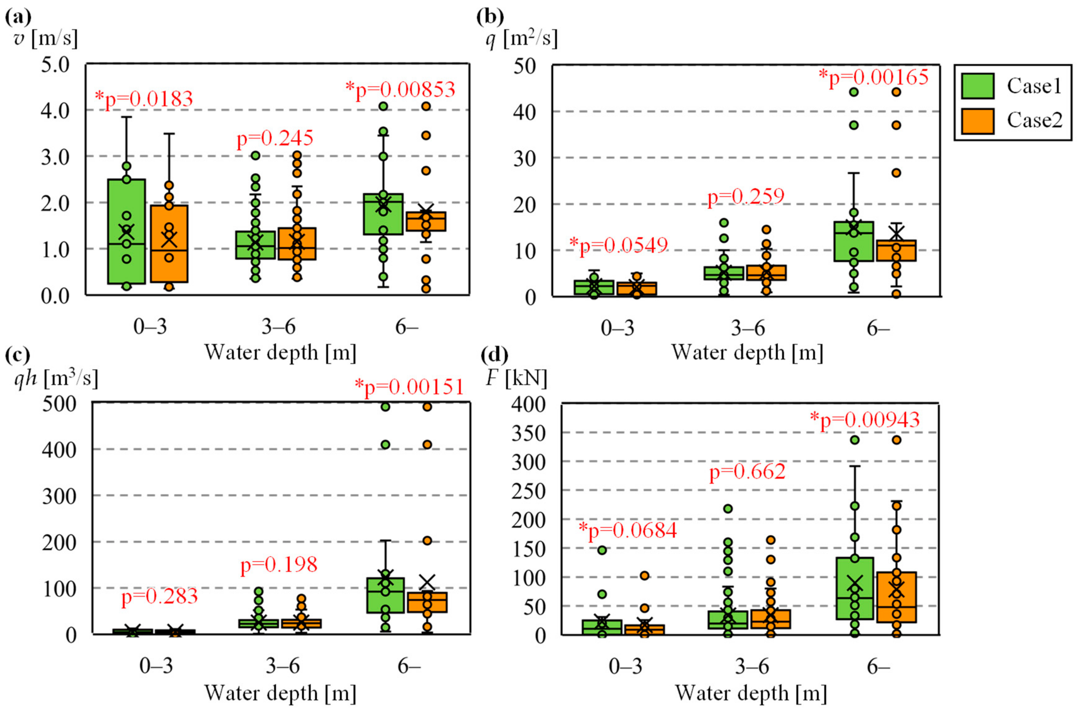
To examine the differences between Cases 1 and 2 in terms of the building loss indices in detail, the results of the comparison based on the inundation depth are presented in Figure 12. Box plots for each building loss index were obtained by dividing the inundation depth into three ranks based on the number of floors in the building: first floor (0–3 m), second floor (3–6 m), and second floor overflow (>6 m). The p-values from the t-tests are also indicated in the figure as a result of examining the significant differences between Cases 1 and 2 for each inundation depth rank. For the flow velocity (Figure 12a), the mean values for Case 1 (Case 2) were 1.36 m/s (1.19 m/s), 1.13 m/s (1.14 m/s), and 1.96 m/s (1.81 m/s) for inundation depths of 0–3 m, 3–6 m, and >6 m, respectively. The velocities in the 0–3 m and >6 m depth ranges were in the order Case 1 > Case 2, and a statistically significant difference was confirmed between the two cases (p < 0.05). No significant difference in velocity was observed between the two cases in the 3–6 m depth range. Similarly, with respect to the unit-width discharge q, moment qh, and fluid force F (Figure 12b–d), significant differences were seen between the two cases for the 0–3 m and >6 m depths, with some exceptions (p < 0.05 or p < 0.10), and no significant differences were found for the 3–6 m depth. These results may reflect the velocity results.
At depths greater than 6 m, Case 1 exhibits a vertical velocity profile with an inflection point resisted up to the second story, whereas Case 2 shows a reverse flow near the bottom under large roughness coefficient conditions (Figure 10), suggesting that the difference in the vertical velocity structure between the two cases is related to the difference in velocity v. In addition, most buildings located near rivers are washed away at a small inundation depth of 0–3 m. In Case 1, the flow velocity at the time of overtopping is evaluated using the SG model. In Case 2, the roughness coefficient owing to the presence of the building is large (Figure 10b), leading to excessive resistance and a decrease in the flow velocity. However, there should be a difference in velocity between Cases 1 and 2, even at a depth of 3–6 m. In this analysis, all buildings except those in Chaya District were assumed to be two-story buildings; therefore, the vertical distribution of the flow velocity generated by one-story buildings (Figure 10c) could be considered in very few buildings. Therefore, the difference in the depth-averaged velocity owing to the difference in the vertical velocity distribution did not appear among the cases. The results of the evaluation of the flow velocity and fluid force indicated statistically significant differences when compared with the equivalent roughness model used in the conventional BR model, suggesting the usefulness of the SG model. The equivalent roughness model cannot properly evaluate fluid forces, and the significance of the SG model is expected to increase in the future.
Meanwhile, it is important to acknowledge certain limitations that are inherent to our research. While it is important to consider factors such as building height, structure, and construction materials, the availability of comprehensive data pertaining to residential buildings is still lacking. The scarcity of such data poses a challenge for accurately incorporating these elements into our analysis. The collection and organization of data regarding residential structures should be a focal point for future endeavors. Without an improved dataset, a comprehensive assessment of the effects of building attributes on fluid force remains constrained. Furthermore, because field observation data generally do not include flow velocity values or fluid force data for actual buildings, it is necessary to verify the accuracy of the proposed model using model experiments and compare it with numerical results using a fine grid (grid resolution of 1 m or less). This will be taken up in future studies.
4. Conclusions
In this study, a new subgrid model was developed for evaluating the fluid force acting on individual buildings to assess damages during flood inundation without increasing the computational load. The following points were clarified through a comparison with the conventional BR method based on a simulation of the Kuma River during the heavy rainfall in July 2020 as an example.
- In terms of the reproducibility of water levels and depths in river and inundation flow analyses, it was confirmed that the calculation accuracy of the Hy2-3D model was generally good. It was also quantitatively illustrated that there were no statistically significant differences in the water levels and depths among the cases for building resistance.
- In terms of the horizontal distribution of the velocity field, which is significant for building damage assessment, the contrast in the velocity difference between the building grid and the surrounding road grid was larger in the SG model (Case 1) than in the equivalent roughness model (Case 2). This is because, in the equivalent roughness model (Case 2), the roughness coefficient is larger even when a small number of buildings are included in the computational grid, and the roughness coefficient is reflected in the horizontal eddy viscosity coefficient; thus, the building effect is spread over a wider area.
- The SG model could reproduce the change in the vertical velocity distribution with the vertical structure of the building. However, the equivalent roughness model could not reproduce the flow velocity distribution with inflection points around the building. It also exhibited a limitation in reproducing the 3D flow velocity distribution around the building precisely because of the backflow near the bottom owing to the large roughness coefficient. Thus, it is clear that the SG model can accurately reproduce the horizontal and vertical structures of the flow velocity.
- A comparison of building loss indices, such as fluid forces acting on each building, revealed significant differences in flow velocity between Cases 1 and 2, particularly in the ranges of 0–3 m and >6 m inundation depths, where statistically significant differences were confirmed. Along with the results of the velocity analysis, similar statistically significant differences were also observed in the unit-width discharge q, moment qh, and fluid force F. These differences were attributed to the horizontal and vertical distribution of the flow velocity. These results suggest that the reproducibility of the vertical velocity distribution is a key factor and that the SG model incorporated into the 3D model can evaluate the inundation flow conditions in a manner that accurately reflects the fluid forces acting on the building, thus demonstrating the usefulness of the model.
Supplementary Materials
The following supporting information can be downloaded at: https://www.mdpi.com/article/10.3390/w15173166/s1, Figure S1: Measured results from 52 to 63 kp along the Kuma River after heavy rainfall in July 2020, obtained from Ogata et al. [55]. (a) Contour map for inundation depth and (b) and map of building damage are shown. Building damages are classified into “loss”, “no loss with inundation”, and “without inundation” in which the two formers are depicted in part (b); Figure S2: (a) Map of building damage in Chaya district located near 53 kp on the Kuma River and (b) photograph taken along the direction of the arrow after the flood disaster of July 2020 heavy rainfall. A piloti structure was located at an upstream point in this district, and the building downstream of the piloti structure was less damaged by this flooding; Figure S3: Histogram of building width B in the computational area. Building width B was evaluated using the plane area of building Ab and Equation (8). Figure S4: RMSE and RRMSE values for the calculated hydrograph of the water level at six observatory stations. The data shown in Figure 7 are used here.
Author Contributions
R.K.: Conceptualization, methodology, programming, numerical simulation, formal analysis, writing—original draft preparation and editing, visualization; J.K.: methodology, programming, numerical simulation, writing—editing; Y.N.: Supervision, project administration, funding acquisition, conceptualization, methodology, writing, original draft preparation, and editing. All authors have read and agreed to the published version of the manuscript.
Funding
This work was supported by the Taisei Foundation and JSPS KAKENHI (grant number 21H04577).
Data Availability Statement
Data supporting the findings of this study are available from the corresponding author upon request.
Acknowledgments
We express our gratitude to Takahiro Sayama and Masafumi Yamada of Kyoto University for providing the discharge data used in the numerical simulation. We thank Yoshiaki Hisada, Kogakuin University, and Kazuo Tamura, Kanagawa University, for their advice regarding building structures.
Conflicts of Interest
The authors declare no conflict of interest.
References
- Zhou, Z.Q.; Xie, S.P.; Zhang, R. Historic Yangtze flooding of 2020 tied to extreme Indian Ocean conditions. Proc. Natl. Acad. Sci. USA 2021, 118, e2022255118. [Google Scholar] [CrossRef]
- Dietze, M.; Bell, R.; Ozturk, U.; Cook, K.L.; Andermann, C.; Beer, A.R.; Thieken, A.H. More than heavy rain turning into fast-flowing water—A landscape perspective on the 2021 Eifel floods. Nat. Hazards Earth Syst. Sci. 2022, 22, 1845–1856. [Google Scholar] [CrossRef]
- Koks, E.E.; Van Ginkel, K.C.; Van Marle, M.J.; Lemnitzer, A. Brief communication: Critical infrastructure impacts of the 2021 mid-July western. Nat. Hazards Earth Syst. Sci. 2022, 22, 3831–3838. [Google Scholar] [CrossRef]
- MoPD. Government of Pakistan: Pakistan Floods 2022 Post-Disaster Needs Assessment. Available online: https://www.pc.gov.pk/uploads/downloads/PDNA-2022.pdf (accessed on 24 April 2023).
- Mallapaty, S. Pakistan’s floods have displaced 32 million people-how researchers are helping. Nature 2022, 609, 667. [Google Scholar] [CrossRef] [PubMed]
- Cabinet Office. Government of Japan: On Disaster Damage by the Heavy Rainfall in July 2018 (In Japanese). Available online: http://www.bousai.go.jp/updates/h30typhoon7/pdf/310109_1700_h30typhoon7_01.pdf (accessed on 2 May 2023).
- Cabinet Office. Government of Japan: On Disaster Damage by the Typhoon No. 19 (Hagibis) in 2019 (In Japanese). Available online: https://www.bousai.go.jp/updates/r1typhoon19/pdf/r1typhoon19_45.pdf (accessed on 2 May 2023).
- Cabinet Office. Government of Japan: On Disaster Damage by the Heavy Rainfall in July 2020 (In Japanese). Available online: http://www.bousai.go.jp/updates/r2_07ooame/pdf/r20703_ooame_40.pdf (accessed on 2 May 2023).
- Hirabayashi, Y.; Mahendran, R.; Koirala, S.; Konoshima, L.; Yamazaki, D.; Watanabe, S.; Kim, H.; Kanae, S. Global flood risk under climate change. Clim. Chang. 2013, 3, 816–821. [Google Scholar] [CrossRef]
- Best, J. Anthropogenic stresses on the world’s big rivers. Nat. Geosci. 2019, 12, 7–21. [Google Scholar] [CrossRef]
- Tabari, H. Climate change impact on flood and extreme precipitation increases with water availability. Sci. Rep. 2020, 10, 13768. [Google Scholar] [CrossRef]
- Kawase, H.; Yamaguchi, M.; Imada, Y.; Hayashi, S.; Murata, A.; Nakaegawa, T.; Miyasaka, T.; Takayabu, I. Enhancement of extremely heavy precipitation. Sci. Online Lett. Atmos. 2021, 17A, 7–13. [Google Scholar]
- Nihei, Y.; Oota, K.; Kawase, H.; Sayama, T.; Nakakita, E.; Ito, T.; Kashiwada, J. Assessment of climate change impacts on river flooding due to Typhoon Hagibis in 2019 using non-global warming experiments. J. Flood Risk Manag. 2023, 16, e12919. [Google Scholar] [CrossRef]
- Jonkman, S.N.; Kelman, I. An analysis of the causes and circumstances of flood disaster deaths. Disasters 2005, 29, 75–97. [Google Scholar] [CrossRef]
- Merz, B.; Kreibich, H.; Thieken, A.; Schmidtke, R. Estimation uncertainty of direct monetary flood damage to buildings. Nat. Hazards Earth Syst. Sci. 2004, 4, 153–163. [Google Scholar] [CrossRef]
- McGrath, H.; Abo El Ezz, A.; Nastev, M. Probabilistic depth-damage curves for the assessment of flood-induced building losses. Hazards 2019, 97, 1–14. [Google Scholar] [CrossRef]
- Hasegawa, K.; Yoshino, H.; Yanagi, U.; Azuma, K.; Osawa, H.; Kagi, N.; Shinohara, N.; Haesgawa, A. Indoor environmental problems and health status in water-damaged home due to tsunami in Japan. Build. Environ. 2015, 93, 24–34. [Google Scholar] [CrossRef]
- Comerio, M.A. Disaster recovery and community renewal: Housing approaches. Cityscape 2014, 16, 51–68. [Google Scholar]
- Ghobarah, A. Performance-based design in earthquake engineering: State of development. Eng. Struct. 2001, 23, 878–884. [Google Scholar] [CrossRef]
- Ellingwood, B.R. Earthquake risk assessment of building structures. Reliab. Eng. Syst. Saf. 2001, 74, 251–262. [Google Scholar] [CrossRef]
- Main, J.A.; Fritz, W.P. Database-Assisted Design for Wind: Concepts, Software, and Examples for Rigid and Flexible Buildings; Institute of Standards and Technology, Technology Administration, US Department of Commerce: Washington, DC, USA, 2006; pp. 14–39.
- Buchanan, A.H.; Abu, A.K. Structural Design for Fire Safety; John Wiley & Sons: Hoboken, NJ, USA, 2017; pp. 8–33. [Google Scholar]
- Burvy, R.J.; Deyle, R.E.; Godschalk, D.R.; Olshansky, R.B. Creating hazard resilient communities through land-use planning. Nat. Hazards Rev. 2000, 1, 99–106. [Google Scholar]
- Kreibich, H.; Kreibich, P.; Vliet, M.V.; Moel, H.D. A review of damage-reducing measures to manage fluvial flood risks in a changing climate. Mitig. Adapt. Strateg. Glob. Chang. 2015, 20, 967–989. [Google Scholar] [CrossRef]
- Schubert, J.E.; Sanders, B.E. Building treatments for urban flood inundation models and implications for predictive skill and modeling efficiency. Adv. Water Resour. 2012, 41, 49–64. [Google Scholar] [CrossRef]
- Aburaya, T.; Imamura, F. Proposal for Tsunami Inundation Simulation Using Synthetic Equivalent Roughness Model. Jpn. Soc. Civil Eng. 2002, 49, 276–280. (In Japanese) [Google Scholar] [CrossRef]
- Gallegos, H.A.; Schubert, J.E.; Sanders, B.F. Two-dimensional, high-resolution modeling of urban dam-break flooding: A case study of Baldwin Hills, California. Adv. Water Resour. 2009, 32, 1323–1335. [Google Scholar] [CrossRef]
- Wang, H.V.; Loftis, J.D.; Liu, Z.; Forrest, D.; Zhang, J. The storm surge and sub-grid inundation modeling in New York City during Hurricane Sandy. Sci. Eng. 2014, 2, 226–246. [Google Scholar] [CrossRef]
- Wang, Y.; Chen, A.S.; Fu, G.; Djordjević, S.; Zhang, C.; Savić, D.A. An integrated framework for high-resolution urban flood modelling considering multiple information sources and urban features. Environ. Model. Softw. 2018, 107, 85–95. [Google Scholar] [CrossRef]
- Aronica, G.T.; Lanza, L.G. Drainage efficiency in urban areas: A case study. Hydrol. Process. 2005, 19, 1105–1119. [Google Scholar] [CrossRef]
- Tsubaki, R.; Fujita, I. Unstructured grid generation using LiDAR data for urban flood inundation modelling. Hydrol. Process. 2010, 24, 1401–1420. [Google Scholar] [CrossRef]
- Sanders, B.F.; Schubert, J.E.; Gallegos, H.A. Integral formulation of shallow-water equations with anisotropic porosity for urban flood modeling. J. Hydrol. 2008, 362, 19–38. [Google Scholar] [CrossRef]
- Viero, D.P. Modelling urban floods using a finite element staggered scheme with an anisotropic dual porosity model. J. Hydrol. 2019, 568, 247–259. [Google Scholar] [CrossRef]
- Apel, H.; Aronica, G.T.; Kreibich, H.; Thieken, A.H. Flood risk analyses—How detailed do we need to be? Nat. Hazards 2009, 49, 79–98. [Google Scholar] [CrossRef]
- Ernst, J.; Dewals, B.J.; Detrembleur, S.; Archambeau, P.; Erpicum, S.; Pirotton, M. Micro-scale flood risk analysis based on detailed 2D hydraulic. Nat. Hazards 2010, 55, 181–209. [Google Scholar] [CrossRef]
- Merz, B.; Kreibich, H.; Schwarze, R.; Thieken, A. Assessment of economic flood damage. Nat. Hazards Earth Syst. Sci. 2010, 10, 1697–1774. [Google Scholar] [CrossRef]
- Wing, O.E.J.; Bates, P.D.; Sampson, C.C.; Smith, A.M.; Johnson, K.A.; Erickson, K.A. Validation of a 30 m resolution flood hazard model for the conterminous United States. Water Resour. Res. 2017, 53, 7968–7986. [Google Scholar] [CrossRef]
- Wilson, M.; Bates, P.; Alsdorf, D.; Forsberg, B.; Horritt, M.; Mekack, J.; Frappart, F.; Famiglietti, J. Modeling large-scale inundation of Amazonian seasonally flooded wetlands. Geophys. Res. Lett. 2007, 34, L15404. [Google Scholar] [CrossRef]
- Alho, P.; Aaltonen, J. Comparing a 1D hydraulic model with a 2D hydraulic model for the simulation of extreme glacial outburst floods. Hydrol. Process. 2008, 22, 1407–1572. [Google Scholar] [CrossRef]
- Sanders, B.F.; Schubert, J.E.; Detwiler, R.L. ParBreZo: A parallel, unstructured grid, Godunov-type, shallow-water code for high-resolution flood inundation modeling at the regional scale. Adv. Water Resour. 2010, 33, 1456–1467. [Google Scholar] [CrossRef]
- McMillan, H.K.; Brasington, J. Reduced complexity strategies for modelling urban floodplain inundation. Geomorphology 2007, 90, 226–243. [Google Scholar] [CrossRef]
- Zhang, S.; Wang, T.; Zhao, B. ParBreZo: Calculation and visualization of flood inundation based on a topographic triangle network. J. Hydrol. 2014, 509, 406–415. [Google Scholar] [CrossRef]
- Xian, S.; Lin, N.; Kunreuther, H. Optimal house elevation for reducing flood-related losses. J. Hydrol. 2017, 548, 63–74. [Google Scholar] [CrossRef]
- Liao, K.H.; Le, T.A.; Nguyen, K.V. Urban design principles for flood resilience: Learning from the ecological wisdom of living with floods in the Vietnamese Mekong Delta. Landsc. Urban Plan. 2016, 155, 69–78. [Google Scholar] [CrossRef]
- Yamamoto, T.; Kazama, S.; Touge, Y.; Yanagihara, H.; Tada, T.; Takizawa, H. Evaluation of flood damage reduction throughout Japan from adaptation measures taken under a range of emissions mitigation scenarios. Clim. Chang. 2021, 165, 60. [Google Scholar] [CrossRef]
- Bartier, P.M.; Keller, C.P. Multivariate interpolation to incorporate thematic surface data using inverse distance weighting (IDW). Comput. Geosci. 1996, 22, 795–799. [Google Scholar] [CrossRef]
- Nihei, Y.; Kato, Y.; Sato, K. A new three-dimensional numerical method for large-scale river flow and its application to a flood flow computation. J. Jpn. Soc. Civil Eng. 2005, 803, 115–131. [Google Scholar]
- Kashiwada, J.; Nihei, Y. A High Accurate and Efficient 3D River Flow Model with a New Mode-Splitting Technique. In Proceedings of the 39th IAHR World Congress, Granada, Spain, 19–24 June 2022. [Google Scholar]
- Kashiwada, J.; Kubota, R.; Hiramoto, T.; Yamada, M.; Sayama, T.; Nihei, Y. Building washout rates in the Kuma River flood in 2020 based on the integrated analysis of river flow and inundation flow. Adv. River Eng. 2023, 29, 401–406. [Google Scholar]
- Imai, K.; Imamura, F.; Iwama, S. Advanced tsunami computation for urban regions. J. Jpn. Soc. Civil Eng. Ser. B2 2013, 69, I-311–I-315. [Google Scholar]
- Kuwamura, H. Drag and uplift of a cuboid structure standing in inundation flow—Hydraulic study in natural river flow Part2. J. Struct. Construct. Eng. (Trans. AIJ) 2016, 81, 219–227. [Google Scholar] [CrossRef]
- Wu, W. Computational River Dynamics; Taylar & Francis: Abingdon, UK, 2008; pp. 11–58. [Google Scholar]
- Yokoki, H.; Uchida, T.; Inagaki, A.; Tsukai, M.; Seto, S.; Yokojima, S.; Yoshikawa, Y.; Tsubaki, R.; Saiki, I. Editorial in Special issue on the July 2020 heavy rainfall event in Japan. J. Jpn. Soc. Civil Eng. 2021, 10, 545–549. [Google Scholar] [CrossRef] [PubMed]
- Hirokawa, Y.; Kato, T.; Araki, K.; Mashiko, W. Characteristics of an extreme rainfall event in Kyushu District, Southwestern Japan, in Early July 2020. Sci. Online Lett. Atmos. 2020, 16, 265–270. [Google Scholar] [CrossRef]
- Ogata, Y.; Hotta, T.; Ito, T.; Inoue, T.; Ota, K.; Onomura, S.; Nihei, Y. Relation between inundation, building and human damage, in Kuma River due to Reiwa. J. Jpn. Soc. Civil Eng. Ser. B1 2021, 77, I-457–I-462. [Google Scholar]
- Sayama, T.; Ozawa, T.; Kawakami, T.; Nabesaka, S.; Fukami, K. Rainfall-runoff-inundation analysis of the 2010 Pakistan. Hydrol. Sci. J. 2012, 57, 298–312. [Google Scholar] [CrossRef]
- Kanda, M. Progress in the scale modeling of urban climate. Theor. Appl. Climatol. 2006, 84, 23–33. [Google Scholar] [CrossRef]
- Raupach, M.R. Simplified expressions for vegetation roughness length and zero-plane displacement as a function of canopy height and area index. Bound.-Layer Meteorol. 1994, 71, 211–216. [Google Scholar] [CrossRef]
Figure 1.
Schematic of fundamental concept of subgrid model for building fluid force. (a) When medium grid resolutions are adopted, buildings of various heights are located in several computational grids. (b) In Step 1, each building is divided horizontally and vertically for each computational grid. (c) In Step 2, the flow velocity at each grid is interpolated at the center of each building. (d) In Step 3, the fluid force obtained for each building is distributed to each grid.
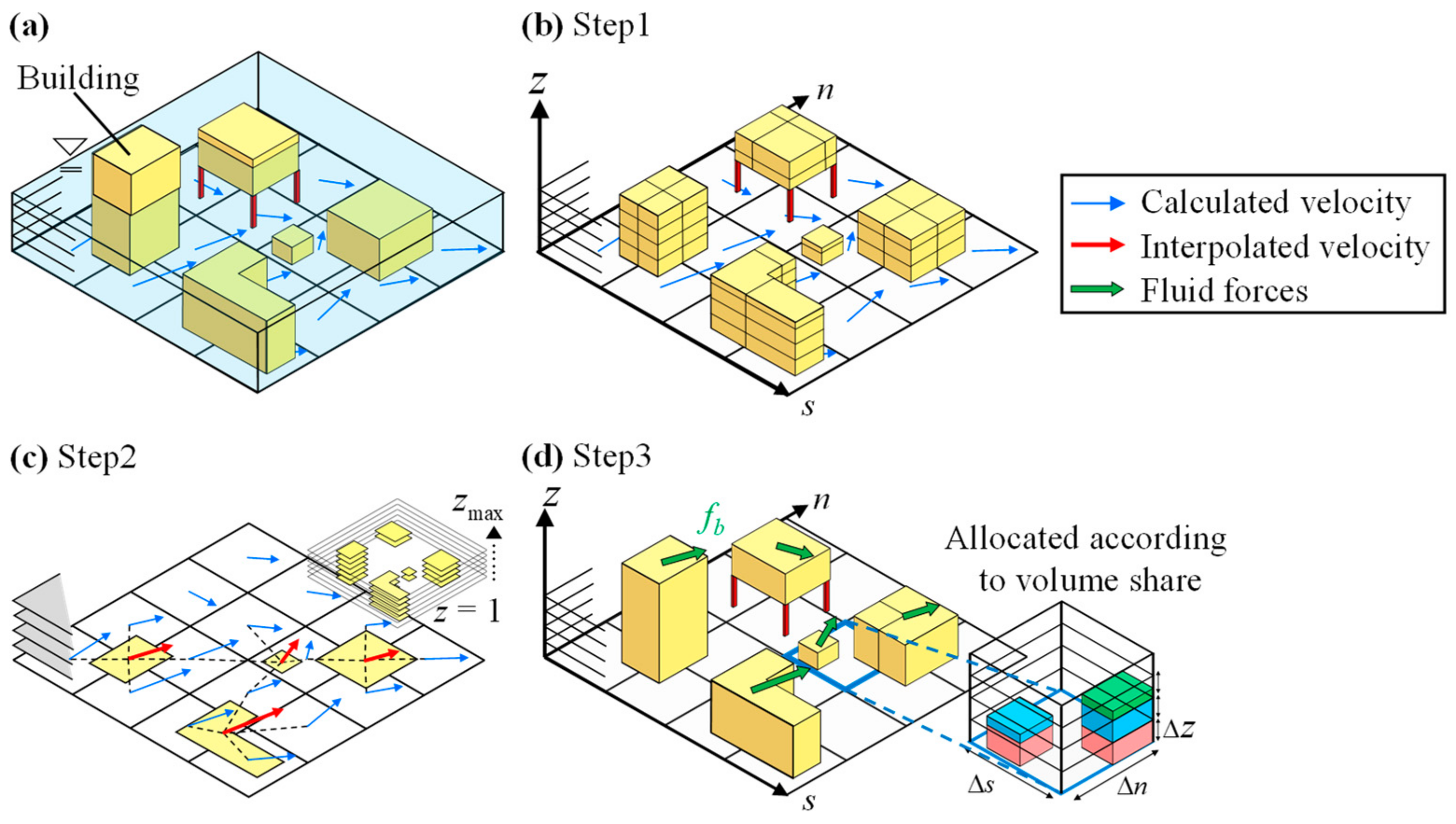
Figure 2.
Interpolation method of calculated velocities at the center of each building using IDW for evaluation of building fluid force. Velocities in s and n directions, us and un, respectively, are defined in staggered grids.
Figure 2.
Interpolation method of calculated velocities at the center of each building using IDW for evaluation of building fluid force. Velocities in s and n directions, us and un, respectively, are defined in staggered grids.
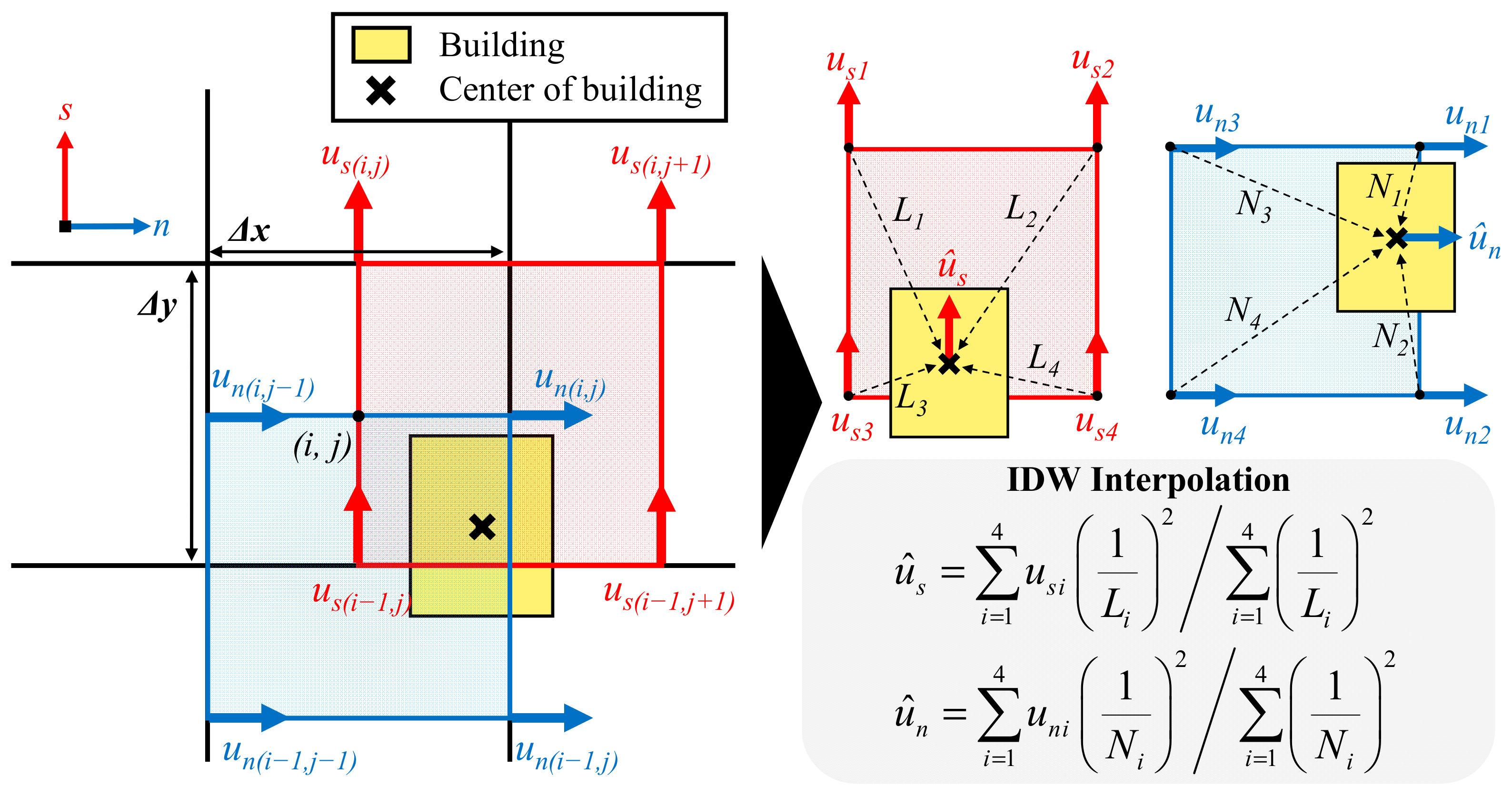
Figure 3.
Time interval concept in 2D and 3D calculations in Hy2-3D model. (a) Case when Δt2D = Δt3D1 and (b) case when Δt2D > Δt3D1.
Figure 3.
Time interval concept in 2D and 3D calculations in Hy2-3D model. (a) Case when Δt2D = Δt3D1 and (b) case when Δt2D > Δt3D1.

Figure 4.
(a) Location and elevation map of the Kuma River Basin; (b) computational domain from 51.8 kp to 68.6 kp along the Kuma River.
Figure 4.
(a) Location and elevation map of the Kuma River Basin; (b) computational domain from 51.8 kp to 68.6 kp along the Kuma River.
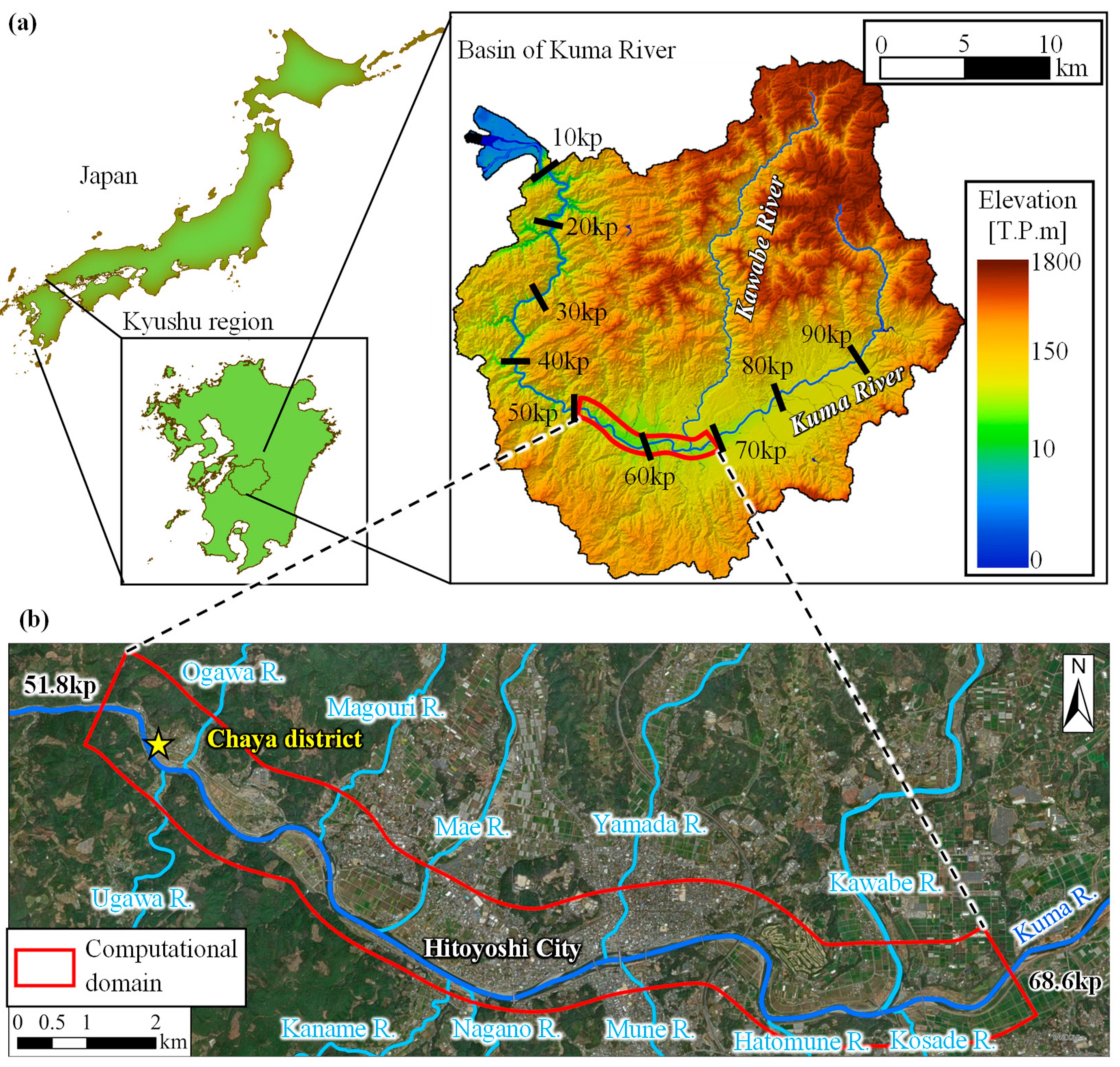
Figure 5.
(a) Temporal variations in basin-averaged precipitation and water level at Ohashi (61.5 kp) in the Kuma River. Precipitation and water level data were obtained from http://www.jmbsc.or.jp/en/index-e.html (accessed on 22 November 2022) and https://www.river.go.jp/index (accessed on 22 November 2022), respectively; (b) boundary conditions of inflow discharge at upstream points and tributaries, and water level at the downstream point. River discharges in the Kuma River and 11 major tributaries were obtained from the runoff calculation results [49]. Water level at the downstream end was obtained from the computational results using 1D unsteady flow analysis performed by the authors.
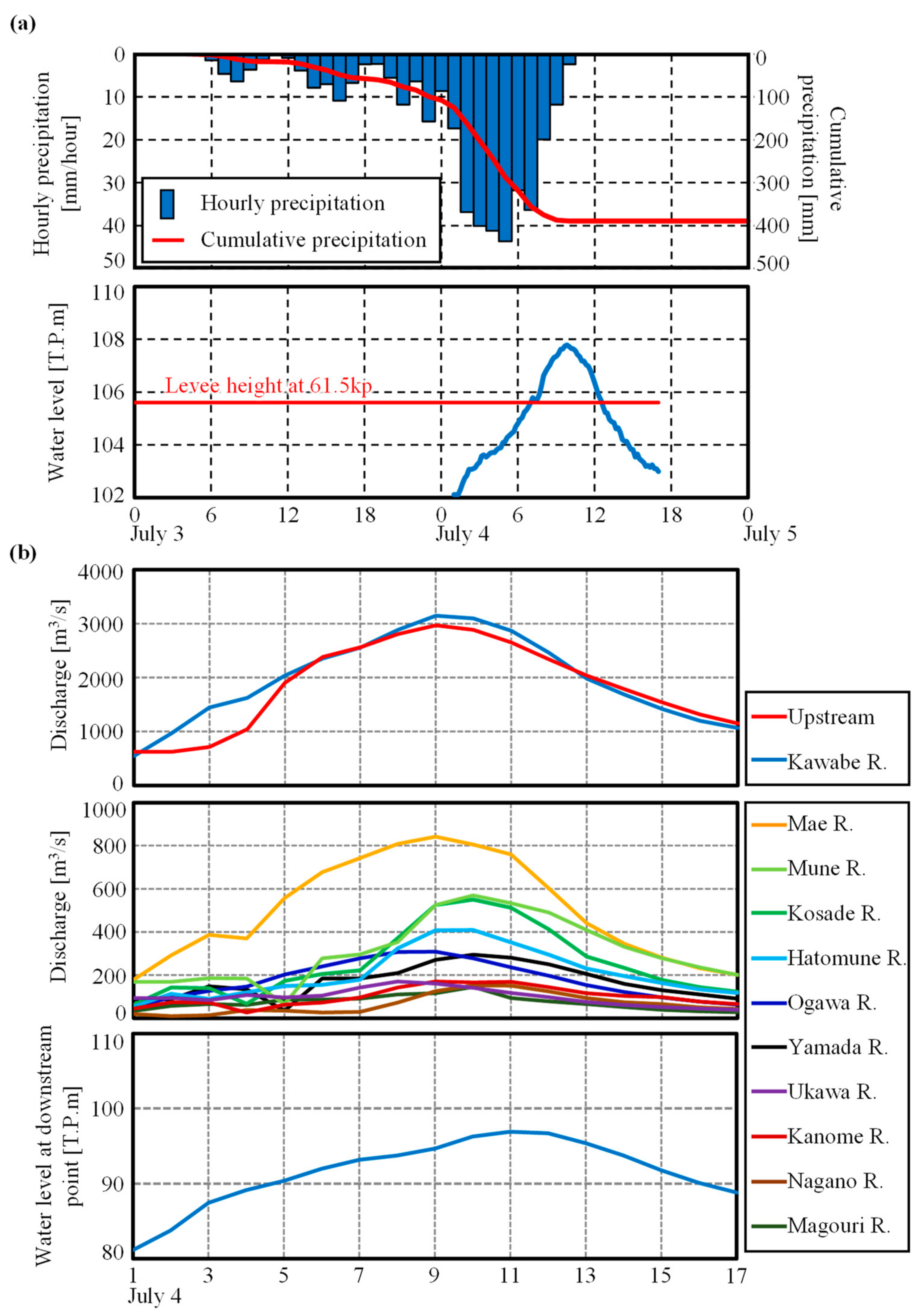
Figure 6.
(a) Longitudinal distribution of calculated and observed water levels at various time points in the Kuma River; (b) calculated and observed peak water levels; and (c) difference in peak water levels between Case 1 and other cases. The calculated results for Case 1 are used in parts (a,b).
Figure 6.
(a) Longitudinal distribution of calculated and observed water levels at various time points in the Kuma River; (b) calculated and observed peak water levels; and (c) difference in peak water levels between Case 1 and other cases. The calculated results for Case 1 are used in parts (a,b).
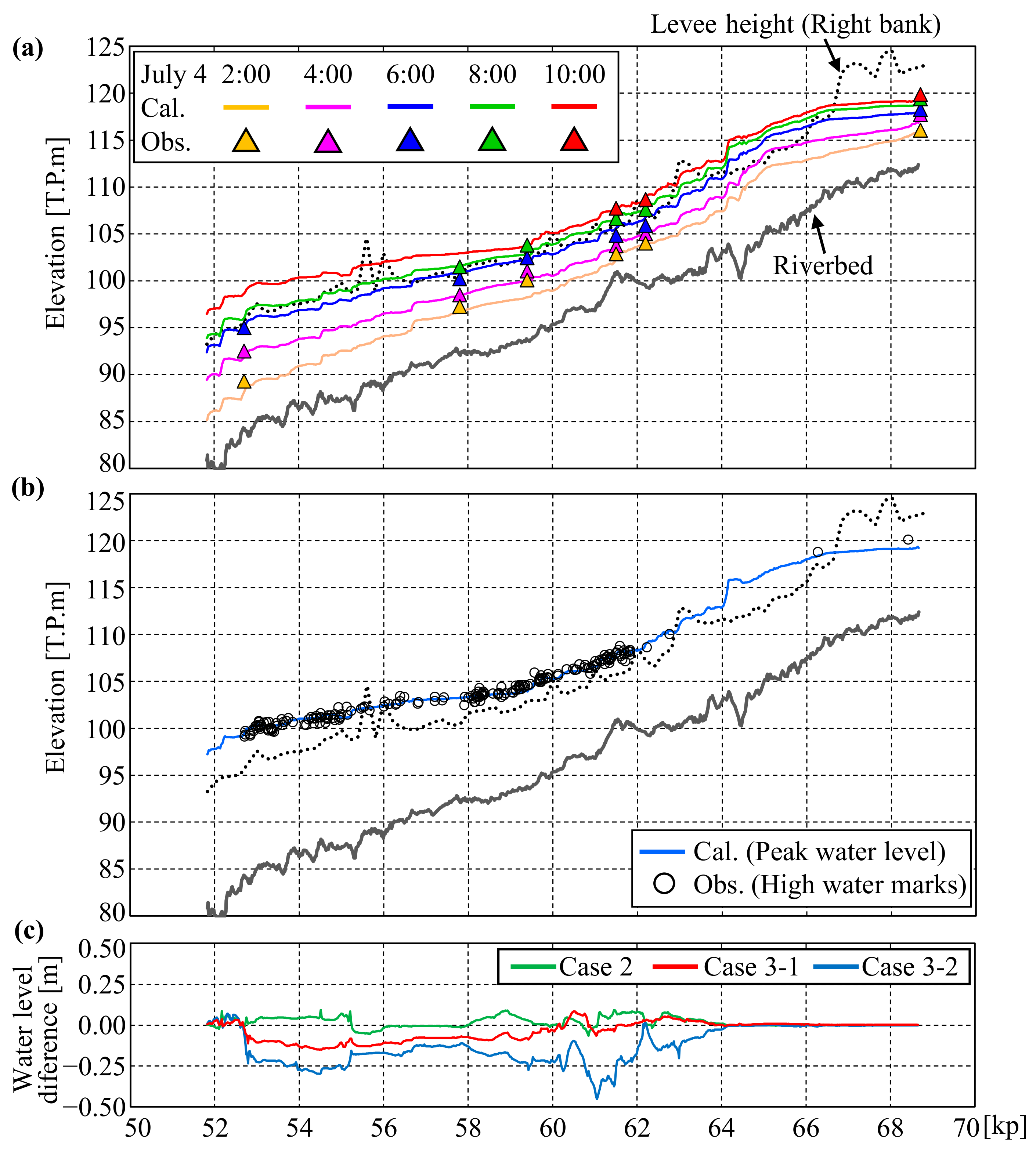
Figure 7.
Temporal variation in calculated and observed water levels in the Kuma River. The calculated results for Case 1 are shown. The results at water-level observatories Ichibu (68.6 kp), Hitoyoshi (62.2 kp), Ohashi (61.5 kp), Nishizebashi (59.4 kp), Gogan (57.4 kp), and Watari (52.7 kp) are depicted.
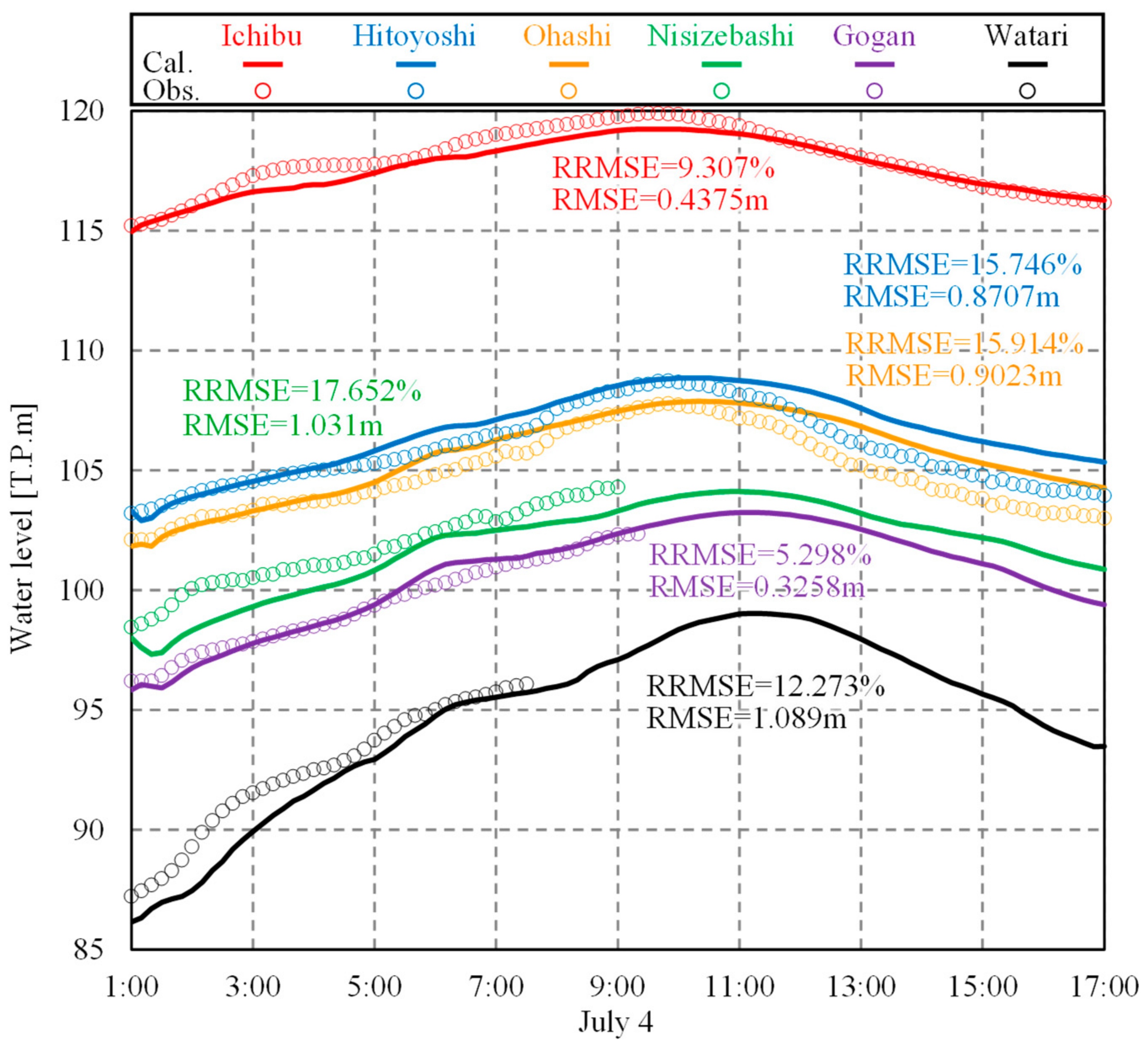
Figure 8.
Scatter plots of (a) calculated and observed peak water levels and (b) water depth in inundated area. The calculated results for Case 1 are used in the figure. Observed results are based on those reported by Ogata et al. [55].
Figure 8.
Scatter plots of (a) calculated and observed peak water levels and (b) water depth in inundated area. The calculated results for Case 1 are used in the figure. Observed results are based on those reported by Ogata et al. [55].
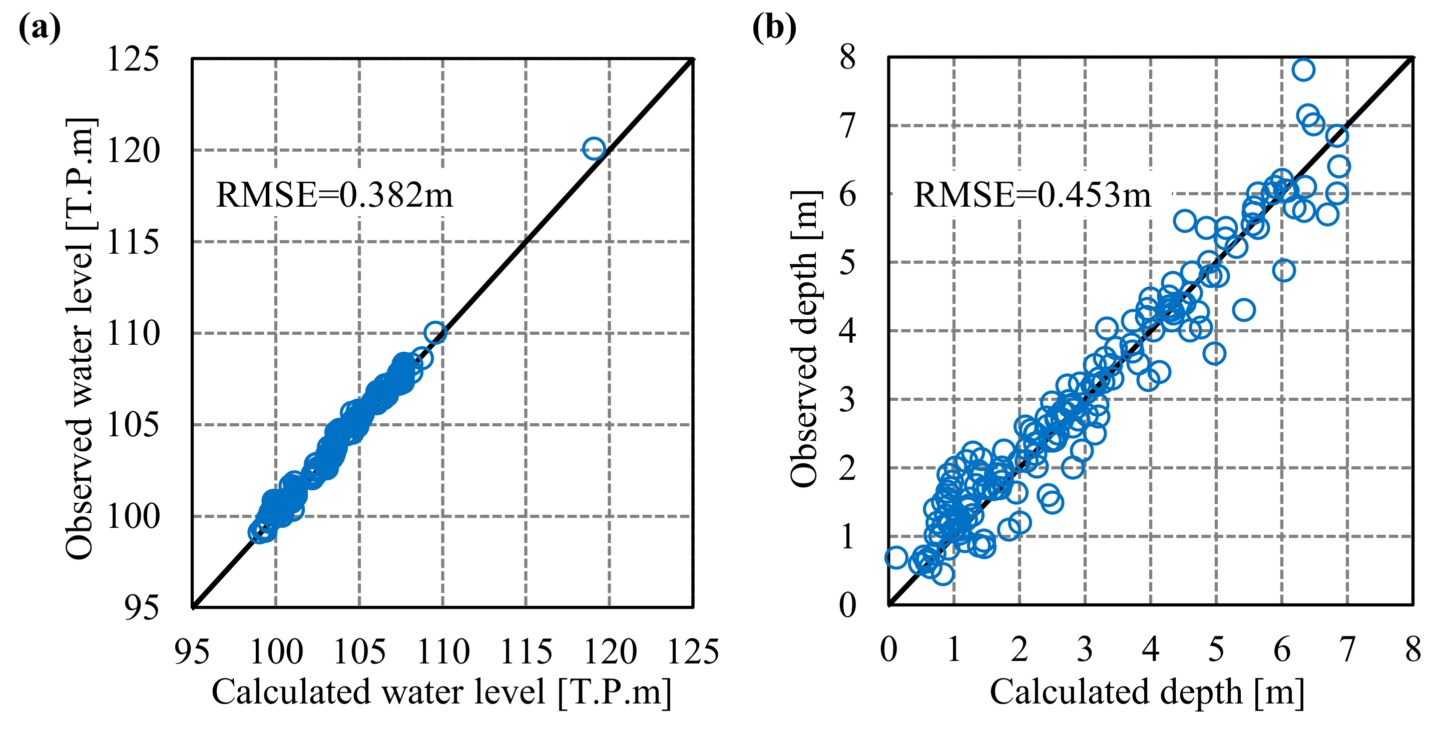
Figure 9.
(a) Contour maps of calculated depth horizontal velocities at 10:00 a.m. on 4 July 2020, near the Hitoyoshi city area and (b) cross-sectional distributions of calculated horizontal velocities and water levels with locations of buildings along section A-A′. Magnitude of depth-averaged horizontal velocities in all cases is depicted.

Figure 10.
Vertical distribution of streamwise velocity at 11:30 a.m. on 4 July 2020 in Chaya District. (a) Locations of four stations. (b) Equivalent roughness n in this area. Calculated velocities for (c) Case 1 and (d) Case 2 are shown.
Figure 10.
Vertical distribution of streamwise velocity at 11:30 a.m. on 4 July 2020 in Chaya District. (a) Locations of four stations. (b) Equivalent roughness n in this area. Calculated velocities for (c) Case 1 and (d) Case 2 are shown.
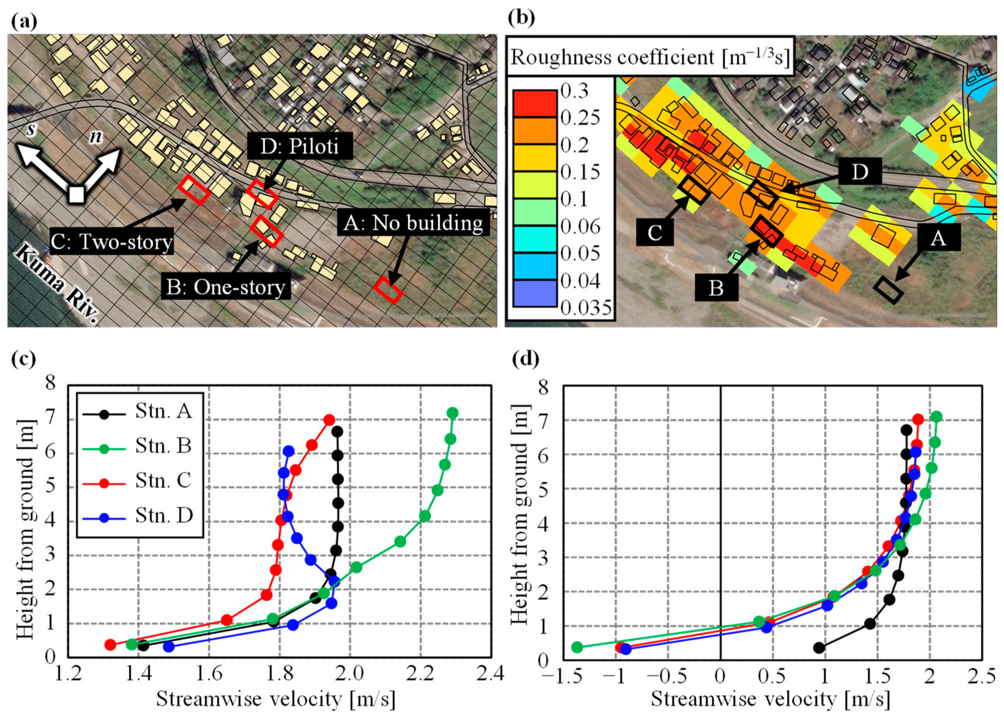
Figure 11.
Correlation diagram of building loss indices for Cases 1 and 2 in lost buildings (160 buildings). p-value showing a statistically significant difference between Cases 1 and 2 is also illustrated (* p < 0.10).
Figure 11.
Correlation diagram of building loss indices for Cases 1 and 2 in lost buildings (160 buildings). p-value showing a statistically significant difference between Cases 1 and 2 is also illustrated (* p < 0.10).
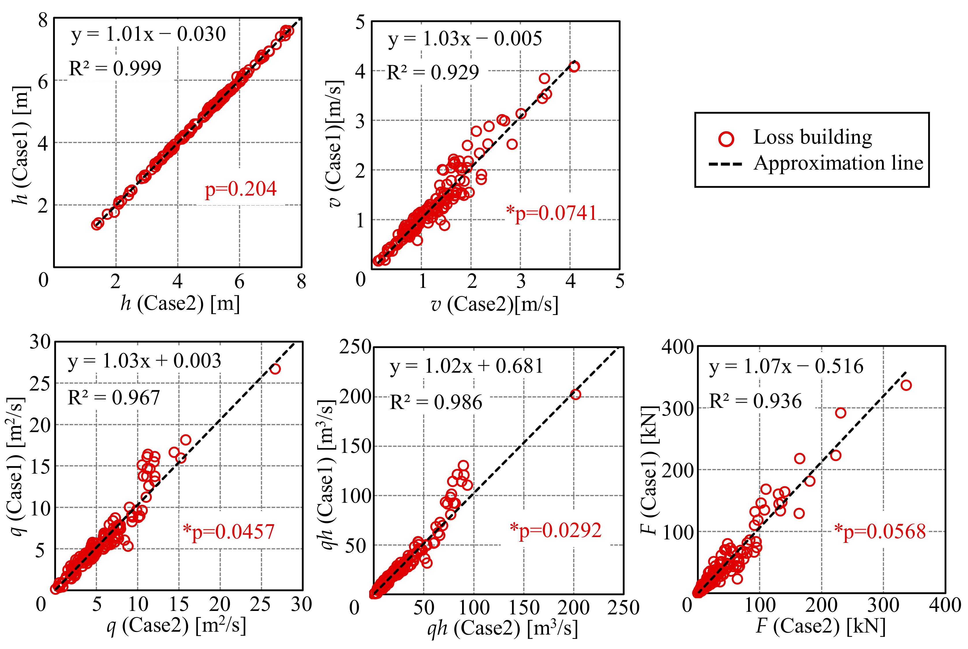
Figure 12.
Boxplot showing flood index by flood depth level in lost buildings for Cases 1 and 2. p-value indicating a statistically significant difference between Cases 1 and 2 is also shown (* p < 0.05).
Figure 12.
Boxplot showing flood index by flood depth level in lost buildings for Cases 1 and 2. p-value indicating a statistically significant difference between Cases 1 and 2 is also shown (* p < 0.05).

Table 1.
RMSE values, slopes, and R2 in regression lines for calculated and observed peak water levels and depths for various cases.
Table 1.
RMSE values, slopes, and R2 in regression lines for calculated and observed peak water levels and depths for various cases.
| Peak Water Level | Peak Water Depth | |||||
|---|---|---|---|---|---|---|
| RMSE [m] | Slope | R2 | RMSE [m] | Slope | R2 | |
| Case 1 | 0.3815 | 1.0210 | 0.9898 | 0.4525 | 0.9300 | 0.9367 |
| Case 2 | 0.3626 | 1.0200 | 0.9902 | 0.4421 | 0.9306 | 0.9390 |
| Case 3-1 | 0.4178 | 1.0180 | 0.9875 | 0.4658 | 0.9339 | 0.9261 |
| Case 3-2 | 0.5447 | 1.0060 | 0.9897 | 0.5480 | 0.9452 | 0.9343 |
Disclaimer/Publisher’s Note: The statements, opinions and data contained in all publications are solely those of the individual author(s) and contributor(s) and not of MDPI and/or the editor(s). MDPI and/or the editor(s) disclaim responsibility for any injury to people or property resulting from any ideas, methods, instructions or products referred to in the content. |
© 2023 by the authors. Licensee MDPI, Basel, Switzerland. This article is an open access article distributed under the terms and conditions of the Creative Commons Attribution (CC BY) license (https://creativecommons.org/licenses/by/4.0/).
Share and Cite
MDPI and ACS Style
Kubota, R.; Kashiwada, J.; Nihei, Y. Subgrid Model of Fluid Force Acting on Buildings for Three-Dimensional Flood Inundation Simulations. Water 2023, 15, 3166. https://doi.org/10.3390/w15173166
AMA Style
Kubota R, Kashiwada J, Nihei Y. Subgrid Model of Fluid Force Acting on Buildings for Three-Dimensional Flood Inundation Simulations. Water. 2023; 15(17):3166. https://doi.org/10.3390/w15173166
Chicago/Turabian StyleKubota, Riku, Jin Kashiwada, and Yasuo Nihei. 2023. "Subgrid Model of Fluid Force Acting on Buildings for Three-Dimensional Flood Inundation Simulations" Water 15, no. 17: 3166. https://doi.org/10.3390/w15173166
Note that from the first issue of 2016, this journal uses article numbers instead of page numbers. See further details here.