
Sea Level Rise Effects on the Sedimentary Dynamics of the Douro Estuary Sandspit (Portugal)

1
Faculdade de Engenharia, Universidade do Porto, Rua Dr. Roberto Frias s/n, 4200-465 Porto, Portugal
2
Centro Interdisciplinar de Investigação Marinha e Ambiental, Universidade do Porto, Terminal de Cruzeiros de Leixões, Av. General Norton de Matos s/n, 4450-208 Matosinhos, Portugal
*
Author to whom correspondence should be addressed.
Water 2023, 15(15), 2841; https://doi.org/10.3390/w15152841
Submission received: 28 June 2023
/
Revised: 27 July 2023
/
Accepted: 29 July 2023
/
Published: 6 August 2023
(This article belongs to the Special Issue Investigation, Simulation and Application in Hydrodynamics for Coastal and Ocean Engineering)
Abstract
:Sandspits are important natural defences against the effects of storm events in estuarine regions, and their temporal and spatial dynamics are related to river flow, wave energy, and wind action. Understanding the impact of extreme wave events on the morphodynamics of these structures for current conditions and future projections is of paramount importance to promote coastal and navigation safety. In this work, a numerical analysis of the impact of a storm on the sandspit of the Douro estuary (NW Portugal) was carried out considering several mean sea level conditions induced by climate change. The selected numerical models were SWAN, for hydrodynamics, and XBeach, for hydrodynamic and morphodynamic assessments. The extreme event selected for this study was based on the meteo-oceanic conditions recorded during Hurricane Christina (January 2014), which caused significant damage on the western Portuguese coast. The analysis focused on the short-term (two days) impact of the storm on the morphodynamics of the sandspit in terms of its erosion and accretion patterns. The obtained results demonstrate that the mean sea level rise will induce some increase in the erosion/accretion volumes on the seaward side of the sandspit. Overtopping of the detached breakwater and the possibility of wave overtopping of the sandspit crest were observed for the highest simulated mean sea levels.
Keywords:
sandspit; hydro-morphodynamics; extreme event; sea level rise; SWAN; XBeach; Douro estuary1. Introduction
Sandspits are long, narrow landforms that usually form in shallow water on sandy coasts with littoral drift. These structures are highly dynamic in position and shape, being shaped over short- and long-term periods by the action of currents, waves, wind, tides, river flow, sediment transport, and anthropogenic activities [1,2,3]. Short-term events in particular, such as river floods and extreme storms, can have a strong impact on their structure [4,5,6].
Sandspits play an important role in the protection of estuarine and coastal environments. They consequently receive particular attention when located in areas of higher population density, as there is an interest in stabilising their natural dynamics to avoid changes that may increase the risk of flooding and erosion in the coastal strip. These concerns often lead to the need for human intervention. The sandspit at the mouth of the river Douro is such a case.
The Douro flows into the Atlantic Ocean and its simple funnel-shaped estuary lies in a densely populated area between the city of Porto on the right (northern) bank and the city of Vila Nova de Gaia on the left (southern) bank. On the left bank, there is a sandspit that protects the estuary from ocean flooding, storm wave damage, and erosion. However, like most spits, this landform was not stable, showing a highly dynamic behaviour forced by the sea and river currents and influenced by meteorological phenomena [1]. Since the 18th century, several structures have been built to stabilise the sandspit (cf. Figure 1), prevent the sandspit from migrating into the estuary and the navigation channel, facilitate navigation in the estuary, reduce the dredging required to maintain the channel and protect the São Paio Bay Natural Reserve [1,7]. These structures are the Touro and Felgueiras jetties, built in 1790 and 1886, respectively; the southern groin, built in the 1820s; and a new breakwater (built on top of the Touro jetty) north of the estuarine mouth, a detached breakwater in front of the sandspit, and the extension and reinforcement of the southern groin, made between 2005 and 2008 [8]. The northern breakwater protects the access channel and the estuary from wave action, mostly coming from the northwest quadrant [9]. The structures on the south bank reinforce the sandspit and prevent channel siltation by stopping the transport of sediment from the sandspit into the channel. The monitoring carried out so far shows that the intended effects are being achieved [10]. However, an increase in the area and volume of the sandspit has been observed in recent years [1], which may affect the water level inside the estuary during flood events [11] but also during extreme wave conditions, such as those recorded during Storm Christina.
Storm Christina formed as a hurricane in the NW Atlantic near the US East Coast on 1 January 2014. Five days later, on 6 January, the centre of the storm was west of Ireland. The frontal system reached northern and central Portugal on the same day and reached southern Portugal on 7 January [12]. The storm generated very long-period waves (meteotsunamis), with a major impact on the western coast of Portugal [13]. During this two-day period (6–7 January), the Leixões wave buoy recorded WNW waves with a significant height ) of 8.3 m and a peak period of 18.2 s. The maximum wave height () reached 13.5 m with an associated period () of 22.7 s. However, around 08h00 UTC on 6 January, the maximum wave periods () were longer than 20 s, reaching 27.3 s at about 12h00 UTC (Figure 2) [14]. Because of the N–S orientation of the western Portuguese coast, the reduction in spatial energy density due to wave refraction is minimised for WNW incoming waves. Under these conditions, the waves generated by Storm Christina had a high potential to cause morphological changes and destruction in coastal areas. Following the passage of the storm, almost all beaches along the Portuguese mainland coastline experienced significant sediment loss. In beach-dune systems, there were significant retreats in the frontal dune cord with the formation of pronounced scarps due to erosion. Erosion, overtopping, and flooding phenomena were particularly pronounced on the low and sandy coast in beach-dune systems with a sediment deficit and with a previously established erosive trend. Erosive phenomena also occurred on the cliff coasts bordered by narrow beaches or artificial structures, and, in the associated low areas, there were episodes of oceanic overtopping, sometimes accompanied by flooding. Along the coast, beach bars and waterfront restaurants were damaged. Dozens of boats were sunk or damaged in marinas and harbours. Beach access paths and dune protection systems were either damaged or destroyed. There was no loss of life, but dozens of people were injured or had to be rescued from the sea. In the Porto area and around the mouth of the Douro estuary, a beach bar was destroyed, four people were injured and many more were swept away by a wave, and 20 cars (including a tourist bus) were swept inland [13,15].
There is empirical evidence that the mean annual temperature and mean sea level are rising [16]. Studies by Gulev et al. [17] and Geng and Sugi [18] have found an increase in the number of extreme cyclones. Due to global warming, atmospheric circulation patterns are changing, leading to changes in wind patterns and, hence, in wave direction, and in the intensity and frequency of extreme wave events [19,20]. Given the projected mean sea level rise, the impact of storms like Christina on coastal regions may become even more damaging, so further research is needed to increase confidence in forecasts and to provide accurate information to policy makers to support objective adaptation measures to protect the population and their socio-economic activities. Numerical modelling is an important tool that can overcome the lack of data and predict the evolution of sandspits under current conditions as well as for future projections. Several works assessing sandspit evolution using numerical modelling exist. Duc Anh et al. [21] studied the long-term evolution of two sandspits in Vietnam using remote sensing and the numerical model Delft3D. Lisboa and Fernandes [22] analysed the effect of the construction of a port on the sandspit at the Patos lagoon (Brazil) using remote sensing and the numerical model openTELEMAC-MASCARET. Bugajny et al. [23] focused on the analysis of the beach and dune evolution of the Dziwnow Spit (Baltic Sea, Poland) using XBeach. Allard et al. [24] studied the evolution of the Arçay Spit (France) with different wave climates on seasonal to interannual time scales using SWAN and several empirical longshore transport formulas. Finally, Gruwez et al. [25] performed hindcasts with the XBeach model for a sandspit and coastal region in Ada, Ghana. However, there are few works that have considered the impact of extreme events on sandspits using numerical models. Previous works that have addressed this issue are the study by Bugajny et al. [23] and the work by Boudet et al. [26], which presents the evolution of the Rhone River delta (France) using Delft3D and considers different wave and river flow events, including storms and floods.
The objective of this work is to assess the short-term effects of a Christina-like storm on the sandspit of the Douro estuary for current and future conditions, considering the mean sea level rise projected by the IPCC scenarios [27]. For this purpose, the SWAN and XBeach models were applied to the region, calibrated, validated, and run for several scenarios.
2. Materials and Methods
2.1. Numerical Models
The computational framework consists of three nested models in grids of increasing resolution for dynamic downscaling: model M1, an Ibero-Atlantic regional model; model M2, a coastal model for the Espinho-Lavra coastal stretch; and model M3, a local model for the Foz do Douro (mouth of the river Douro).
Model M1 is a hydrodynamic model based on the 3rd generation spectral wave model SWAN [28,29]. It covers the entire western coast of the Iberian Peninsula, the coast of the Algarve (Portugal), and the northern coast of Galicia (Spain). The geographical grid has a resolution of 0.05° × 0.05° (Figure 3a). This model simulates the large-scale propagation of sea waves from deep water to the coast. Bathymetric information was obtained from GEBCO 2021 [30] at a resolution of 15″ × 15″. Depths are referred to as mean sea level (MSL) in the year 2021. Bathymetric data were interpolated in space to match the computational grid and smoothed to avoid gradients that could cause model instability. Neither astronomical tides nor storm surges were considered in this model.
M2 is a coastal implementation of the SWAN model. It simulates the propagation of sea waves in the coastal area at the higher spatial resolution of 30″ × 30″. Its grid covers the coastal area adjacent to the Douro estuary, between the towns of Espinho in the south and Lavra in the north, over a length of about 28 km in the south-north direction and extends to about 15 km off the coast (Figure 3b). Its resolution is close to 930 m in latitude and 700 m in longitude. The bathymetric data for the grid were obtained from GEBCO 2021 [30], interpolated to match the computational grid, and smoothed. Temporal variations in sea level due to tides and storm surges were included but assumed to be uniformly distributed in space. As the M2 model is nested within the domain of the M1 model, the boundary conditions of the M2 model are those provided by the M1 model runs.
Finally, M3 is a local hydro-morphodynamic model of the mouth of the Douro estuary. It is based on the XBeach model [31,32], and it simulates the wave–current–sediment interaction in the coastal zone. Its spatial grid has a variable resolution: maximum resolution in the region of the sandspit (6 m × 6 m) and minimum resolution (22 m × 22 m) near the boundaries. The western, offshore boundary is oriented parallel to the contours of the local bathymetry and is located about 3 km from the coast. The eastern fluvial boundary is located about 3 km upstream of the sandspit (Figure 3c). Bathymetric information was obtained from several sources: EMODnet 2020 DTM [33] at a resolution of 3.75″ × 3.75″, resampled and filtered for the oceanic area; a 2019 bathymetric survey (supplied by the Instituto Hidrográfico of the Portuguese Navy) for the estuarine area; a DTM of the 2011 national survey with LIDAR for the coastal topobathymetry (excluding the sandspit) provided by Direcção-Geral do Território (DGT); a CIIMAR/FCUP high-resolution topographic survey of July 2011 for the sandspit elevation model; a 2014 coastal DTM provided by DGT, for the topography of the estuary margins; and topographic surveys of the municipalities of Porto (date unknown) and Vila Nova de Gaia (dated 2012) for the estuary margins in the most upstream zone not covered by the coastal DTM of DGT. Data were aggregated prioritizing higher-resolution data in overlapping areas. For bathymetry, the estuarine survey was completed with LIDAR data and afterward with EMODNET ocean data. The time evolution of the sea level at both the offshore and inshore boundaries was assumed to be the same as in model M2. Difficulties in setting up the XBeach model forced us to consider a zero river discharge. On the western boundary, the two-dimensional SWAN energy spectra obtained from model M2 were imposed at the north and south corners and at a third point in the middle of the offshore boundary with a time discretisation of 30 min.
The numerical experiments were forced with wind velocity fields at 10 m above sea level from the ECMWF ERA5 climate reanalysis project [34], with a spatial resolution of 0.25° × 0.25° and a time resolution of 1 h. Recent research has shown that ERA5 reanalysis winds are accurate for both wave modelling at the oceanic scale [35,36,37,38] and in enclosed seas [39,40]. The same data have also been used to validate historical wind climate data in the analysis of climate change projections [41].
The offshore boundary conditions consist of two different sets of hindcast wave parameters, one from the ECMWF ERA5 climate reanalysis project, and the other from the IBI (Iberian-Biscay-Irish) ocean wave reanalysis [42]. The ERA5 sea wave surface data include significant wave height, , mean period, , mean wave direction, , and the standard deviation of the directional dispersion from the peak direction, , at a spatial resolution of 0.5° × 0.5° and a time resolution of 1 h. The IBI data include significant wave height, , peak period, , and the direction associated with the peak period, , at a spatial resolution of 0.05° × 0.05° and a time resolution of 1 h.
In the nested models M2 and M3, the time variation of sea level due to astronomical tides and atmospheric pressure was considered. The time series due to astronomical tides was generated by the global tide model TPXO 7.2 [43] for a point off the coast of Porto (at 41.1 °N, 8.7 °W). The TXPO 7.2 model includes eight primary harmonic constituents (M2, S2, N2, K2, K1, O1, P1, Q1), two long-period harmonic constituents (MF, MM), three non-linear constituents (M4, MS4, MN4), the second-order constituent 2N2, and the S1 constituent, which includes quasi-periodic meteorological effects [44].
The storm surge due to pressure variations was calculated from the time series of sea surface atmospheric pressure retrieved from the nearest ECMWF ERA5 climate reanalysis project point at 41.25 °N, 8.75 °W, as
where is the local atmospheric pressure at the sea surface, Pa is the standard atmospheric pressure, kg/m3 is the seawater density, and m/s2 is the acceleration due to gravity.
The water level time series obtained by summing these two contributions was compared with the data at the tidal gauge of Viana do Castelo (41°41′06″ N, 8°50′23″ W), which refers to the adopted mean sea level (NMM) (datum Cascais 1938). To avoid the effect of wave setup on the observational data, the comparison was performed for a summer month, August 2014. A mean sea level rise of 22.1 cm from 1938 to 2014 was verified. After correction, the two water level series, observed and calculated (TPXO 7.2), were compared (see Figure 4). There are no noticeable differences between the two series.
2.2. Calibration of SWAN
Six configurations (from T01 to T06) were proposed for the calibration of the M1 SWAN model. Simulation results were compared with data from the Alfredo Ramalho wave buoy (41°08.910′ N, 09°34.906′ W) [45]. The simulations were run for the period from 00h00 UTC on 1 January 2018 to 23h00 UTC on 31 January 2018, with hourly extractions of the results. Only the results from 3 January 2018 to 31 January 2018 were considered to compute the metrics used in the calibration and validation of results.
All configurations were set up with the JONSWAP formulation for bottom friction with m2/s3. The power spectrum at the boundary was defined as a JONSWAP spectrum with the standard peak factor . The frequency space was discretised into 37 frequency bands with Hz and Hz (The frequency bandwidth distribution in SWAN is logarithmic). The space of propagation directions was discretized into 72 bins with °. Time integration was performed with time-step min. In addition, the linear growth of waves was activated in all configurations.
The six configurations differ in the reanalysis dataset used to parameterise the energy spectrum (for the boundary conditions) in the formulations for the wind drag, the exponential growth formulation, and the formulation used for energy dissipation of the swell due to whitecapping. Details are provided in Table 1.
To quantify the quality of each configuration, four metrics were used: the root mean square error, , the normalised root mean square error ; the bias, ; the symmetric slope and Pearson’s correlation coefficient, , defined as follows [46]:
and
In the above expressions, and are the observed and calculated time series, respectively, of the variable at time ; is the total number of observations; is the covariance between the two series; and is the variance.
The metrics were applied to the following variables: significant wave height , mean period of the significant wave, , mean period of ascending zeros, , and peak direction, . The results obtained for the six configurations T01 to T06 are shown in Table 2. All configurations underestimate the significant wave height and, consequently, the wave energy density. The analysis of the respective time series shows that all configurations underestimate the highest significant wave heights ( m). The configuration that presents the best result for is T06, closely followed by T05. For the mean period, , the best result is achieved by T04, but for the mean period of ascending zeros, it is T01 that gets the best result, and T04 achieves the worst result. For the peak direction, all the configurations present accuracy errors and low correlation coefficients with a bias that show a consistent turn of the numerical waves of about 8° in the southern direction. This is somehow expected as the parameterised spectral shapes are symmetrical with equal peak and mean directions. Analysis of the ERA5 reanalysis data clearly showed that this was not the case.
Considering that the objective of this work is the simulation of the hydro-morphodynamic effects of a storm event, with considerable effects on the wave energy density, for significant wave heights between 5 m and 12 m, we conclude that T06 is the best configuration for this specific case.
2.3. Model Set-Up and Validation
To characterise some of the effects of climate change on the sediment dynamics of the Douro sandspit, several scenarios of the occurrence of a Christina-like storm were analysed, considering the overlapping effects of sea level rise projected in the SSP2-4.5 and SSP5-8.5 medium confidence IPCC scenarios for the year 2100, in addition to the historical scenario of 2021. The sea level rise values for the percentiles 5, 50, and 95 were considered (Table 3). Since the mean sea level variations of the IPCC scenarios refer to 2014, a correction of the sea level change was performed with respect to the mean sea level used in the regional and coastal models, which corresponds to the year 2021 (MSL).
The simulations were carried out successively in the nested models M1, M2, and M3. In the regional (M1) and coastal (M2) models, the simulation time span was from 00h00 UTC on 25 December 2013 to 23h00 UTC on 15 January 2014. In the local (M3) model, the simulation time span was from 00h00 UTC on 6 January 2014 to 00h00 UTC on 8 January 2014, to cover the time when the most energetic waves reached the coast.
The tidal forcing for the period between 1 December 2013 and 21 January 2014 was extracted from the TPXO 7.2 database, while the meteorological forcing was based on atmospheric pressure data extracted from ECMWF ERA5. Wind velocity fields at 10 m were also extracted from the ERA5 database for the same period.
Bottom friction was considered in models M1 and M2 using the JONSWAP formulation with m2/s3. In the local model, M3, the Manning formulation, was used with a coefficient m−1/3⋅s.
Following the calibration results, the T06 configuration was used for models M1 and M2. The M1 model used the sea wave spectral parameters from the CMEMS-IBI database as boundary conditions, supplemented with data from the ECMWF database for directional wave dispersion.
In model M3, and for the wave conditions at the western offshore boundary, the space of propagation directions was discretised into ° bins, between 170.6° N and 350.6° N. Neumann boundary conditions (zero gradient) were considered at the northern and southern boundaries. The XBeach surfbeat hydrodynamic formulation was used.
For the morphodynamics, it was assumed that the bottom in the erodible zones is composed of sands with characteristic diameters mm and mm, and density kg/m3 [47]. The Van Thield–Van Rijn formulation [48,49,50] for total sediment transport was chosen and a morphological acceleration factor of 10 was used (for each hour of simulation, the model only runs for 6 min, during which bottom changes are multiplied by a factor of 10).
2.4. Storm Christina Coastal Model Validation
The hydrodynamic model was validated through a nested M1-M2 simulation, by comparison with the data recorded at the Leixões buoy for the period from 1–15 January 2014. The metrics (see Table 4) revealed better results than the ones obtained during the model calibration (cf. Table 2). However, the model still underestimates the significant wave height when it exceeds 7 m.
3. Results and Discussion
Storm Christina Simulation Scenarios
The results for model M3 will focus on the morphological evolution (erosion and/or accretion) and overtopping of the sandspit over the period 6–7 January 2014, within the region and over transects 1–4 in Figure 5.
Notice that the XBeach program only produces results for the root mean square wave height, . The results presented here for the significant wave height, , are based on the assumption that the wave height has a Rayleigh distribution, in which case one has [51]:
Maximum storm energy occurred between 14h00 UTC and 18h00 UTC on 6 January 2014. However, the influence of the high tide, which occurred at 19h00 UTC on that day, meant that the highest waves on the seaward slope of the sandspit did not occur until that time. The spatial distribution of the time-averaged significant wave height between 18h00 UTC and 21h00 UTC on 6 January 2014 showed that there is an increase of the wave height near the coast and towards the sandspit when considering scenarios of increasing mean sea level rise (see Figure 6). In all scenarios, the north and south breakwaters perfectly fulfil the function of protecting the estuary by preventing sea waves with m from propagating inside the estuary.
A more detailed analysis using the transects 1–4 showed that, for the current scenario (S1), the wave run-up does not reach the top of the seaward slope of the sandspit (Figure 7a–c), which is at a level of about +7 m NMM. The southern end of the of detached breakwater is vulnerable to overtopping by the highest waves as the maximum wave run-up reaches +4 m NMM, the same height as the crest of the breakwater (Figure 7d). Overtopping and wave breaking over the detached breakwater are often observed under storm conditions.
Higher extreme sea levels were obtained for climate change scenarios S2 to S7. For S2, the maximum run-up reaches an elevation slightly above +6 m NMM for transects 1 and 2, around +5 m NMM for transect 3, and around +4 m NMM for transect 4, where overtopping of the detached breakwater is likely to occur. For scenario S3, the maximum run-up reaches a height of +7 m NMM for transect 1, while for transects 2 and 3, the maximum height is +6 and +5 m NMM, respectively, and +4 m NMM for transect 4. Scenario S4 showed a maximum run-up reaching an elevation of +7 m NMM in transects 1 and 2, +6 m NMM in transect 3, and +4 m NMM in transect 4. For S5, the maximum run-up reaches a maximum height of +6 m NMM in transect 1, while it is slightly higher in transects 2 and 3. In transect 4, the run-up reaches +4.2 m NMM. For scenario S6, the wave run-up reaches +7 m NMM in transects 1 and 2, +5 m NMM in transect 3, and +4 m NMM in transect 4. Finally, for S7, the most extreme scenario, the run-up reaches +7.5 m NMM over the sandspit seaward slope in transect 1, and overtopping occurs (Figure 8). In transect 2, the run-up reaches a height of +7 m NMM, while in transect 3 it reaches +6 m NMM. In transect 4, the water level on the leeward side of the detached breakwater reaches +4 m NMM, allowing an easier overtopping of this structure (Figure 8).
The short-term morphodynamic evolution due to the storm was analysed, plotting the differences between the initial bathymetry at 00h00 UTC 6 January 2014 (Figure 5) and the final bathymetry at 00h00 UTC 8 January 2014 to identify the occurrence of erosion or accretion on the seaward side of the sandspit (see Figure 9). The accretion/erosion volumes and areas were also computed and are shown in Table 5 for the same region. In addition, the changes in the seaward slope of the sandspit over time were computed and plotted along transects 1–4 (see Figure 10 and Figure 11).
In all scenarios, there is an eastward retreat of the dune between the 0 m NMM and the +4 m NMM contour lines, while down −4 m NMM, the sandspit moves westward. This corresponds to erosion in the wave run-up zone and accretion below the shoreline. Analysis of the transects shows that the retreat of the sandspit to the east actually affects its entire seaward side from the shoreline up to the slope crest at about +7 m NMM. The slope becomes gentler between −2 m NMM and +2 m NMM on transects 1 and 3, where a bar is formed, and between −4 m NMM and +2 m NMM on transect 2, where no berm appears. From the erosion/accretion maps (Figure 9) and the plots of transects 1–3 (Figure 10a–c and Figure 11a–c), it is evident that there is an erosion zone on the seaward side of the emersed part of the sandspit and an accretion zone in the immersed part. On the other hand, on the eastern side of the detached breakwater, north of the southern groin, there is an accretion zone.
Table 5 shows an irregular pattern of increasing volumes of erosion and accretion with mean sea level rise. This pattern is only broken by Scenarios S3 and S5. The sediment budget is negative and almost constant for the scenarios with a mean sea level below +0.7 m NMM, positive for those above, but almost zero for the highest mean sea level scenario, S7. On the other hand, the total area of erosion shows only small variations between scenarios, while the variation in the accretion area follows a similar pattern to the accretion volume. The evolution of the sediment budget may be due to a changing local wave refraction pattern with an increasing mean sea level and deserves further investigation.
4. Conclusions
In January 2014, Portugal was hit by Storm Christina, which produced extreme wave regimes and significant impacts on the western Portuguese coast. In this work, the SWAN and XBeach models were selected to analyse the impact of this storm on the sandspit protecting the entrance of the Douro estuary, for current and future scenarios, in a 48 h time window (6–7 January 2014). Seven scenarios were defined considering the projections of mean sea level rise for the year 2100: a current scenario, S1; three scenarios, S2 to S4, corresponding to the 5th, 50th, and 95th percentiles, respectively, of the SSP2-4.5 scenario; and three scenarios, S5 to S7, corresponding to the 5th, 50th, and 95th percentiles, respectively, of the SSP5-8.5 scenario. Offshore wave conditions, wind speed fields, tidal conditions, and meteorological surges were assumed to be the same for all scenarios.
It was concluded that, although the storm energy peaked between 14h00 UTC and 18h00 UTC on 6 January 2014, the occurrence of the high tide at 19h00 UTC caused the highest significant wave heights over the seaward slope of the sandspit.
The mean sea level rise was found to correspond to an increase in the significant wave height in front of the sandspit, facilitating the occurrence of overtopping of the detached breakwater, which was observed in all scenarios.
Regarding the wave run-up on the seaward slope of the sandspit, there was a slight increase in the maximum run-up when higher mean sea level scenarios were considered with some exceptions due to the local direction of wave propagation. The wave run-up only reached the top of the slope (+7 m NMM) for the lower probability scenarios with the highest mean sea level (S4 and S7), and the maximum wave run-up obtained was +7.5 m NMM for scenario S7, but this run-up is not homogeneous for the entire sandspit, as the detached breakwater provides some protection to the sandspit head.
From the bottom evolution analysis, it can be concluded that the volume of displaced sediment increases as higher mean sea level scenarios are considered. Furthermore, the sediment budget in the sandspit area is negative for the lowest mean sea level scenarios and positive for the highest ones but becomes almost zero for the highest simulated mean sea level rise scenario, Scenario S7 for SSP5-8.5. The reason for this variation in the sediment budget might be associated with the local wave refraction pattern and deserves further investigation.
It was concluded that, during the simulated 48 h storm period, erosion occurred in the uppermost zone of the seaward slope of the sandspit, with an eastward retreat of the +4 m NMM contour line, and accretion occurred in the submerged zone of the slope, with a westward advance of the −4 m NMM contour line. Therefore, erosion occurred in the wave run-up zone and accretion below the shoreline. The eastward retreat of the sandspit, caused by erosion, affected the entire seaward slope up to its crest at about +7 m NMM. This movement of sediments from the emersed to the submerged zone leads to a reduction in the slope gradient. In the breakwater area, the transects for profile 4 showed an area of erosion on the seaward side (south) and accretion on the riverward side (north). Future analyses are needed to assess whether or how the sandspit configuration would change or recover after a storm.
Author Contributions
Conceptualization, I.I. and P.A.-V.; methodology, P.A.-V.; software, F.C.-G. and P.A.-V.; validation, F.C.-G. and P.A.-V.; formal analysis, F.C.-G. and P.A.-V.; investigation, F.C.-G., I.I. and P.A.-V.; resources, A.B., I.I. and P.A.-V.; data curation, A.B. and P.A.-V.; writing—original draft preparation, F.C.-G., I.I. and P.A.-V.; writing—review and editing, A.B., I.I. and P.A.-V.; visualization, F.C.-G. and P.A.-V.; supervision, I.I. and P.A.-V.; funding acquisition, A.B., I.I. and P.A.-V. All authors have read and agreed to the published version of the manuscript.
Funding
This research was supported by the Strategic Funding UIDB/04423/2020 and UIDP/04423/2020 through national funds provided by FCT—Foundation for Science and Technology and European Regional Development Fund (ERDF), and by the project EsCo-Ensembles (PTDC/ECIEGC/30877/2017), co-financed by NORTE 2020, Portugal 2020, and the European Union through the ERDF, and by FCT through national funds. I. Iglesias also wants to acknowledge the FCT financing through the CEEC program (2022.07420.CEECIND).
Data Availability Statement
Data will be made available on request.
Acknowledgments
The authors would like to thank the Instituto Hidrográfico, Direcção-Geral do Território (DGT), and the MarRisk project for the data provided.
Conflicts of Interest
The authors declare no conflict of interest.
References
- Bastos, L.; Bio, A.; Pinho, J.L.S.; Granja, H.; Jorge da Silva, A. Dynamics of the Douro Estuary Sand Spit before and after Breakwater Construction. Estuar. Coast. Shelf Sci. 2012, 109, 53–69. [Google Scholar] [CrossRef]
- Schwartz, M. The Encyclopedia of Beaches and Coastal Environments; Encyclopedia of Earth Sciences Series; Springer: New York, NY, USA, 1984. [Google Scholar]
- Robin, N.; Levoy, F.; Anthony, E.J.; Monfort, O. Sand Spit Dynamics in a Large Tidal-Range Environment: Insight from Multiple LiDAR, UAV and Hydrodynamic Measurements on Multiple Spit Hook Development, Breaching, Reconstruction, and Shoreline Changes. Earth Surf. Process. Landf. 2020, 45, 2706–2726. [Google Scholar] [CrossRef]
- Sakho, I.; Mesnage, V.; Deloffre, J.; Lafite, R.; Niang, I.; Faye, G. The Influence of Natural and Anthropogenic Factors on Mangrove Dynamics over 60 Years: The Somone Estuary, Senegal. Estuar. Coast. Shelf Sci. 2011, 94, 93–101. [Google Scholar] [CrossRef]
- Suursaar, Ü.; Jaagus, J.; Kont, A.; Rivis, R.; Tõnisson, H. Field Observations on Hydrodynamic and Coastal Geomorphic Processes off Harilaid Peninsula (Baltic Sea) in Winter and Spring 2006–2007. Estuar. Coast. Shelf Sci. 2008, 80, 31–41. [Google Scholar] [CrossRef]
- Liu, H.; Tajima, Y.; Sato, S. Long-Term Monitoring on the Sand Spit Morphodynamics at the Tenryu River Mouth. Int. Conf. Coastal. Eng. 2011, 1, sediment.87. [Google Scholar] [CrossRef] [Green Version]
- Santos, I.; Teodoro, A.C.; Taveira-Pinto, F. Análise da evolução morfológica da restinga do rio Douro. In Proceedings of the 5as Jornadas de Hidráulica, Recursos Hídricos e Ambiente, FEUP, Porto, Portugal, 25 October 2010; p. 13. [Google Scholar]
- Teixeira, R. Quebramares Portugueses. Inventário e Análise Comparativa de Soluções. Master’s Thesis, Faculdade de Engenharia, Universidade do Porto, Porto, Portugal, 2012. [Google Scholar]
- Viitak, M.; Avilez-Valente, P.; Bio, A.; Bastos, L.; Iglesias, I. Evaluating Wind Datasets for Wave Hindcasting in the NW Iberian Peninsula Coast. J. Oper. Oceanogr. 2021, 14, 152–165. [Google Scholar] [CrossRef]
- Veloso-Gomes, F.; Taveira-Pinto, F.; Paredes, G.M. Estudo da evolução da fisiografia da restinga do Douro desde 2002. In Proceedings of the 4as Jornadas de Hidráulica, Recursos Hídricos e Ambiente, FEUP, Porto, Portugal, 26 October 2009; p. 10. [Google Scholar]
- Iglesias, I.; Venâncio, S.; Pinho, J.L.; Avilez-Valente, P.; Vieira, J.M.P. Two Models Solutions for the Douro Estuary: Flood Risk Assessment and Breakwater Effects. Estuaries Coasts 2019, 42, 348–364. [Google Scholar] [CrossRef]
- Holzapfel, J. Tiefdruckgebiet CHRISTINA. Available online: https://page.met.fu-berlin.de/wetterpate/static/lebensgeschichten/Tief_CHRISTINA_03_01_14.htm (accessed on 9 June 2022).
- Santos, Â.; Mendes, S.; Corte-Real, J. Impacts of the storm Hercules in Portugal. Finisterra 2014, 49, 197–220. [Google Scholar] [CrossRef] [Green Version]
- IPMA Informação Mais Detalhada Sobre o Temporal no Atlântico Norte, Entre 3 e 6 Janeiro 2014. Available online: https://www.ipma.pt/pt/media/noticias/news.detail.jsp?f=/pt/media/noticias/arquivo/2014/temporal-atlantico-norte-3-6-jan-2014.html (accessed on 12 March 2022).
- Aleixo Pinto, C. Registo das Ocorrências No Litoral—Temporal de 3 a 7 de Janeiro de 2014; Agência Portuguesa do Ambiente: Amadora, Portugal, 2014; p. 123. [Google Scholar]
- Andrade, C.; Pires, H.O.; Taborda, R.; Freitas, M.C. Projecting Future Changes in Wave Climate and Coastal Response in Portugal by the End of the 21st Century. J. Coast. Res. 2007, 50, 253–257. [Google Scholar]
- Gulev, S.K.; Zolina, O.; Grigoriev, S. Extratropical Cyclone Variability in the Northern Hemisphere Winter from the NCEP/NCAR Reanalysis Data. Clim. Dyn. 2001, 17, 795–809. [Google Scholar] [CrossRef]
- Geng, Q.; Sugi, M. Variability of the North Atlantic Cyclone Activity in Winter Analyzed from NCEP–NCAR Reanalysis Data. J. Clim. 2001, 14, 3863–3873. [Google Scholar] [CrossRef]
- Wang, X.L.; Zwiers, F.W.; Swail, V.R. North Atlantic Ocean Wave Climate Change Scenarios for the Twenty-First Century. J. Clim. 2004, 17, 2368–2383. [Google Scholar] [CrossRef]
- Coelho, C.; Silva, R.; Veloso-Gomes, F.; Taveira-Pinto, F. Potential Effects of Climate Change on Northwest Portuguese Coastal Zones. ICES J. Mar. Sci. 2009, 66, 1497–1507. [Google Scholar] [CrossRef] [Green Version]
- Duc Anh, N.Q.; Tanaka, H.; Tam, H.S.; Tinh, N.X.; Tung, T.T.; Viet, N.T. Comprehensive Study of the Sand Spit Evolution at Tidal Inlets in the Central Coast of Vietnam. J. Mar. Sci. Eng. 2020, 8, 722. [Google Scholar] [CrossRef]
- Lisboa, P.V.; Fernandes, E.H. Anthropogenic Influence on the Sedimentary Dynamics of a Sand Spit Bar, Patos Lagoon Estuary, RS, Brazil. RGCI 2015, 15, 35–46. [Google Scholar] [CrossRef]
- Bugajny, N.; Furmańczyk, K.; Dudzińska-Nowak, J.; Paplińska-Swerpel, B. Modelling Morphological Changes of Beach and Dune Induced by Storm on the Southern Baltic Coast Using XBeach (Case Study: Dziwnow Spit). Coas 2013, 65, 672–677. [Google Scholar] [CrossRef]
- Allard, J.; Bertin, X.; Chaumillon, E.; Pouget, F. Sand Spit Rhythmic Development: A Potential Record of Wave Climate Variations? Arçay Spit, Western Coast of France. Mar. Geol. 2008, 253, 107–131. [Google Scholar] [CrossRef]
- Gruwez, V.; Verheyen, B.; Wauters, P.; Bolle, A. Hindcasting Sand Spit Morphodynamics after Groyne Construction in Ghana. J. Appl. Water Eng. Res. 2017, 5, 167–176. [Google Scholar] [CrossRef]
- Boudet, L.; Sabatier, F.; Radakovitch, O. Modelling of Sediment Transport Pattern in the Mouth of the Rhone Delta: Role of Storm and Flood Events. Estuar. Coast. Shelf Sci. 2017, 198, 568–582. [Google Scholar] [CrossRef]
- Fox-Kemper, B.; Hewitt, H.T.; Xiao, C.; Aðalgeirsdóttir, G.; Drijfhout, S.S.; Edwards, T.L.; Golledge, N.R.; Hemer, M.; Kopp, R.E.; Krinner, G.; et al. Ocean, Cryosphere and Sea Level Change. In Climate Change 2021: The Physical Science Basis. Contribution of Working Group I to the Sixth Assessment Report of the Intergovernmental Panel on Climate Change; Masson-Delmotte, V., Zhai, P., Pirani, A., Connors, S.L., Péan, C., Berger, S., Caud, N., Chen, Y., Goldfarb, L., Gomis, M.I., et al., Eds.; Cambridge University Press: Cambridge, UK; New York, NY, USA, 2021; pp. 1211–1362. [Google Scholar]
- Booij, N.; Ris, R.C.; Holthuijsen, L.H. A Third-Generation Wave Model for Coastal Regions: 1. Model Description and Validation. J. Geophys. Res. Ocean. 1999, 104, 7649–7666. [Google Scholar] [CrossRef] [Green Version]
- Ris, R.C.; Holthuijsen, L.H.; Booij, N. A Third-Generation Wave Model for Coastal Regions: 2. Verification. J. Geophys. Res. Ocean. 1999, 104, 7667–7681. [Google Scholar] [CrossRef]
- GEBCO Compilation Group. GEBCO 2021 Grid. 2021. [CrossRef]
- Roelvink, D.; Reniers, A.; van Dongeren, A.; van Thiel de Vries, J.; McCall, R.; Lescinski, J. Modelling Storm Impacts on Beaches, Dunes and Barrier Islands. Coast. Eng. 2009, 56, 1133–1152. [Google Scholar] [CrossRef]
- Roelvink, D.; Reniers, A.; van Dongeren, A.; van Thiel de Vries, J.; Lescinski, J.; McCall, R. XBeach Model Description and Manual; Unesco-IHE Institute for Water Education, Deltares and Delft University of Technology: Delft, The Netherlands, 2010; p. 108. [Google Scholar]
- EMODnet Bathymetry Consortium. EMODnet Digital Bathymetry (DTM). 2020. Available online: https://sextant.ifremer.fr/record/bb6a87dd-e579-4036-abe1-e649cea9881a/ (accessed on 28 July 2023). [CrossRef]
- Hersbach, H.; Bell, B.; Berrisford, P.; Hirahara, S.; Horányi, A.; Muñoz-Sabater, J.; Nicolas, J.; Peubey, C.; Radu, R.; Schepers, D.; et al. The ERA5 Global Reanalysis. Q. J. R. Meteorol. Soc. 2020, 146, 1999–2049. [Google Scholar] [CrossRef]
- Dullaart, J.C.M.; Muis, S.; Bloemendaal, N.; Aerts, J.C.J.H. Advancing Global Storm Surge Modelling Using the New ERA5 Climate Reanalysis. Clim. Dyn. 2020, 54, 1007–1021. [Google Scholar] [CrossRef] [Green Version]
- Baordo, F.; Clementi, E.; Iovino, D.; Masina, S. Intercomparison and Assessement of Wave Models at Global Scale; Centro Euro-Mediterraneo sui Cambiamenti Climatici: Lecce, Italy, 2020; p. 49. [Google Scholar]
- Sharmar, V.; Markina, M. Validation of Global Wind Wave Hindcasts Using ERA5, MERRA2, ERA-Interim and CFSRv2 Reanalyzes. IOP Conf. Ser. Earth Environ. Sci. 2020, 606, 012056. [Google Scholar] [CrossRef]
- Monteiro, N.M.R.; Oliveira, T.C.A.; Silva, P.A.; Abdolali, A. Wind–Wave Characterization and Modeling in the Azores Archipelago. Ocean Eng. 2022, 263, 112395. [Google Scholar] [CrossRef]
- Beyramzadeh, M.; Siadatmousavi, S.M.; Derkani, M.H. Calibration and Skill Assessment of Two Input and Dissipation Parameterizations in WAVEWATCH-III Model Forced with ERA5 Winds with Application to Persian Gulf and Gulf of Oman. Ocean Eng. 2021, 219, 108445. [Google Scholar] [CrossRef]
- Çalışır, E.; Soran, M.B.; Akpınar, A. Quality of the ERA5 and CFSR Winds and Their Contribution to Wave Modelling Performance in a Semi-Closed Sea. J. Oper. Oceanogr. 2023, 16, 106–130. [Google Scholar] [CrossRef]
- Akinsanola, A.A.; Ogunjobi, K.O.; Abolude, A.T.; Salack, S. Projected Changes in Wind Speed and Wind Energy Potential over West Africa in CMIP6 Models. Environ. Res. Lett. 2021, 16, 044033. [Google Scholar] [CrossRef]
- García San Martín, L.; Barrera, E.; Toledo, C.; Sotillo, M. Atlantic-Iberian Biscay Irish-Ocean Wave Reanalysis; E.U. Copernicus Marine Service Information (CMEMS); Marine Data Store (MDS). 2012. Available online: https://cmems-catalog-ro.cls.fr/geonetwork/srv/api/records/25d28fb7-231c-4fc4-b97c-59495d87ec22 (accessed on 27 June 2023).
- Egbert, G.D.; Bennett, A.F.; Foreman, M.G.G. TOPEX/POSEIDON Tides Estimated Using a Global Inverse Model. J. Geophys. Res. Ocean. 1994, 99, 24821–24852. [Google Scholar] [CrossRef] [Green Version]
- Parker, B.B. Tidal Analysis and Prediction; NOAA Special Publication NOS CO-OPS 3; NOAA, NOS Center for Operational Oceanographic Products and Services: Washington, DC, USA, 2007; p. 378. [Google Scholar]
- MarRISK-Plataforma Interoperável Para Observações e Indicadores. Available online: https://marrisk.inesctec.pt/public/#!/timeseries (accessed on 2 April 2022).
- Bryant, M.A.; Hesser, T.J.; Jensen, R.E. Evaluation Statistics Computed for the Wave Information Studies (WIS); US Army Corps of Engineers: Washington, DC, USA, 2016. [Google Scholar]
- Perez, V. Monitorização e Evolução Da Restinga; Centro Interdisciplinar de Investigação Marinha e Ambiental, Universidade do Porto: Porto, Portugal, 2013. [Google Scholar]
- Van Rijn, L.C. Unified View of Sediment Transport by Currents and Waves. I: Initiation of Motion, Bed Roughness, and Bed-Load Transport. J. Hydraul. Eng. 2007, 133, 649–667. [Google Scholar] [CrossRef] [Green Version]
- Van Rijn, L.C. Unified View of Sediment Transport by Currents and Waves. II: Suspended Transport. J. Hydraul. Eng. 2007, 133, 668–689. [Google Scholar] [CrossRef]
- Van Thiel de Vries, J.S.M. Dune Erosion during Storm Surges; Deltares Select Series; IOS Press: Amsterdam, The Netherlands, 2009. [Google Scholar]
- Dean, R.G.; Dalrymple, R.A. Water Wave Mechanics for Engineers and Scientists; World Scientific: Singapore, 1991. [Google Scholar]
Figure 1.
Aerial view of the Douro mouth (adapted from Google Earth, earth.google.com/web/, accessed on 27 June 2023).
Figure 1.
Aerial view of the Douro mouth (adapted from Google Earth, earth.google.com/web/, accessed on 27 June 2023).
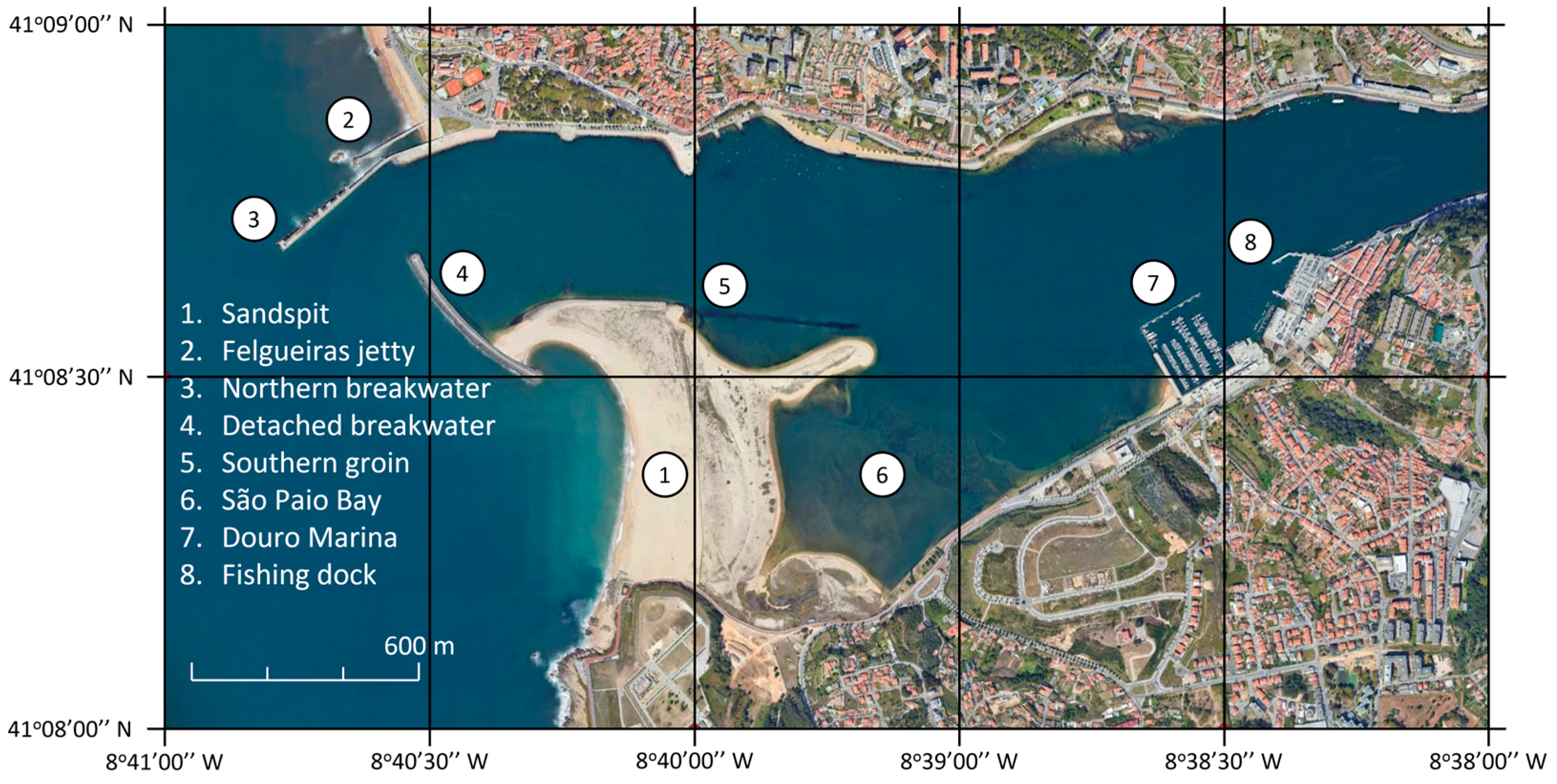
Figure 2.
(a) Significant (●●●) and maximum (●●●) wave heights recorded at the Leixões wave buoy (time referred to 00h00 UTC 6 January 2014). (b) Ascending zero-crossing (●●●) and maximum (●●●) wave periods recorded at the Leixões wave buoy (time referred to 00h00 UTC 6 January 2014).
Figure 2.
(a) Significant (●●●) and maximum (●●●) wave heights recorded at the Leixões wave buoy (time referred to 00h00 UTC 6 January 2014). (b) Ascending zero-crossing (●●●) and maximum (●●●) wave periods recorded at the Leixões wave buoy (time referred to 00h00 UTC 6 January 2014).
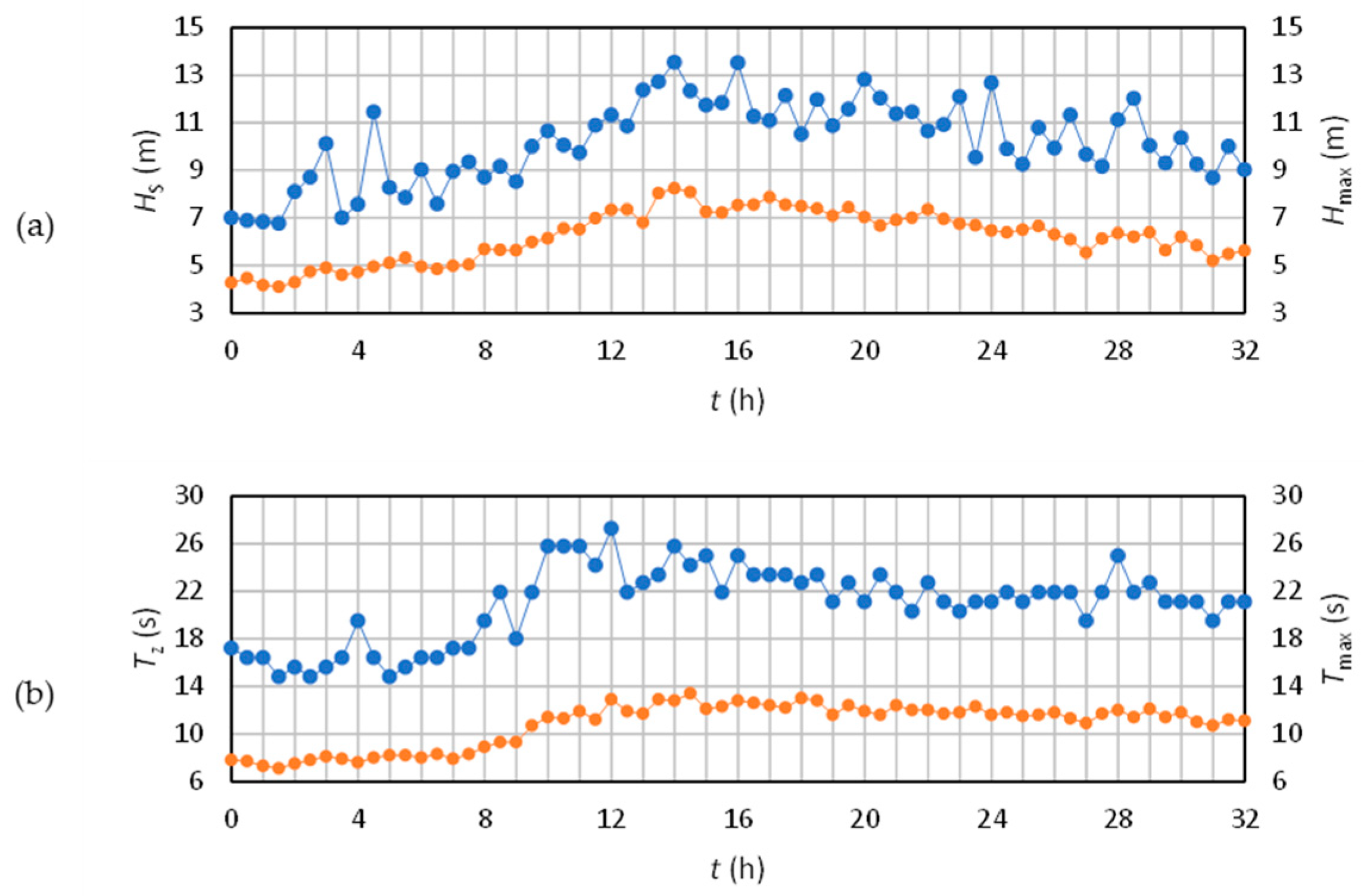
Figure 3.
(a) Boundaries and bathymetry of model M1, Ibero-Atlantic regional model (▬), and location of model M2 (▬); horizontal datum: WGS84 (epsg:4326), vertical datum: mean sea level (MSL) in 2021. (b) Boundaries and bathymetry of model M2, Espinho-Lavra coastal model (▬), and location of model M3 (▬); horizontal datum: WGS84 (epsg:4326), vertical datum: MSL in 2021. (c) Computational domain and topobathymetry of the Foz do Douro local model M3; horizontal datum: ETRS89/PT-TM06 (epsg:3763), vertical datum: Cascais 1938 (epsg:5780), corresponding to the adopted mean sea level (NMM).
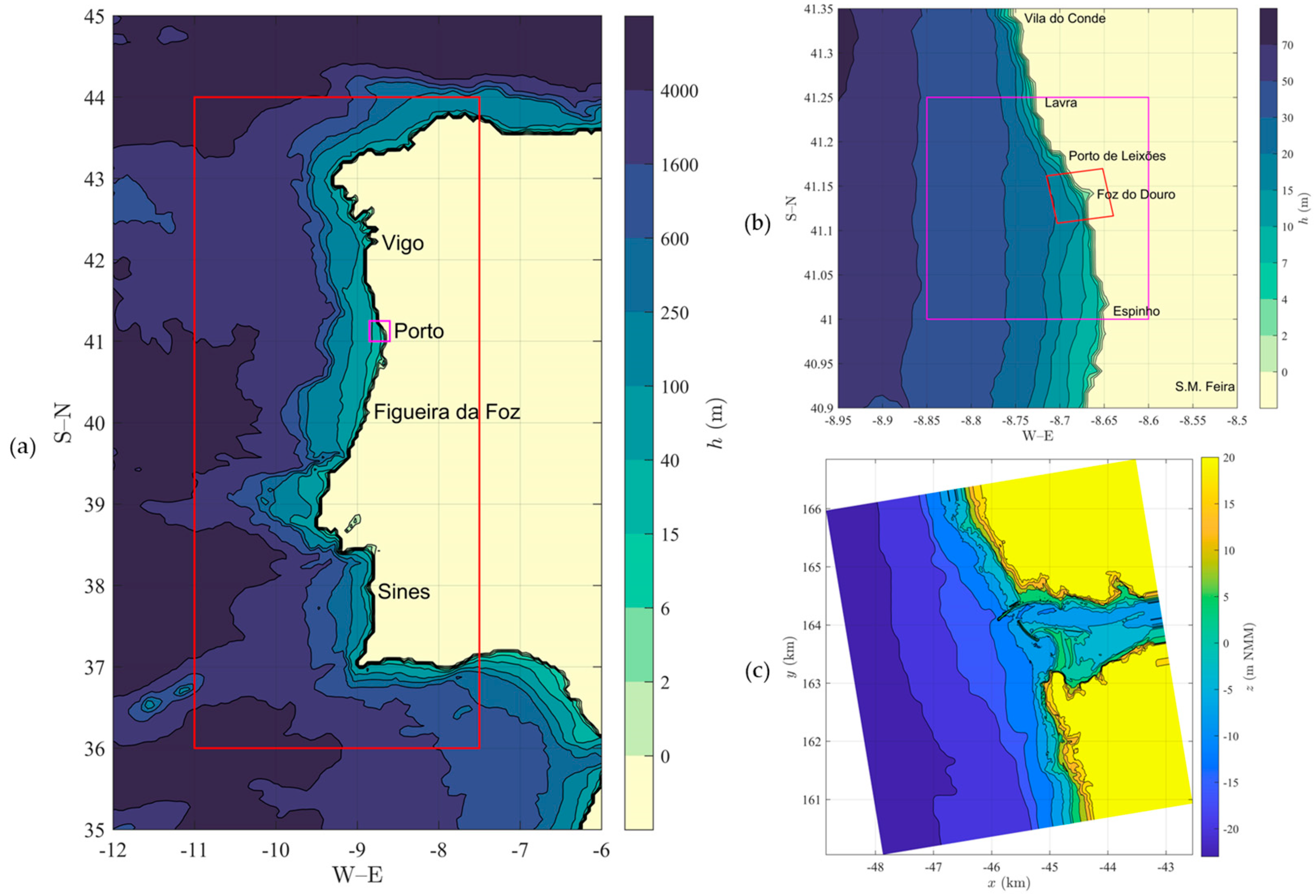
Figure 4.
Comparison of the observed (o) and synthetic (—) water level time series at Viana do Castelo (time referred to 00h00 UTC on 1 August 2014). For clarity, only the first two weeks are shown.
Figure 4.
Comparison of the observed (o) and synthetic (—) water level time series at Viana do Castelo (time referred to 00h00 UTC on 1 August 2014). For clarity, only the first two weeks are shown.
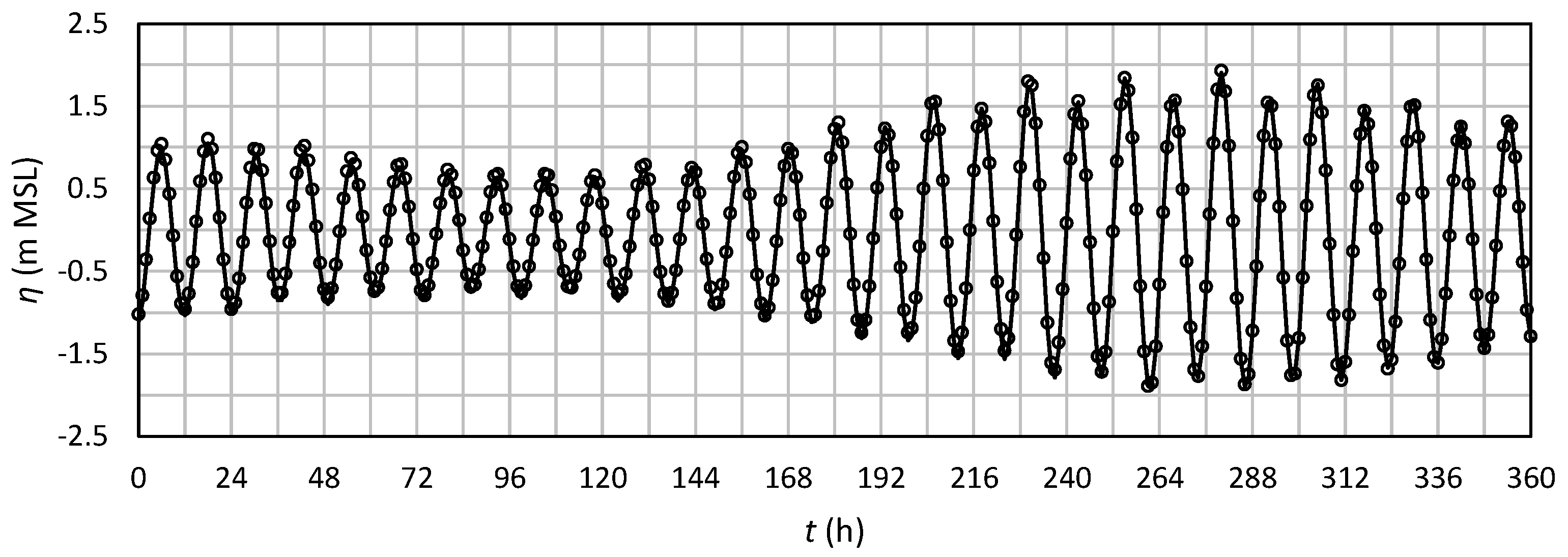
Figure 5.
Detail of the initial topobathymetry of the Douro estuary and river mouth and location of transects 1–4 (details about the data sources used are given in Section 2.1).
Figure 5.
Detail of the initial topobathymetry of the Douro estuary and river mouth and location of transects 1–4 (details about the data sources used are given in Section 2.1).

Figure 6.
Time-averaged significant wave height in the period 18h00–21h00 UTC on 6 January 2014, for scenarios S1 and S7.
Figure 6.
Time-averaged significant wave height in the period 18h00–21h00 UTC on 6 January 2014, for scenarios S1 and S7.
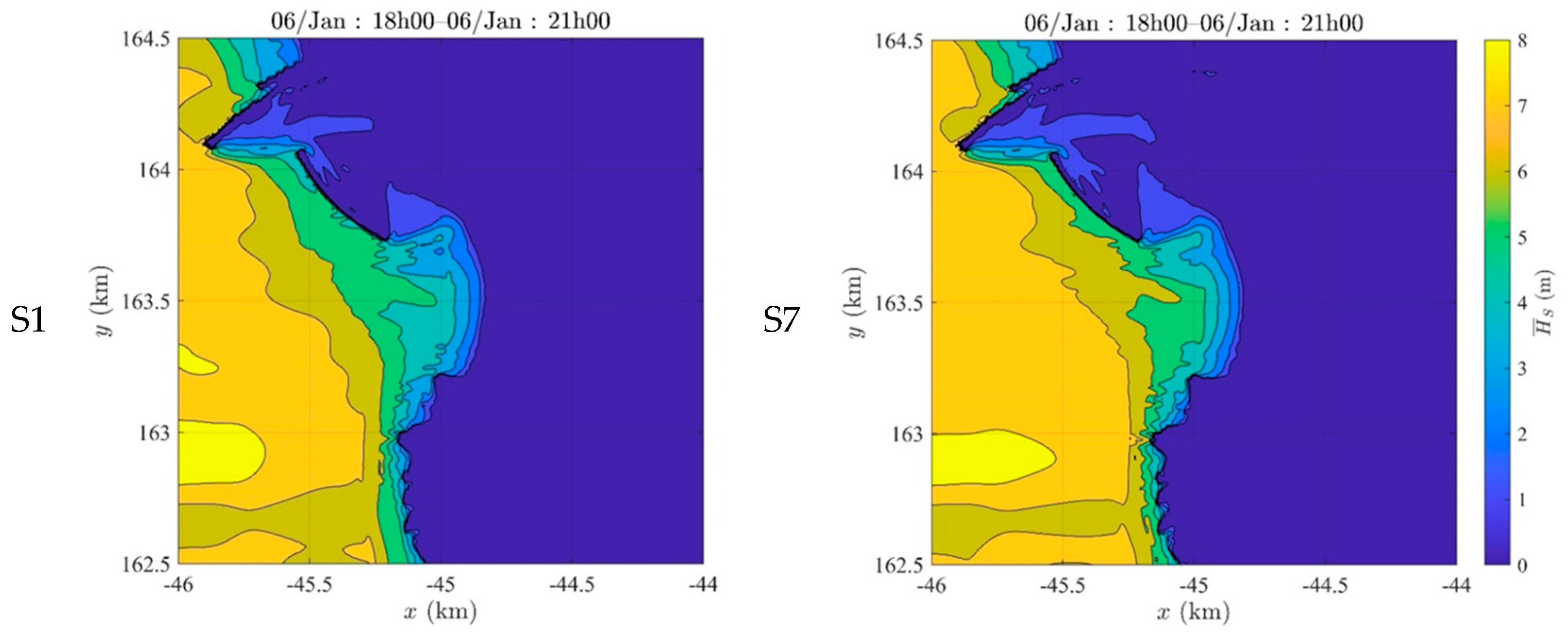
Figure 7.
Scenario S1. Extreme (maximum and minimum) and mean sea level for (a) transect 1, (b) transect 2, (c) transect 3 (W–E direction), and (d) transect 4 (S–N direction).
Figure 7.
Scenario S1. Extreme (maximum and minimum) and mean sea level for (a) transect 1, (b) transect 2, (c) transect 3 (W–E direction), and (d) transect 4 (S–N direction).

Figure 8.
Scenario S7. Extreme (maximum and minimum) and mean sea level for (a) transect 1, (b) transect 2, (c) transect 3 (W–E direction), and (d) transect 4 (S–N direction).
Figure 8.
Scenario S7. Extreme (maximum and minimum) and mean sea level for (a) transect 1, (b) transect 2, (c) transect 3 (W–E direction), and (d) transect 4 (S–N direction).
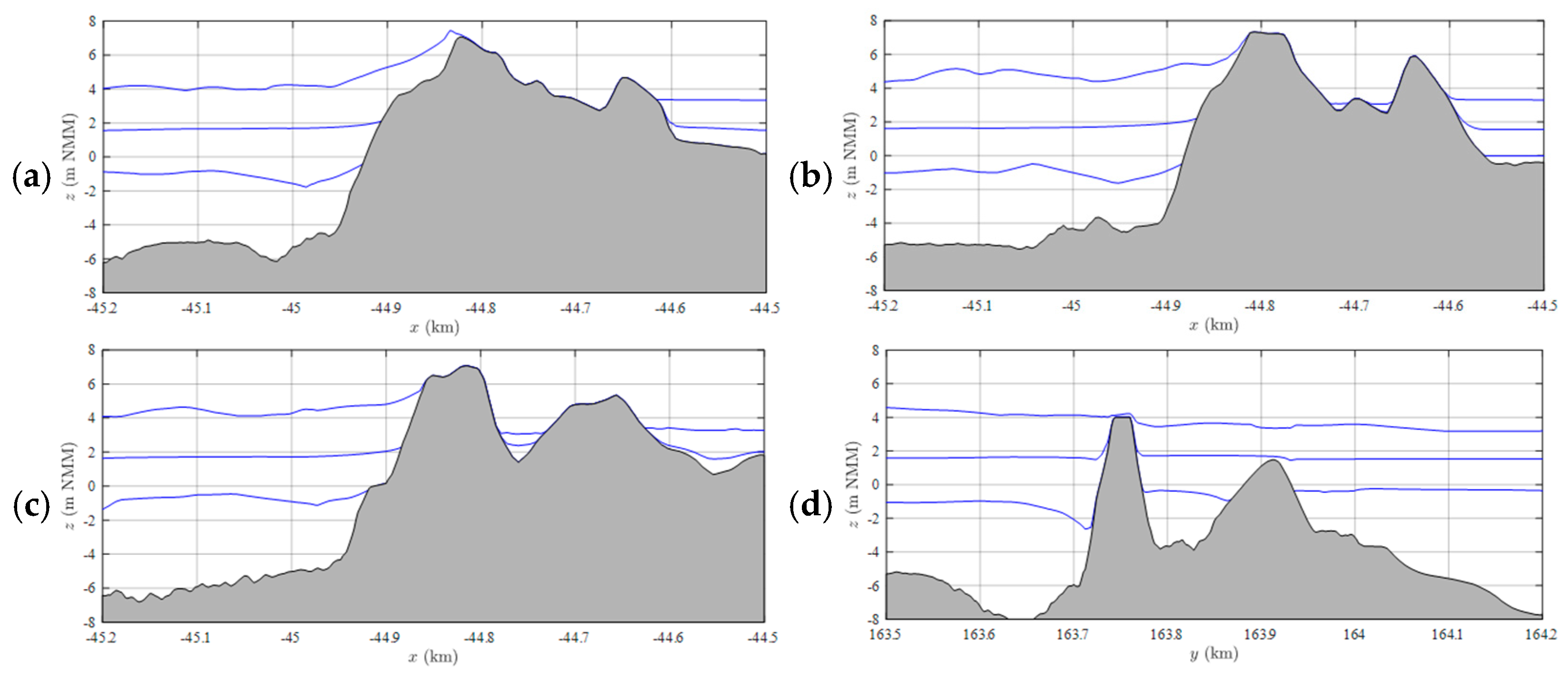
Figure 9.
Erosion and accretion of the sandspit at 00h00 UTC on 8 January 2014 for scenarios S1 and S7.
Figure 9.
Erosion and accretion of the sandspit at 00h00 UTC on 8 January 2014 for scenarios S1 and S7.

Figure 10.
Scenario S1. Evolution of topobathymetric profiles for (a) transect 1, (b) transect 2, (c) transect 3 (W–E direction), and (d) transect 4 (S–N direction).
Figure 10.
Scenario S1. Evolution of topobathymetric profiles for (a) transect 1, (b) transect 2, (c) transect 3 (W–E direction), and (d) transect 4 (S–N direction).

Figure 11.
Scenario S7. Evolution of topobathymetric profiles for (a) transect 1, (b) transect 2, (c) transect 3 (W–E direction), and (d) transect 4 (S–N direction).
Figure 11.
Scenario S7. Evolution of topobathymetric profiles for (a) transect 1, (b) transect 2, (c) transect 3 (W–E direction), and (d) transect 4 (S–N direction).


Table 1.
Boundary conditions and physical processes for the calibration of model M1.
| Boundary Conditions | Physical Processes | ||||||
|---|---|---|---|---|---|---|---|
| ECMWF | CMEMS-IBI | Friction | Linear Growth | Exponential Growth | Whitecapping | Wind Drag | |
| T01 | ✓ | JONSWAP | Activated | Komen | Komen | Fit | |
| T02 | ✓ | JONSWAP | Activated | Komen | Janssen | Fit | |
| T03 | ✓ | JONSWAP | Activated | Komen | Komen | Wu | |
| T04 | ✓ | JONSWAP | Activated | Rogers/Babanin | Rogers/Babanin | Hwang | |
| T05 | ✓ | JONSWAP | Activated | Komen | Komen | Fit | |
| T06 | ✓ | JONSWAP | Activated | Westhhuysen/Yan | Alves-Banner | Fit | |
Table 2.
Spectral parameter metrics for SWAN configurations.
| T01 | T02 | T03 | T04 | T05 | T06 | |||
|---|---|---|---|---|---|---|---|---|
| (m) | 0.580 | 0.625 | 0.567 | 0.492 | 0.456 | 0.440 | ||
| (—) | 0.147 | 0.159 | 0.144 | 0.125 | 0.116 | 0.112 | ||
| (m) | −0.336 | −0.392 | −0.315 | −0.182 | 0.031 | −0.020 | ||
| (—) | 0.894 | 0.880 | 0.899 | 0.937 | 0.990 | 0.989 | ||
| (—) | 0.960 | 0.957 | 0.959 | 0.956 | 0.955 | 0.957 | ||
| (s) | 0.999 | 0.958 | 0.931 | 0.593 | 1.950 | 1.594 | ||
| (—) | 0.113 | 0.108 | 0.105 | 0.067 | 0.221 | 0.180 | ||
| (s) | 0.692 | 0.609 | 0.600 | −0.038 | 1.769 | 1.451 | ||
| (—) | 1.084 | 1.075 | 1.073 | 0.996 | 1.207 | 1.165 | ||
| (—) | 0.933 | 0.933 | 0.936 | 0.936 | 0.936 | 0.930 | ||
| (s) | 0.765 | 0.789 | 0.779 | 1.348 | 1.281 | 0.711 | ||
| (—) | 0.087 | 0.089 | 0.088 | 0.153 | 0.145 | 0.080 | ||
| (s) | 0.009 | −0.114 | −0.129 | −1.203 | 0.626 | −0.291 | ||
| (—) | 1.009 | 0.995 | 0.993 | 0.861 | 1.085 | 0.967 | ||
| (—) | 0.926 | 0.922 | 0.924 | 0.932 | 0.891 | 0.920 | ||
| (1) | (°N) | 21.31 | 21.53 | 20.52 | 20.60 | 21.75 | 22.00 | |
| (°N) | 7.64 | 6.93 | 7.44 | 7.47 | 9.05 | 8.99 | ||
| (—) | 0.661 | 0.672 | 0.698 | 0.693 | 0.603 | 0.586 |
Note(s): 1 Nautical convention.
Table 3.
Sea level rise simulation scenarios.
| Scenario | Year | ||||
|---|---|---|---|---|---|
| (%) | (m MSL) | (m NMM) | |||
| S1 | Historical | 2021 | 0.000 | 0.221 | |
| S2 | SSP2-4.5 | 2100 | 5 | 0.253 | 0.480 |
| S3 | SSP2-4.5 | 2100 | 50 | 0.473 | 0.753 |
| S4 | SSP2-4.5 | 2100 | 95 | 0.867 | 1.206 |
| S5 | SSP5-8.5 | 2100 | 5 | 0.424 | 0.651 |
| S6 | SSP5-8.5 | 2100 | 50 | 0.784 | 0.949 |
| S7 | SSP5-8.5 | 2100 | 95 | 1.391 | 1.502 |
Table 4.
Model metrics for the Leixões buoy data for the period 1–15 January 2014.
| (m, s, °) | (—) | (m, s, °) | (—) | (—) | |
|---|---|---|---|---|---|
| 0.447 | 0.093 | −0.171 | 0.958 | 0.957 | |
| 1.319 | 0.094 | 0.593 | 1.006 | 0.764 | |
| 0.667 | 0.074 | 0.149 | 0.997 | 0.911 | |
| 8.744 | −0.182 | 0.937 | 0.613 |
Table 5.
Erosion/accretion in the sandspit (for the area represented in Figure 9).
Table 5.
Erosion/accretion in the sandspit (for the area represented in Figure 9).
| Scenario | Volume | Area | ||||||
|---|---|---|---|---|---|---|---|---|
| Accretion | Erosion | Budget | Accretion | Erosion | ||||
| (%) | (m NMM) | (m3) | (m3) | (m3) | (%) | (%) | ||
| S1 | Historical | 0.221 | 187,862 | 193,761 | −5899 | 44 | 35 | |
| S2 | SSP2-4.5 | 5 | 0.480 | 196,804 | 201,908 | −5104 | 45 | 35 |
| S3 | SSP2-4.5 | 50 | 0.753 | 198,131 | 196,242 | +1889 | 48 | 34 |
| S4 | SSP2-4.5 | 95 | 1.206 | 217,982 | 211,624 | +6358 | 51 | 33 |
| S5 | SSP5-8.5 | 5 | 0.651 | 208,310 | 214,428 | −6117 | 45 | 36 |
| S6 | SSP5-8.5 | 50 | 0.949 | 216,886 | 209,653 | +7233 | 48 | 33 |
| S7 | SSP5-8.5 | 95 | 1.502 | 239,407 | 239,354 | +53 | 54 | 34 |
Disclaimer/Publisher’s Note: The statements, opinions and data contained in all publications are solely those of the individual author(s) and contributor(s) and not of MDPI and/or the editor(s). MDPI and/or the editor(s) disclaim responsibility for any injury to people or property resulting from any ideas, methods, instructions or products referred to in the content. |
© 2023 by the authors. Licensee MDPI, Basel, Switzerland. This article is an open access article distributed under the terms and conditions of the Creative Commons Attribution (CC BY) license (https://creativecommons.org/licenses/by/4.0/).
Share and Cite
MDPI and ACS Style
Caeiro-Gonçalves, F.; Bio, A.; Iglesias, I.; Avilez-Valente, P. Sea Level Rise Effects on the Sedimentary Dynamics of the Douro Estuary Sandspit (Portugal). Water 2023, 15, 2841. https://doi.org/10.3390/w15152841
AMA Style
Caeiro-Gonçalves F, Bio A, Iglesias I, Avilez-Valente P. Sea Level Rise Effects on the Sedimentary Dynamics of the Douro Estuary Sandspit (Portugal). Water. 2023; 15(15):2841. https://doi.org/10.3390/w15152841
Chicago/Turabian StyleCaeiro-Gonçalves, Francisca, Ana Bio, Isabel Iglesias, and Paulo Avilez-Valente. 2023. "Sea Level Rise Effects on the Sedimentary Dynamics of the Douro Estuary Sandspit (Portugal)" Water 15, no. 15: 2841. https://doi.org/10.3390/w15152841
Note that from the first issue of 2016, this journal uses article numbers instead of page numbers. See further details here.