Abstract
The likelihood of surface water and groundwater contamination is higher in regions close to landfills due to the possibility of leachate percolation, which is a potential source of pollution. Therefore, proposing a reliable framework for monitoring leachate and groundwater parameters is an essential task for the managers and authorities of water quality control. For this purpose, an efficient hybrid artificial intelligence model based on grey wolf metaheuristic optimization algorithm and extreme learning machine (ELM-GWO) is used for predicting landfill leachate quality (COD and BOD5) and groundwater quality (turbidity and EC) at the Saravan landfill, Rasht, Iran. In this study, leachate and groundwater samples were collected from the Saravan landfill and monitoring wells. Moreover, the concentration of different physico-chemical parameters and heavy metal concentration in leachate (Cd, Cr, Cu, Fe, Ni, Pb, Mn, Zn, turbidity, Ca, Na, NO3, Cl, K, COD, and BOD5) and in groundwater (Cd, Cr, Cu, Fe, Ni, Pb, Mn, Zn, turbidity, EC, TDS, pH, Cl, Na, NO3, and K). The results obtained from ELM-GWO were compared with four different artificial intelligence models: multivariate adaptive regression splines (MARS), extreme learning machine (ELM), multilayer perceptron artificial neural network (MLPANN), and multilayer perceptron artificial neural network integrated with grey wolf metaheuristic optimization algorithm (MLPANN-GWO). The results of this study confirm that ELM-GWO considerably enhanced the predictive performance of the MLPANN-GWO, ELM, MLPANN, and MARS models in terms of the root-mean-square error, respectively, by 43.07%, 73.88%, 74.5%, and 88.55% for COD; 23.91%, 59.31%, 62.85%, and 77.71% for BOD5; 14.08%, 47.86%, 53.43%, and 57.04% for turbidity; and 38.57%, 59.64%, 67.94%, and 74.76% for EC. Therefore, ELM-GWO can be applied as a robust approach for investigating leachate and groundwater quality parameters in different landfill sites.
1. Introduction
Landfill sites play a crucial role in safeguarding the environment. The process of treating leachate holds significant importance in the functioning of landfill sites. Accurately predicting the volume and composition of leachate relies heavily on climate conditions and the types of waste materials being disposed of, making them pivotal factors in minimizing the environmental impact on the surrounding area during landfill operations. Serious environmental damage may occur due to waste burial in uncontrolled landfills. As a consequence of this, landfill-based leachates have a high potential for the contamination of soil and groundwater resources. The management of leachate and the prediction of its quality and quantity are essential because of its considerable environmental impacts. Without a proper design of landfills, leachate can spread in the environment and, hence, leachate monitoring is necessary for engineered landfills. Providing an accurate prediction method for analyzing leachate quantity/quality can considerably reduce the high cost of monitoring programs [1,2].
Many prediction models based on water balance in landfill sites are used for analyzing the quantity and quality of leachate. These involve the hydrologic assessment of a landfill model [2,3,4,5], which is the equation of Richard for one-phase unsaturated flow through homogeneous and heterogeneous porous media [6,7,8]. Another method used for analyzing solute transport in landfills is a convective–dispersive equation, which uses the transport and transformation processes of dispersion, advection, and sorption in unsaturated porous media and chemical and biological transformation [9,10,11,12]. The main disadvantage of such models is the fact that they require a high number of parameters based on chemical, hydraulic, and biological characteristics. Additionally, mechanical properties are identified utilizing optimization methods considering measured values in an objective landfill site [13]. Since such models are very complicated, they cannot be applied in the actual operation of landfill sites. However, they are useful for optimizing the landfill sites’ performance [2]. Due to the limitations mentioned above, researchers have turned to machine learning (ML) methods as a viable solution for intricate nonlinear hydrological modeling. The reason behind this shift is ML’s capability to handle vast quantities of data efficiently [14].
In recent decades, machine learning models have been successfully used for modeling environmental phenomena. However, there is limited number of studies that investigate the efficiency of ML models in analyzing landfill leachate quantity/quality based on chemical oxygen demand (COD), biochemical oxygen demand (BOD5), turbidity, and electrical conductivity (EC) of leachate and groundwater quality parameters. These include COD prediction in leachate using multi-layer perceptron neural networks (MLPANNs) and M5 model tree to simulate the Khulna landfill in Bangladesh [1], the prediction of temporal variations in the leachate COD concentration using MLPANN [15,16], and the prediction of COD using MLPANN and the response surface method (RSM) for the treatment of landfill leachate [17]. Bhatt et al. (2016) used multi-linear regression for estimating COD and BOD5 concentrations of conventional municipal solid waste landfill considering the inputs of precipitation rate, temperature, and different types of waste percentages [18]. Bhatt et al. (2017) estimated leachate BOD5 and COD obtained from a laboratory using multivariate adaptive regression spline (MARS). They reported the usefulness of this method in the prediction of leachate quality parameters using waste composition, temperature, and rainfall rate information [19]. According to the authors’ knowledge, two-stage MLPANN and extreme learning machine (ELM) integrated with grey wolf metaheuristic optimization have not been used for analyzing landfill leachate quality based on COD and BOD5 concentrations before.
Due to its better prediction efficiency and less time consumption compared to other conventional ML models, ELM has been widely used for solving problems in different engineering fields [20,21,22,23]. However, since the single ELM model randomly initializes its hyper-parameters, this may cause an overfitting problem and affect the predictive performance seriously. To cope with this disadvantage, advanced metaheuristic optimization algorithms, such as GWO, are required. GWO is one of the modern bio-inspired algorithms commonly utilized for improving ML models [24]. Compared to other bio-inspired intelligent optimization algorithms, the advantages of GWO are: (i) it has no tuned parameters, (ii) its implementation and adaptation to the optimization problems are easy, and (iii) it has more flexibility and scalability [25]. Additionally, the modeling, prediction, and forecasting of groundwater quantity and quality employing ML models and metaheuristic optimization algorithms have been reported. Ghobadi et al. (2022) enhanced the precision of estimating water quality parameters, such as total dissolved solids (TDS), dissolved oxygen (DO), and turbidity, using the MLPANN model. The research was conducted in the Asadabad Plain, Iran, and involved a comparison with standard MLPANN, generalized regression neural network (GRNN), and multiple linear regression (MLR) methods. The findings indicated that the hybrid GWO-MLPANN approach proved to be a valuable tool for estimating water quality, demonstrating a high accuracy and performance [26]. Fadhillah et al. (2021) employed the GWO technique to enhance the performance of support vector machine (SVM) in mapping groundwater potential in Gangneungsi, South Korea. By applying the GWO algorithm, the accuracy of the SVM model was improved by 8.6% [27]. Moayedi et al. (2023) assessed the precision of three ML paradigms, namely grey wolf optimization (GWO), artificial bee colony (ABC), and Harris hawks Optimization (HHO) intelligence models, in predicting the total hardness of groundwater quality in the Shiraz Plain, Iran. The results demonstrated that the GWO-ANN approach exhibited a high accuracy and capability in simulating and evaluating the quality of groundwater [28]. Nordin et al. (2021) reviewed four ML models for groundwater quality field. They found that an artificial neural network (ANN) showed a better performance in controlling a large dataset and providing accurate predictions [14].
COD and BOD5 are among the most important indicators for the pollutants that leach from landfills [29]. The novelty of the presented study lies in its investigation of the applicability of two hybrid models, namely MLPANN and ELM integrated with GWO, for accurately predicting COD and BOD5 in order to assess and analyze landfill leachate quality. This approach has not been previously explored in the specific context of landfill leachate analysis based on COD and BOD5 parameters. Additionally, the study extends its analysis to predict groundwater quality in terms of turbidity and electrical conductivity parameters using the same hybrid models. By comparing the results of the hybrid models with single MLPANN, ELM, and tree-based MARS models, the study contributes to understanding the advantages and performance of the proposed approach in accurately assessing landfill leachate and groundwater quality.
2. Data and Methods
2.1. Study Area, Leachate, and Groundwater Data
In this study, the Saravan landfill in the north of Iran was selected as the case study to investigate leachate and groundwater quality by using different artificial intelligence models, including MARS, MLPANN, ELM, MLPANN-GWO, and ELM-GWO. The groundwater in this area is the main resource for drinking and agriculture purposes. In this research, two series data were gathered from both leachate quality (30 data points) parameters (Cd, Cr, Cu, Fe, Ni, Pb, Mn, Zn, turbidity, Ca, Na, NO3, Cl, K, COD, and BOD5) and groundwater quality (30 data points) parameters (Cd, Cr, Cu, Fe, Ni, Pb, Mn, Zn, turbidity, EC, TDS, pH, Cl, Na, NO3, and K) from five different monitored wells to predict leachate quality (COD and BOD5) and groundwater quality (turbidity and EC) as the target parameters. The Saravan landfill (latitude 37°4′17.94″ N, longitude 49°37′52:70″ E), which has an altitude of 200 m above sea level, is located 20 km away from Rasht city and has a mild and humid climate condition. The average annual rainfall in the region is 1300 mm, the average temperature is 15.9 °C, and the relative humidity is about 81.9%. The geographical location of landfill is shown in Figure 1.
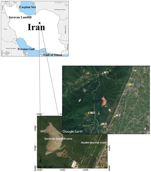
Figure 1.
Location map of the study area and groundwater monitoring wells (W1, W2, W3, W4, and W5).
2.2. Artificial Intelligence Methods
2.2.1. Multivariate Adaptive Regression Splines (MARS)
Multivariate adaptive regression splines (MARS) was introduced by Friedman (1991) [30]. MARS is a modelling strategy mainly used for expressing the relationship between an ensemble of input variables and their corresponding output variable, i.e., the variable to be modeled (Figure 2). The mathematical formulation of the MARS model can be established in the form of basis function (BFs) with an ensemble of parameters determined during the training stage. The nonlinear function f(X) linking the input to the output variables can be expressed using MARS model as follows [31,32,33,34,35]:
where f(X) is the MARS predictor; X corresponds to the input variables; are the coefficients obtained using the least squared method; is the mth basis function, which can be a single spline or an interaction of several spline functions (i.e., one or more); M is the number of basis function; and is the coefficient of the constant basis function. For solving any regression problem using MARS, a three-step model is needed. First, we start with a constructive phase; a global model composed of a large number of BF is constructed. These basis functions are introduced in several regions of the input variables, and they are combined, which can lead to the overfitting of the model. Consequently, the second step is reserved for the pruning of the model by deleting some of that irrelevant BF. Finally, in the third step, the model is fixed using only a sequence of sampler BF [32,33,34].
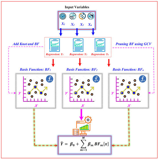
Figure 2.
The multivariate adaptive regression splines (MARS) structure.
2.2.2. Extreme Learning Machine (ELM)
Extreme learning machine (ELM) [36,37] was originally proposed for fast training the single-hidden layer feedforward neural networks (SLFNs). Using the ELM model, the hidden neurons’ parameters, i.e., the weights and biases (Wij, bj), were randomly generated and they do not need to be tuned, while the output parameters, i.e., the βj, were analytically computed (Figure 3). The ELM mathematical formulation can be written as follows:
where wi and bi are the weights and biases of the hidden nodes, respectively, and βi is the weight connecting the ith hidden neuron to the output neuron. is the output of the ith hidden neuron, and G is the activation function. For any set of training sample data, . For an ideal model having the output equal exactly to the target data, the following expression can be written [38,39,40]:
where:
where, H is the hidden-layer output matrix of the network. β and T are the corresponding matrices of output weights and targets. So, the output matrix β can be estimated analytically by:
where H+ is the Moore–Penrose generalized inverse of H [40,41,42].
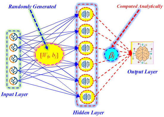
Figure 3.
The extreme learning machine structure.
2.2.3. Multilayer Perceptron Artificial Neural Network (MLPANN)
The multilayer perceptron artificial neural network (MLPANN) is a kind of machine learning model used for the estimation of an output variable, Y, for given input variables, X, such as Y = f(X) for a given function f (.) [43]. The MLPANN can be defined as a mathematical model composed from a number of highly interconnected processing elements organized into several layers similar to that of the human brain [44]. The MLPANN provides a decision based on the information acquired during previous experiments. According to Figure 4, the MLPANN is composed of one input layer, one hidden layer, and one output layer. The neurons in each layer play a particular role. By the end of the data preprocessing, the available information is spread to all the following layers with lightning speed, thus from the input to the hidden and from the hidden to the output layers. The neurons of the input layer are used only for the presentation of the variables to the model, while the hidden neurons play a major and critical role in the model structure, and they are equipped by a nonlinear sigmoidal activation function [45]. The final response of the model is then provided by the single output neuron equipped by a linear activation function. The parameters of the MLPANN model are the weights and biases, and they are updated during the training process [46]. For any developed MLPANN model, dataset should be divided into two subsets; the first, generally equal to 70%, is used for training the network and providing the final parameters and biases, while the remaining 30% are used for testing the generalization capability of the model [47,48].
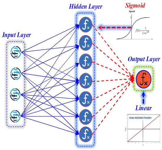
Figure 4.
The multilayer perceptron neural network structure.
2.2.4. Grey Wolf Optimization (GWO)
The grey wolf optimization (GWO) metaheuristic algorithm was proposed by Mirjalili et al. (2014) [24]. GWO belongs to the category of swarm-based optimization algorithms and it was inspired by the hierarchy observed among grey wolves (GWs). In this algorithm, there exist four categories of wolves, which are alpha (α), beta (β), delta (δ), and omega (ω) (Figure 5). According to [24], GWO is composed of three main steps: (i) encircling the prey, (ii) hunting, and (iii) attacking the prey or the exploitation phase. The GWO algorithm can be expressed as follows.
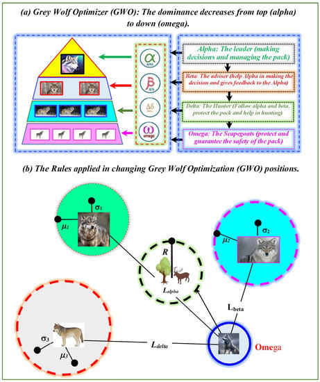
Figure 5.
The gray wolf optimization algorithm (GWO) diagram [24].
The encircling prey (Ry) is the stage during which the GW encircles the prey and it can be written as follows [24]:
In Equations (7) and (8), there are two important positions: shows the position of the prey and is the position of the grey wolf. and are coefficient vectors and (t) is the current iteration. and can be calculated as follows:
where decreases from two to zero, while and are random vectors in the interval of [0, 1]. It has been shown that omegas follow the best search agents, i.e., α, β, and δ, and their positions are continuously saved as follows (Figure 6):
where , , and are the current positions of the alpha, beta, and delta wolves. This stage of the algorithm, i.e., the attack of the prey, can be expressed by changing the value of through decreasing levels and consequently the value of [24]. Figure 6 shows the flowchart of GWO.
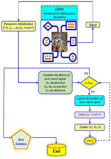
Figure 6.
Flowchart of the grey wolf optimization algorithm.
2.2.5. Hybrid Models Based on the Grey Wolf Optimization Algorithm
In the present study, five different machine learning models (MARS, MLPANN, ELM, MLPANN-GWO, and ELM-GWO) were applied and compared. The GWO algorithm was used to find the most efficient model parameters, which can effectively improve the prediction performances of the ML models in predicting leachate and groundwater quality parameters. For the ELM, GWO was used for the optimization of the hidden neuron parameters, i.e., the weight and biases, taking into account the cost function, i.e., the RMSE. Similarly, for the MLPANN model, the weight and biases of the model were considered as parameters that should be optimized by updating the grey wolves’ location information, i.e., Z(t), consequently updating the location that can lead to finding the optimum values of the weight and biases. It is worth mentioning that the GWO algorithm parameters were set as follows:
- Fitness function = Root-mean-square error.
- Iterations number = 200.
- Number of agents = 100.
- C = random vector in [0, 2].
- a = in every iteration, this parameter is lowered from 2 to 0.
- A = [−a, a].
3. Model Performance Evaluation Metrics
To examine the performance of the MARS, MLPANN, ELM, MLPANN-GWO, and ELM-GWO models for the prediction of landfill leachate and groundwater quality, four statistical measures, including root-mean-square error (RMSE), Nash–Sutcliffe efficiency (NS), mean absolute error (MAE), and correlation coefficient (R), were utilized. The following equations can be applied to calculate the mentioned metrics:
where represents the models’ generated results and indicates the observed values for the leachate and groundwater quality parameters. Additionally, n shows the total number of data points.
4. Results
In the current research procedure, two case studies (leachate and groundwater quality modeling) were adopted utilizing the individual water quality parameters (i.e., COD, BOD5, turbidity, and EC) in the Saravan landfill, which has five groundwater monitoring wells, in Iran. Assigning the sufficient approach of input combinations for individual water quality parameters, a different decision regarding the input variables was reached for the diverse input combinations in both case studies.
First, COD and BOD5 concentrations were predicted based on different machine learning (ML) models, including MARS, MLPANN, ELM, MLPANN-GWO, and ELM-GWO, for the leachate quality assessment. In the case of the COD parameter, Na, NO3, K, Cu, Cd, Cr, and Fe were used as the input variables, whereas the input variables of the BOD5 parameter were Ca, Na, NO3, Cu, Zn, Cr, Ni, and Fe. Second, the values of the turbidity and EC indicators were predicted utilizing the afore-mentioned ML models for groundwater quality assessment. The turbidity indicator was predicted based on the combination of Cl, pH, K, Cr, Zn, Fe, Mn, and Cu, while the predictive procedure of the EC indicator was conducted in conjunction with Cl, Na, K, Cr, Pb, Zn, Mn, Ni, and Cu.
As explained in the previous section, the evaluation of single-stage (i.e., MARS, MLPANN, and ELM) and two-stage (i.e., metaheuristic optimization algorithm integrated with machine learning, MLPANN-GWO and ELM-GWO) models for predicting concentrations (COD and BOD5) and values (turbidity and EC) is the critical feature of the current research.
4.1. Predicting COD and BOD5 Concentrations in the Leachate Quality of the Saravan Landfill
4.1.1. Application of Single- and Two-Stage ML Models for COD Concentration
The predictive results of single- and two-stage ML models utilizing four statistical measures (i.e., RMSE, NS, R, and MAE) for COD concentration is shown in Table 1. Additionally, it shows that the predictive results of the ELM-GWO (RMSE = 21.12 mg/L, NS = 0.998, and MAE = 17.43 mg/L) model was superior to those of the MARS, MLPANN, ELM, and MLPANN-GWO models in the leachate quality of the Saravan landfill during the testing phase.

Table 1.
Testing results of the applied models for predicting the COD concentration in leachate quality assessment.
Figure 7a–e show the scatter plots of the observed and predicted COD concentration for single- and two-stage ML models. The blue color of the line, equal line, and R values are situated clearly in the corresponding scatter plots. It can be observed from Figure 7a–e that there is a clear difference between the single- and two-stage ML models. Additionally, the ELM-GWO model supplied the first-rate R value (R = 0.999) between single- and two-stage ML models.
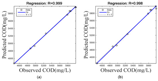
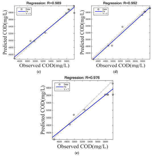
Figure 7.
Scatter plots of the observed and predicted COD concentrations for the single- and two-stage ML models: (a) ELM-GWO, (b) MLPANN-GWO, (c) ELM, (d) MLPANN, and (e) MARS.
Supplementary information can assess the achievement of single- and two-stage ML models utilizing a Taylor diagram [49] and violin plot [50]. The Taylor diagram (Figure 8) applies three specific statistical measures, such as root-mean-square error, normalized standard deviation, and correlation coefficient, for plotting the observed and predicted COD concentrations. The Taylor diagram can be used to detect the most adjacent model with the predicted COD concentration conditional on the correlation coefficient (radial axis) and standard deviation (polar axis). Figure 8, therefore, illustrates the real precision of the ELM-GWO model for predicting the COD concentration compared to other single- and two-stage ML models.
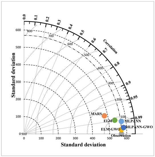
Figure 8.
Taylor diagram of the observed and predicted COD concentrations for single- and two-stage ML models.
The violin plot can be used as one of approaches to confirm the allocation of the described numerical values. Figure 9 presents the comparable structures of the ELM-GWO, MLPANN-GWO, and ELM models following the observed values of the COD concentration, including the maximum, minimum, mean, and median, based on single- and two-stage ML models in the leachate quality of the Saravan landfill.
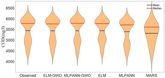
Figure 9.
Violin plot of the observed and predicted COD concentrations for single- and two-stage ML models.
4.1.2. Application of Single- and Two-Stage ML Models for BOD5 Concentration
The predictive assessment of single- and two-stage ML models dependent on four statistical measures (RMSE, NS, R, and MAE) for BOD5 concentration is presented in Table 2. It shows that the predictive results of the ELM-GWO (RMSE = 10.50 mg/L, NS = 0.996, and MAE = 9.21 mg/L) model were better compared to the different models, including MARS, MLPANN, ELM, and MLPANN-GWO, in the leachate quality of the Saravan landfill during the testing phase.
Table 2.
Testing results of the applied models for predicting BOD5 concentration in leachate quality assessment.
Figure 10a–e present the scatter plots of the observed and predicted BOD5 concentrations for single- and two-stage ML models. The correlation coefficient (R) value, dotted (equal) line, and blue color (fitted) line are observed in the independent scatter plots. It can be observed from Figure 10a–e that an apparent discrepancy is present between the single- and two-stage ML models. That is, the ELM-GWO model had the best R value (R = 0.999) between the single- and two-stage ML models.
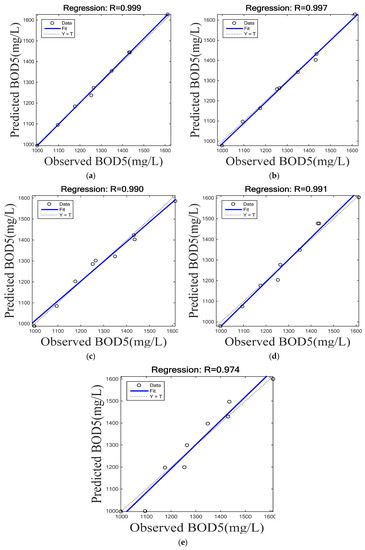
Figure 10.
Scatter plots of the observed and predicted BOD5 concentrations for single- and two-stage ML models: (a) ELM-GWO, (b) MLPANN-GWO, (c) ELM, (d) MLPANN, and (e) MARS.
Additionally, since the ELM-GWO model is located very close to the observed BOD5 concentration, it can be inferred from the Taylor diagram (Figure 11) that the ELM-GWM model provides a reliable performance for predicting the BOD5 concentration. In addition, the violin plot (Figure 12) demonstrates an identical configuration for the ELM-GWO model resembling the observed values (e.g., the maximum, minimum, mean, and median) of the BOD5 concentration conditional on single- and two-stage ML models in the leachate quality of the Saravan landfill.
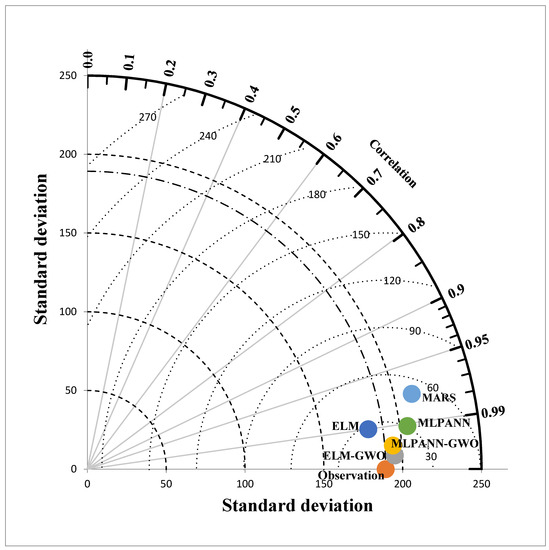
Figure 11.
Taylor diagram of the observed and predicted BOD5 concentrations for single- and two-stage ML models.
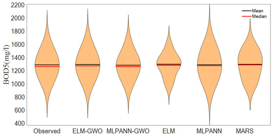
Figure 12.
Violin plot of the observed and predicted BOD5 concentrations for single- and two-stage ML models.
4.2. Predicting the Turbidity and EC Indicators in the Groundwater Quality of the Saravan Landfill
4.2.1. Application of Single- and Two-Stage ML Models for the Turbidity Indicator
The predictive evaluation of different ML models conditional on four statistical measures for the turbidity indicator is presented in Table 3. It shows that the predictive evaluation of the ELM-GWO (RMSE = 0.061 NTU, NS = 0.989, and MAE = 0.045 NTU) model was better compared to that of the MARS, MLPANN, ELM, and MLPANN-GWO models in the groundwater quality of the Saravan landfill during the testing phase.
Table 3.
Testing results of the applied models for predicting the turbidity value in groundwater quality assessment.
Figure 13a–e show the scatter plots of the observed and predicted turbidity indicator values for single- and two-stage ML models. The fitted line, matching line, and statistical measure (R) value are present in the equivalent scatter plots. It can be observed from Figure 13a–e that an obvious difference can be seen between the single- and two-stage ML models. In other words, the ELM-GWO model had a superior statistical measure (R = 0.997) between the single- and two-stage ML models.
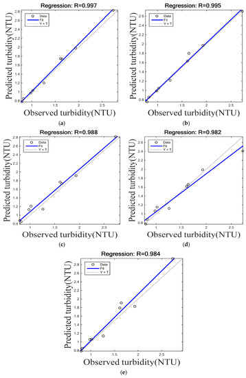
Figure 13.
Scatter plots of the observed and predicted turbidity values for the single- and two-stage ML models: (a) ELM-GWO, (b) MLPANN-GWO, (c) ELM, (d) MLPANN, and (e) MARS.
To confirm the reliable predictive performance employing visual assistance, the Taylor diagram (Figure 14) shows the best performance of the ELM-GWO model compared to other single- and two-stage ML models for the turbidity indicator because the ELM-GWO model has the nearest distance for the observed values of the turbidity indicator compared to other single- and two-stage ML models. Additionally, the violin plot (Figure 15) shows similar results for the ELM-GWO, MLPANN-GWO, and MLPANN models regarding the observed values of the turbidity indicator based on single- and two-stage ML models in the groundwater quality of the Saravan landfill.
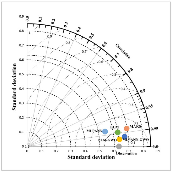
Figure 14.
Taylor diagram of the observed and predicted turbidity values for single- and two-stage ML models.
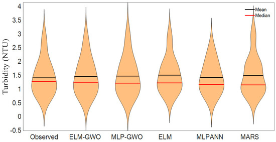
Figure 15.
Violin plot of the observed and predicted turbidity values for single- and two-stage ML models.
4.2.2. Application of Single- and Two-Stage ML Models for the EC Indicator
The predictive judgement of the diverse ML models conditional on four statistical measures for the EC indicator is shown in Table 4. Additionally, it shows that the predictive evaluation of the ELM-GWO (RMSE = 7.66 S/cmµ, NS = 0.990, and MAE = 6.65 S/cmµ) model was better compared to that of the MARS, MLPANN, ELM, and MLPANN-GWO models in the groundwater quality of the Saravan landfill during the testing phase.
Table 4.
Testing results of the applied models for predicting the EC value in groundwater quality assessment.
Figure 16a–e present the scatter plots of the observed and predicted EC indicator values for single- and two-stage ML models. The blue solid (fitted) line, dotted (matching) line, and statistical measure (R) value are shown in each scatter plots. It can be observed from Figure 16a–e that a distinct divergence can be noticed between the single- and two-stage ML models. Especially, the ELM-GWO model had the best statistical measure (R = 0.997) between the single- and two-stage ML models.
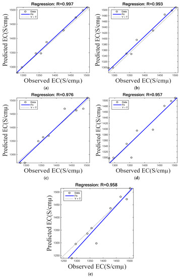
Figure 16.
Scatter plots of the observed and predicted EC values for single- and two-stage ML models: (a) ELM-GWO, (b) MLPANN-GWO, (c) ELM, (d) MLPANN, and (e) MARS.
To approve the predictive efficiency utilizing visual assessment, the Taylor diagram (Figure 17) shows the superior efficiency of the ELM-GWO model compared to other single- and two-stage ML models for the EC indicator since the ELM-GWO model had the shortest distance to reach the observed value of the turbidity indicator. Likewise, the violin plot (Figure 18) supplies similar shapes for the ELM-GWO, MLPANN-GWO, and MLPANN models regarding the observed values of the EC indicator dependent on single- and two-stage ML models in the groundwater quality of the Saravan landfill.
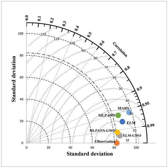
Figure 17.
Taylor diagram of the observed and predicted EC values for single- and two-stage ML models.
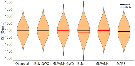
Figure 18.
Violin plot of the observed and predicted EC values for single- and two-stage ML models.
Figure 19a–d show a comparison of the RMSE values of single- and two-stage ML models for predicting the explained water quality parameters (i.e., COD, BOD5, turbidity, and EC). It can be found from Figure 19a–d that the ELM-GWO model provided the lowest RMSE values, whereas the MARS model was the opposite. That is, the ELM-GWO model was the best model for predicting the leachate and groundwater quality in the landfill site. In addition, Figure 20a–d presents a comparison of the MAE values of single- and two-stage ML models for predicting the explained water quality parameters. It can be observed from Figure 20a–d that the ELM-GWO model is the best model compared to other single- and two-stage ML models for the prediction of leachate and groundwater quality in the landfill site, while the MARS model is the opposite. In other words, ELM-GWO is the best model for the prediction of leachate and groundwater quality in the landfill site.
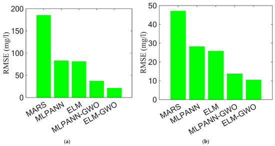
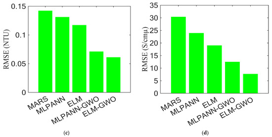
Figure 19.
Comparison of the RMSE values of single- and two-stage ML models for the prediction of (a) COD, (b) BOD5, (c) turbidity, and (d) EC.
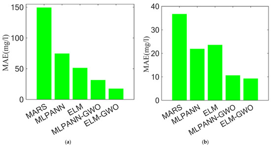
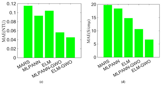
Figure 20.
Comparison of the MAE values of single- and two-stage ML models for the prediction of (a) COD, (b) BOD5, (c) turbidity, and (d) EC.
5. Discussion
The current research conducted the predictive achievement of four water quality parameters (i.e., COD, BOD5, turbidity, and EC) by applying single- and two-stage machine learning models in the leachate and groundwater quality of the Saravan landfill, Iran. The current research procedure followed two procedures. First, COD and BOD5 concentration were investigated utilizing single- and two-stage ML models in the leachate quality of the landfill site. Second, as the next procedure, turbidity and EC indicators were assessed based on single- and two-stage ML models. ELM-GWO, one of two-stage ML models, had the best predictive performance in the four water quality parameters in the groundwater quality of the landfill site during the testing phase.
The essential purpose for employing two-stage ML models is to build a predictive performance assessment of four water quality parameters (COD, BOD5, turbidity, and EC) of single-stage ML models. In the current research, the MARS model was not combined into a two-stage ML model (e.g., MARS-GWO). As the results of the models’ application, all the two-stage ML models (ELM-GWO and MLPANN-GWO) could increase the predictive reliability of the corresponding single-stage ML models (ELM and MLPANN) for COD, BOD5, turbidity, and EC relying on the values of four statistical measures (RMSE, NS, R, and MAE) in the leachate and groundwater quality of the landfill site.
Considering the MLPANN-GWO model conditional on the MAE statistical measure, COD (137.09% by MLPANN), BOD5 (106.72% by MLPANN), turbidity (66.07% by MLPANN), and EC (73.23% by MLPANN) improved the predictive efficiency of the above water quality parameters. In the case of the ELM-GWO model, COD (193.57 % by ELM), BOD5 (155.59% by ELM), turbidity (131.11% by ELM), and EC (121.81% by ELM) boosted the predictive reliability of the explained water quality parameters.
Acknowledging the accomplishment of two-stage ML models (MLPANN-GWO and ELM-GWO) dependent on the values of MAE statistical measure in the leachate and groundwater quality of the landfill site, the COD concentration provided the best results based on the corresponding single-stage ML models (MLPANN and ELM) compared to the other parameters (BOD5, turbidity, and EC). In addition, the water quality parameters of the leachate quality provided the better improvement than those of the groundwater quality in the landfill site.
Additionally, recognizing the previous articles and reports for the prediction of water quality parameters conditional on ML and deep learning (DL) models in the leachate and groundwater quality of the landfill site, Azadi et al. (2016) developed ANN and principal component analysis-M5P (PCA-M5P) to predict the COD concentration in leachates provided by the lab-scale landfills, in Bangladesh. They demonstrated that ANN performed better accuracy for predicting COD concentration compared to PCA-M5P [1]. Ishii et al. (2022) employed long short-term memory (LSTM) for predicting leachate quality, including COD, BOD, Cl, Ca, and total nitrogen (T-N) parameters, in a landfill area in Japan [2]. The research of Ishii et al. (2022) demonstrated the predictive processes of leachate quality and quantity and supplied the possibility of LSTM for future operation and management of landfill areas. In addition, similar research, which employed ML and DL models for predicting groundwater quality parameters, can be found in the previous documents.
Band et al. (2020) applied four single-stage ML models (i.e., Bayesian artificial neural network (BANN), Cubist, random forest (RF), and support vector machine (SVM)) to estimate the groundwater nitrate concentration in Iran. They concluded that the north part of the research area provided the highest groundwater nitrate concentration compared to other parts of research area [51]. Singha et al. (2021) predicted groundwater quality parameters utilizing four single-stage ML and DL models (i.e., DL, ANN, RF, and extreme gradient boosting (EGB)) in India. The results showed that DL model had the best accuracy compared to the other developed models [52]. In addition, Abba et al. (2023) applied two-stage ML models combining adaptive neuro-fuzzy inference system (ANFIS) and three metaheuristic optimization algorithms (i.e., genetic algorithm (GA), biogeography-based optimization (BBO), and PSO) to predict the groundwater salinization of coastal region in Saudi Arabia. They showed that ANFIS-PSO had the best accuracy for predicting groundwater salinization compared to ANFIS-GA and ANFIS-BBO [53]. Moayedi et al. (2023) predicted groundwater quality parameters employing two-stage ML models combining ANN and three metaheuristic optimization algorithms (i.e., artificial bee colony (ABC), Harris hawks optimization (HHO), and GWO), Iran. This research illustrated that ANN-GWO provided the best prediction compared to ANN-HHO and ANN-ABC [28].
In the current research, since the prediction of leachate and groundwater quality in the landfill site focused on a few machine learning models and evolutionary optimization algorithms, our method for predicting leachate and groundwater quality cannot strengthen the reliability and credibility of the employed tools. The diverse application of the employed tools is required to boost the predictive efficiency of leachate and groundwater quality in landfill sites.
6. Conclusions
One of the important sources of the pollution of surface water and groundwater is landfill leachate. This research focused on the prediction of leachate quality by considering COD and BOD5 as target parameters and also groundwater quality by employing turbidity and EC as response parameters. The observed dataset was gathered from the Saravan landfill, Rast, Iran. Then, two different types of artificial intelligence models, including single-stage (MARS, MLPANN, and ELM) and two-stage (MLPANN-GWO and ELM-GWO) paradigms, were applied for predicting COD and BOD5 parameters for analyzing landfill leachate quality; turbidity and EC parameters were also employed for assessing groundwater quality. The results obtained from both leachate quality and groundwater quality parameters indicate that ELM-GWO significantly improved the performance in terms of the RMSE measure of the MLPANN-GWO, ELM, MLPANN, and MARS models by 43.07%, 73.88%, 74.5%, and 88.55% for the COD parameter; 23.91%, 59.31%, 62.85%, and 77.71% for the BOD5 parameter; 14.08%, 47.86%, 53.43%, and 57.04% for turbidity; and 38.57%, 59.64%, 67.94%, and 74.76% for the EC value, respectively. This study suggests that ELM-GWO can be a robust alternative to MARS, MLPANN, ELM, and MLPANN-GWO in leachate quality and groundwater quality applications and the proposed framework can be utilized by landfill authorities and decision makers for implementing reliable strategies.
Author Contributions
Conceptualization and data analysis, M.A.; Project administration and Supervision, M.A.; Software, M.A.; Methodology, S.H.; Writing—Original draft preparation, Writing—Review & Editing, S.K.; Writing—Original draft preparation, Writing—Review & Editing, O.K.; Writing—Original draft preparation, Writing—Review & Editing, M.K.; Writing—Review & Editing, Z.K. (Zahra Kazemi); Writing—Review & Editing, Z.K. (Zohre Kazemi); Writing—Review & Editing, I.-M.C. All authors have read and agreed to the published version of the manuscript.
Funding
This research received no external funding.
Acknowledgments
This work was supported financially by the Iran University of Medical Sciences, Tehran, Iran (No. 1401-4-2-24594). Also, this research was supported by a grant from the Development Program of Minimizing of Climate Change Impact Technology funded through the National Research Foundation of Korea (NRF) of the Korean government (Ministry of Science and ICT, Grant No. NRF-2020M3H5A1080735).
Conflicts of Interest
The authors declare no conflict of interest.
References
- Azadi, S.; Amiri, H.; Rakhshandehroo, G.R. Evaluating the ability of artificial neural network and PCA-M5P models in predicting leachate COD load in landfills. Waste Manag. 2016, 55, 220–230. [Google Scholar] [CrossRef] [PubMed]
- Ishii, K.; Sato, M.; Ochiai, S. Prediction of leachate quantity and quality from a landfill site by the long short-term memory model. J. Environ. Manag. 2022, 310, 114733. [Google Scholar] [CrossRef] [PubMed]
- Schroeder, P.R.; Peyton, R.L. Verification of the Hydrologic Evaluation of Landfill Performance (HELP) Model Using Field Data; Hazardous Waste Engineering Research Laboratory, Office of Research and Development, US Environmental Protection Agency: Cincinnati, OH, USA, 1988. [Google Scholar]
- Jalilzadeh, H.; Hettiaratchi, J.P.A.; Fleming, I.; Pokhrel, D. Effect of soil type and vegetation on the performance of evapotranspirative landfill biocovers: Field investigations and water balance modeling. J. Hazard. Toxic Radioact. Waste 2020, 24, 04020046. [Google Scholar] [CrossRef]
- Ghiasinejad, H.; Ghasemi, M.; Pazoki, M.; Shariatmadari, N. Prediction of landfill leachate quantity in arid and semiarid climate: A case study of Aradkouh, Tehran. Int. J. Environ. Sci. Technol. 2021, 18, 589–600. [Google Scholar] [CrossRef]
- Riester, J.E., Jr. Landfilled Leachate Production and Gas Generation Numerical Model. Ph.D. Thesis, Old Dominion University, Norfolk, VA, USA, 1994. [Google Scholar]
- Fellner, J.; Brunner, P.H. Modeling of leachate generation from MSW landfills by a 2-dimensional 2-domain approach. Waste Manag. 2010, 30, 2084–2095. [Google Scholar] [CrossRef]
- Illiano, D.; Pop, I.S.; Radu, F.A. Iterative schemes for surfactant transport in porous media. Comput. Geosci. 2021, 25, 805–822. [Google Scholar] [CrossRef]
- Hubert, J.; Liu, X.F.; Collin, F. Numerical modeling of the long term behavior of Municipal Solid Waste in a bioreactor landfill. Comput. Geotech. 2016, 72, 152–170. [Google Scholar] [CrossRef]
- Reddy, K.R.; Kumar, G.; Giri, R.K. Influence of dynamic coupled hydro-bio-mechanical processes on response of municipal solid waste and liner system in bioreactor landfills. Waste Manag. 2017, 63, 143–160. [Google Scholar] [CrossRef]
- Shu, S.; Zhu, W.; Shi, J. A new simplified method to calculate breakthrough time of municipal solid waste landfill liners. J. Clean. Prod. 2019, 219, 649–654. [Google Scholar] [CrossRef]
- Lee, Y.S.; Kim, Y.M.; Lee, J.; Kim, J.Y. Evaluation of silver nanoparticles (AgNPs) penetration through a clay liner in landfills. J. Hazard. Mater. 2021, 404, 124098. [Google Scholar] [CrossRef]
- Yu, F.; Wu, Z.; Wang, J.; Li, Y.; Chu, R.; Pei, Y.; Ma, J. Effect of landfill age on the physical and chemical characteristics of waste plastics/microplastics in a waste landfill sites. Environ. Pollut. 2022, 306, 119366. [Google Scholar] [CrossRef] [PubMed]
- Nordin, N.F.; Mohd, N.S.; Koting, S.; Ismail, Z.; Sherif, M.; El-Shafie, A. Groundwater quality forecasting modelling using artificial intelligence: A review. Groundw. Sustain. Dev. 2021, 14, 100643. [Google Scholar] [CrossRef]
- Azadi, S.; Karimi-Jashni, A.; Javadpour, S. Modeling and optimization of photocatalytic treatment of landfill leachate using tungsten-doped TiO2 nano-photocatalysts: Application of artificial neural network and genetic algorithm. Process Saf. Environ. Prot. 2018, 117, 267–277. [Google Scholar] [CrossRef]
- Roudi, A.M.; Chelliapan, S.; Mohtar, W.H.M.W.; Kamyab, H. Prediction and optimization of the Fenton process for the treatment of landfill leachate using an artificial neural network. Water 2018, 10, 595. [Google Scholar] [CrossRef]
- Masouleh, S.Y.; Mozaffarian, M.; Dabir, B.; Ramezani, S.F. COD and ammonia removal from landfill leachate by UV/PMS/Fe2+ process: ANN/RSM modeling and optimization. Process Saf. Environ. Prot. 2022, 159, 716–726. [Google Scholar] [CrossRef]
- Bhatt, A.H.; Altouqi, S.; Karanjekar, R.V.; Sahadat Hossain, M.D.; Chen, V.P.; Sattler, M.S. Preliminary regression models for estimating first-order rate constants for removal of BOD and COD from landfill leachate. Environ. Technol. Innov. 2016, 5, 188–198. [Google Scholar] [CrossRef]
- Bhatt, A.H.; Karanjekar, R.V.; Altouqi, S.; Sattler, M.L.; Hossain, M.D.S.; Chen, V.P. Estimating landfill leachate BOD and COD based on rainfall, ambient temperature, and waste composition: Exploration of a MARS statistical approach. Environ. Technol. Innov. 2017, 8, 1–16. [Google Scholar] [CrossRef]
- Ahmad, W.; Ayub, N.; Ali, T.; Irfan, M.; Awais, M.; Shiraz, M.; Glowacz, A. Towards short term electricity load forecasting using improved support vector machine and extreme learning machine. Energies 2020, 13, 2907. [Google Scholar] [CrossRef]
- Chen, Y.; Zhang, X.; Karimian, H.; Xiao, G.; Huang, J. A novel framework for prediction of dam deformation based on extreme learning machine and Lévy flight bat algorithm. J. Hydroinformatics 2021, 23, 935–949. [Google Scholar] [CrossRef]
- Deka, P.C.; Patil, A.P.; Kumar, P.Y.; Naganna, S.R. Estimation of dew point temperature using SVM and ELM for humid and semi-arid regions of India. ISH J. Hydraul. Eng. 2018, 24, 190–197. [Google Scholar] [CrossRef]
- Liu, C.; Fu, Q.; Li, T.; Imran, K.M.; Cui, S.; Abrar, F.M.; Liu, D. ELM evaluation model of regional groundwater quality based on the crow search algorithm. Ecol. Indic. 2017, 81, 302–314. [Google Scholar] [CrossRef]
- Mirjalili, S.; Mirjalili, S.M.; Lewis, A. Grey Wolf Optimizer. Adv. Eng. Softw. 2014, 69, 46–61. [Google Scholar] [CrossRef]
- Shahin, I.; Alomari, O.A.; Nassif, A.B.; Afyouni, I.; Hashem, I.A.; Elnagar, A. An efficient feature selection method for arabic and english speech emotion recognition using Grey Wolf Optimizer. Appl. Acoust. 2023, 205, 109279. [Google Scholar] [CrossRef]
- Ghobadi, A.; Cheraghi, M.; Sobhanardakani, S.; Lorestani, B.; Merrikhpour, H. Groundwater quality modeling using a novel hybrid data-intelligence model based on gray wolf optimization algorithm and multi-layer perceptron artificial neural network: A case study in Asadabad Plain, Hamedan, Iran. Environ. Sci. Pollut. Res. 2022, 29, 8716–8730. [Google Scholar] [CrossRef] [PubMed]
- Fadhillah, M.F.; Lee, S.; Lee, C.W.; Park, Y.C. Application of support vector regression and metaheuristic optimization algorithms for groundwater potential mapping in gangneung-si, South Korea. Remote Sens. 2021, 13, 1196. [Google Scholar] [CrossRef]
- Moayedi, H.; Salari, M.; Dehrashid, A.A.; Le, B.N. Groundwater quality evaluation using hybrid model of the multi-layer perceptron combined with neural-evolutionary regression techniques: Case study of Shiraz plain. Stoch. Environ. Res. Risk Assess. 2023. [Google Scholar] [CrossRef]
- Lee, A.H.; Nikraz, H. BOD:COD Ratio as an Indicator for Pollutants Leaching from Landfill. J. Clean Energy Technol. 2014, 2, 263–266. [Google Scholar] [CrossRef]
- Friedman, J.H. Multivariate adaptive regression splines. Ann. Stat. 1991, 19, 1–67. [Google Scholar] [CrossRef]
- Abdi, J.; Pirhoushyaran, T.; Hadavimoghaddam, F.; Madani, S.A.; Hemmati-Sarapardeh, A.; Esmaeili-Faraj, S.H. Modeling of capacitance for carbon-based supercapacitors using Super Learner algorithm. J. Energy Storage 2023, 66, 107376. [Google Scholar] [CrossRef]
- Shiau, J.; Keawsawasvong, S. Multivariate adaptive regression splines analysis for 3D slope stability in anisotropic and heterogenous clay. J. Rock Mech. Geotech. Eng. 2023, 15, 1052–1064. [Google Scholar] [CrossRef]
- Alizamir, M.; Shiri, J.; Fard, A.F.; Kim, S.; Gorgij, A.D.; Heddam, S.; Singh, V.P. Improving the accuracy of daily solar radiation prediction by climatic data using an efficient hybrid deep learning model: Long short-term memory (LSTM) network coupled with wavelet transform. Eng. Appl. Artif. Intell. 2023, 123, 106199. [Google Scholar] [CrossRef]
- Ashrafian, A.; Panahi, E.; Salehi, S.; Karoglou, M.; Asteris, P.G. Mapping the strength of agro-ecological lightweight concrete containing oil palm by-product using artificial intelligence techniques. Structures 2023, 48, 1209–1229. [Google Scholar] [CrossRef]
- Saha, S.; Bera, B.; Shit, P.K.; Bhattacharjee, S.; Sengupta, N. Prediction of forest fire susceptibility applying machine and deep learning algorithms for conservation priorities of forest resources. Remote Sens. Appl. Soc. Environ. 2023, 29, 100917. [Google Scholar] [CrossRef]
- Huang, G.B.; Chen, L.; Siew, C.K. Universal approximation using incremental constructive feedforward networks with random hidden nodes. IEEE Trans. Neural Netw. 2006, 17, 879–892. [Google Scholar] [CrossRef] [PubMed]
- Huang, G.B.; Zhu, Q.Y.; Siew, C.K. Extreme learning machine: Theory and applications. Neurocomputing 2006, 70, 489–501. [Google Scholar] [CrossRef]
- Alizamir, M.; Kim, S.; Kisi, O.; Zounemat-Kermani, M. Deep echo state network: A novel machine learning approach to model dew point temperature using meteorological variables. Hydrol. Sci. J. 2020, 65, 1173–1190. [Google Scholar] [CrossRef]
- Alizamir, M.; Heddam, S.; Kim, S.; Mehr, A.D. On the implementation of a novel data-intelligence model based on extreme learning machine optimized by bat algorithm for estimating daily chlorophyll-a concentration: Case studies of river and lake in USA. J. Clean. Prod. 2021, 285, 124868. [Google Scholar] [CrossRef]
- Yuan, Z.; Xiong, G.; Fu, X.; Mohamed, A.W. Improving fault tolerance in diagnosing power system failures with optimal hierarchical extreme learning machine. Reliab. Eng. Syst. Saf. 2023, 236, 109300. [Google Scholar] [CrossRef]
- Kisi, O.; Alizamir, M.; Docheshmeh Gorgij, A. Dissolved oxygen prediction using a new ensemble method. Environ. Sci. Pollut. Res. 2020, 27, 9589–9603. [Google Scholar] [CrossRef]
- Xu, Q.; Wei, X.; Bai, R.; Li, S.; Meng, Z. Integration of deep adaptation transfer learning and online sequential extreme learning machine for cross-person and cross-position activity recognition. Expert Syst. Appl. 2023, 212, 118807. [Google Scholar] [CrossRef]
- Alizamir, M.; Kisi, O.; Kim, S.; Heddam, S. A novel method for lake level prediction: Deep echo state network. Arab. J. Geosci. 2020, 13, 956. [Google Scholar] [CrossRef]
- Alizamir, M.; Heddam, S.; Kim, S.; Gorgij, A.D.; Li, P.; Ahmed, K.O.; Singh, V.P. Prediction of daily chlorophyll-a concentration in rivers by water quality parameters using an efficient data-driven model: Online sequential extreme learning machine. Acta Geophys. 2021, 69, 2339–2361. [Google Scholar] [CrossRef]
- Kisi, O.; Alizamir, M. Modelling reference evapotranspiration using a new wavelet conjunction heuristic method: Wavelet extreme learning machine vs wavelet neural networks. Agric. For. Meteorol. 2018, 263, 41–48. [Google Scholar] [CrossRef]
- Alizamir, M.; Kim, S.; Zounemat-Kermani, M.; Heddam, S.; Shahrabadi, A.H.; Gharabaghi, B. Modelling daily soil temperature by hydro-meteorological data at different depths using a novel data-intelligence model: Deep echo state network model. Artif. Intell. Rev. 2021, 54, 2863–2890. [Google Scholar] [CrossRef]
- Haykin, S. Neural Networks a Comprehensive Foundation; Prentice Hall: Upper Saddle River, NJ, USA, 1999. [Google Scholar]
- Hornik, K. Approximation capabilities of multilayer feedforward networks. Neural Netw. 1991, 4, 251–257. [Google Scholar] [CrossRef]
- Taylor, K.E. Summarizing multiple aspects of model performance in a single diagram. J. Geophys. Res. Atmos. 2001, 106, 7183–7192. [Google Scholar] [CrossRef]
- Hintze, J.L.; Nelson, R.D. Violin plots: A box plot-density trace synergism. Am. Stat. 1998, 52, 181–184. [Google Scholar]
- Band, S.S.; Janizadeh, S.; Pal, S.C.; Chowdhuri, I.; Siabi, Z.; Norouzi, A.; Melesse, A.M.; Shokri, M.; Mosavi, A. Comparative analysis of artificial intelligence models for accurate estimation of groundwater nitrate concentration. Sensors 2020, 20, 5763. [Google Scholar] [CrossRef]
- Singha, S.; Pasupuleti, S.; Singha, S.S.; Singh, R.; Kumar, S. Prediction of groundwater quality using efficient machine learning technique. Chemosphere 2021, 276, 130265. [Google Scholar] [CrossRef]
- Abba, S.I.; Benaafi, M.; Usman, A.G.; Ozsahin, D.U.; Tawabini, B.; Aljundi, I.H. Mapping of groundwater salinization and modelling using meta-heuristic algorithms for the coastal aquifer of eastern Saudi Arabia. Sci. Total Environ. 2023, 858, 159697. [Google Scholar] [CrossRef]
Disclaimer/Publisher’s Note: The statements, opinions and data contained in all publications are solely those of the individual author(s) and contributor(s) and not of MDPI and/or the editor(s). MDPI and/or the editor(s) disclaim responsibility for any injury to people or property resulting from any ideas, methods, instructions or products referred to in the content. |
© 2023 by the authors. Licensee MDPI, Basel, Switzerland. This article is an open access article distributed under the terms and conditions of the Creative Commons Attribution (CC BY) license (https://creativecommons.org/licenses/by/4.0/).