Multistep Flood Inundation Forecasts with Resilient Backpropagation Neural Networks: Kulmbach Case Study

Abstract

Flooding, a significant natural disaster, attracts worldwide attention because of its high impact on communities and individuals and increasing trend due to climate change. A flood forecast system can minimize the impacts by predicting the flood hazard before it occurs. Artificial neural networks (ANN) could efficiently process large amounts of data and find relations that enable faster flood predictions. The aim of this study is to perform multistep forecasts for 1–5 h after the flooding event has been triggered by a forecast threshold value. In this work, an ANN developed for the real-time forecast of flood inundation with a high spatial resolution (4 m × 4 m) is extended to allow for multiple forecasts. After trained with 120 synthetic flood events, the ANN was first tested with 60 synthetic events for verifying the forecast performance for 3 h, 6 h, 9 h and 12 h lead time. The model produces good results, as shown by more than 81% of all grids having an RMSE below 0.3 m. The ANN is then applied to the three historical flood events to test the multistep inundation forecast. For the historical flood events, the results show that the ANN outputs have a good forecast accuracy of the water depths for (at least) the 3 h forecast with over 70% accuracy (RMSE within 0.3 m), and a moderate accuracy for the subsequent forecasts with (at least) 60% accuracy.

1. Introduction

Floods are one of the most threatening hazards to civilian safety and infrastructures, causing damages and losses over the world [1]. Especially in densely populated urban areas, urbanization, aging of drainage systems and climate change contribute to growing flood risk in many countries. Ione important mitigation measure is the prediction of future flood occurrences. Real-time flood forecast with sufficient lead time can boost the use of preventive measures for flood mitigation. Such measures can minimize the threats to communities and individuals at risk of flooding [2].

Various types of hydrology and hydraulic models are available for flood forecasting [3]. From the different modeling types, these can be classified into rainfall-runoff models, one-dimensional (1D) model, two-dimensional (2D) model, and coupled 1D–1D model and 1D–2D model. From the forecast application perspective, 2D and 1D–2D models are able to provide directly a spatial surface flood representation, which is essential for flood damage estimation. 1D–1D models, on the other hand, relies heavily on GIS pre- and post-treatments. Most 2D hydrodynamic models are computationally expensive [4]. Even with the help of up-to-date computational techniques for 2D simulations, the computational capability is still inadequate for a real-time forecast [5].

Data-driven is a fast-growing alternative to hydrodynamic models due to the development of computing technologies in recent years. Data-driven models ignore the physical background of a problem and rather explore the relation between the input and output data [6]. For short or long-term flood forecasts, different data-driven models have been implemented, such as neuro-fuzzy [7], support vector machine [8], support vector regression [9,10], Bayesian linear regression methods [11] and artificial neural network (ANN) [12]. Among them, artificial neural networks (ANN) can be an effective tool for flood modeling, if it is properly applied, overcoming pitfalls as over-fitting/under-fitting with sufficient and representative data for model training [13]. Dawson and Wilby applied ANN to conventional hydrological models in flood-inclined catchments in the UK in 1998 [14]. After that, numerous examinations about flood forecasts in catchment scales emerged [2], [15]. Sit and Demir [16] integrated the river network spatial information to improve the forecast accuracy in Iowa. Bustami et al. applied the backpropagation ANN model for forecasting water levels at gauging stations [17]. ANN showed its great potential on the short-time forecast of extreme water levels with a comparable accuracy to the physical model with a far less computational cost [18]. Simon Berkhahn et al. applied an ANN for two-dimensional (2D) urban pluvial inundation extent forecast [19]. Lin et al. applied backpropagation networks for maximum flood inundation extent prediction and achieved a comparable accuracy to the hydraulic model [20].

The objective of this work is to develop a multistep flood forecast method for urban areas at a fine spatial resolution of 4 m by 4 m. Unlike Lin et al. [20], in this study, an ANN-based framework is proposed for performing multistep forecasts for 1–5 h. To the author’s knowledge, only the works of Chang et al. [2] and Shen and Chang [21] were able to produce multistep flood forecasting maps. The novelty herein is the forecast at a finer resolution of 4 m × 4 m, suitable for urban flood forecast. Our hypothesis is that the ANN forecast model can provide comparably accurate flood extents as hydraulic models, but with a much shorter time of several seconds. As the hydrodynamics-based model runs usually takes several hours, the reduction in forecast time of ANN enables more flood mitigation measures to become effective. In Section 2, we introduce the resilient backpropagation artificial neural network structure and the validation of the model. Section 3 describes the study area and the data preparation of the event database. Section 4 shows the results of flood forecasts of the first intervals for synthetic and historical flood events and the real-time forecast for historical flood events. Section 5 and Section 6 are the discussion and conclusion of this work.

2. Methods

2.1. Data and Structure of Artificial Neural Networks

Artificial neural networks are algorithms applied to map features into a series of outputs. Through a structure of the input, output and intermediate hidden layers, artificial neural networks can learn data relationships between input and output data [22]. A feedforward neural network is applied in this work for modeling the study area, proceeding and transmitting data in a network structure [23]. One of the most widely used ANN is the multilayer perceptron (MLP) [24]. The MLP consists of highly interconnected neurons organized in layers to process information. The neurons in one layer are fully connected to each neuron in the next layer. Each connection is then assigned a weight. Each neuron collects values from the previous layer by summing up the results from the previous neuron values multiplying the weight on each input arcs and storing the results on itself. An activation function is used to transfer the results from the hidden layers to the output layer, and a loss function is applied to measure the fit of the neural network to a set of input–output data pair.

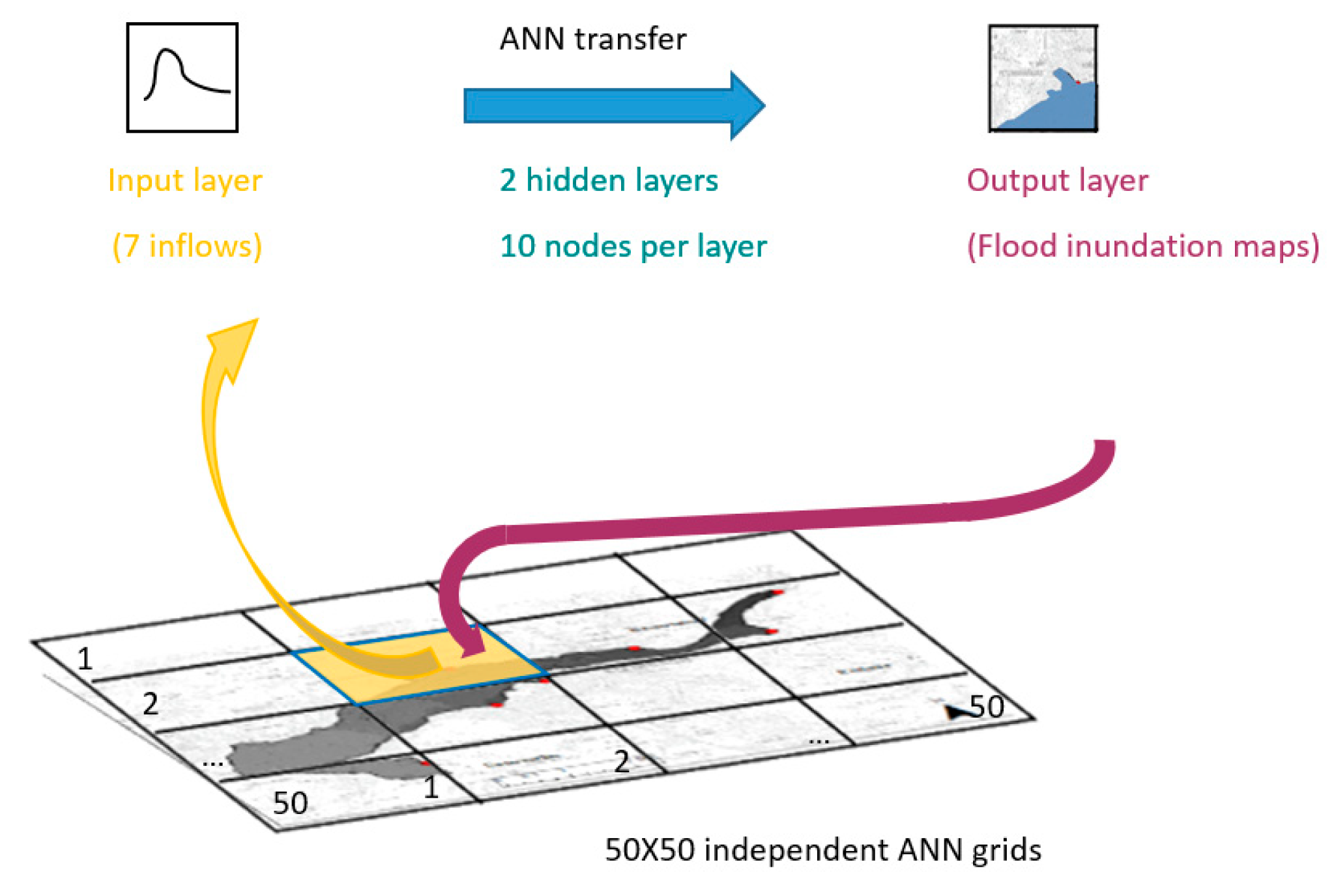
In this case study, the input layer collects the seven inflows to the urban area of Kulmbach, given the hourly discharge intensity. The output layer is fed with the hourly raster inundation map with a resolution of 4 m × 4 m from the event database. Between the input layer and the output layer, the ANN has 2 hidden layers with 10 nodes per layer. One hundred twenty synthetic events from the event database are used for network training (see Section 3.2). Afterward, the other 60 events in the event database are used for model validation. This represents 2/3 of the date for training and 1/3 for testing, which is often found in the literature [25]. Finally, the model is applied to forecast three historical events. The widely applied sigmoid function is chosen as the activation function for the neural network [26]. Due to the high-resolution of the map (4 m by 4 m), weights between the last hidden layer and the output layer would have been 1 GB RAM with a dimension of the problem of more than 30 million. The optimization of these weights is very time-consuming, even with the latest optimization techniques [27]. Hence, a “divide and conquer” strategy is used to enable calculation in a single PC. In addition, it should be noted that, in principle, the results of the two strategies should be the same. Some alternative artificial network structures, such as a convolutional neural network (CNN), could not be applied in this study. The network size would require a very large number of hypermeters, which was beyond the memory capacity of a personal computer for forecasting purposes [28]. Furthermore, the time for training can be reduced with our strategy due to parallelization. The estimated time for training all networks in parallel with four cores is 6 h. To reduce the training time and save memory requirements, the study area is divided into 50 × 50 squared grids (see Figure 1). A similar idea of splitting has been applied to a former study [19]. Each grid had four independent ANNs for intervals (3 h, 6 h, 9 h and 12 h). In total, 10,000 ANNs are trained to produce multistep forecasts.

2.2. Hyperparameter Tuning in ANN

To optimize weights in ANN, resilient backpropagation is a widely applied effective algorithm [29]. According to Shamim et al. and Panda et al. [23,30], backpropagation neural networks outperform other methods in flood forecasting studies for their more efficiency and higher robustness. Berkhahn et al. [19] compared the training algorithms for hyperparameter tuning. The authors showed that resilient backpropagation is more efficient than both backpropagation and Levenberg–Marquardt for maximum flood inundation prediction. The process has two stages: the training stage gathers information from the flood event database, changing the weights between layers to minimize the error on the output layer; the recalling stage generates the forecast for the rest of the events in the database for testing the model.

Formula 1 and Formula 2 show the scheme of a resilient backpropagation. To calculate the update of the network weights $w_{ij}$ from ith neuron to jth neuron, the gradient descent algorithm is applied. It distinguishes the update of weights upon the derivative of the loss function $L$ of the model. The loss function L takes the mean square error (MSE). The iteration stops once the loss function reaches its minimum (chosen 10⁻⁶ in this case).

$${\Delta }_{ij}\left(t\right)=\{\begin{array}{c}{\eta }^{+}·{\Delta }_{ij}\left(t-1\right), \frac{\partial L}{\partial w_{ij}}\left(t\right)·\frac{\partial L}{\partial w_{ij}}\left(t-1\right)>0\\ {\eta }^{-}·{\Delta }_{ij}\left(t-1\right), \frac{\partial L}{\partial w_{ij}}\left(t\right)·\frac{\partial L}{\partial w_{ij}}\left(t-1\right)<0\\ {\Delta }_{ij}\left(t-1\right), \mathrm{else}\end{array},$$

(1)

$$w_{ij}\left(t\right)=\{\begin{array}{c}{w}_{ij}\left(t-1\right)+{\Delta }_{ij}\left(t\right), \frac{\partial L}{\partial w_{ij}}\left(t\right)<0\\ w_{ij}\left(t-1\right)-{\Delta }_{ij}\left(t\right), \frac{\partial L}{\partial w_{ij}}\left(t\right)>0\\ 0, \mathrm{else}\end{array},$$

(2)

The learning rate is to scale the speed in each weight updating iteration. The larger alternative learning rate ${\eta }^{+}$ is chosen when the error gradient in the same signal in neighboring iterations and lower alternative learning rate ${\eta }^{-}$ when the loss function is close to zero, fulfilling $0<{\eta }^{-}<1<{\eta }^{+}$. In our study, these were set constant and equal to ${\eta }^{-}=0.5,{\eta }^{+}=1.2$. The deep learning toolbox of MATLAB version R2017a is used to form the forecasts.

2.3. Prediction of the First Interval of Flood Events

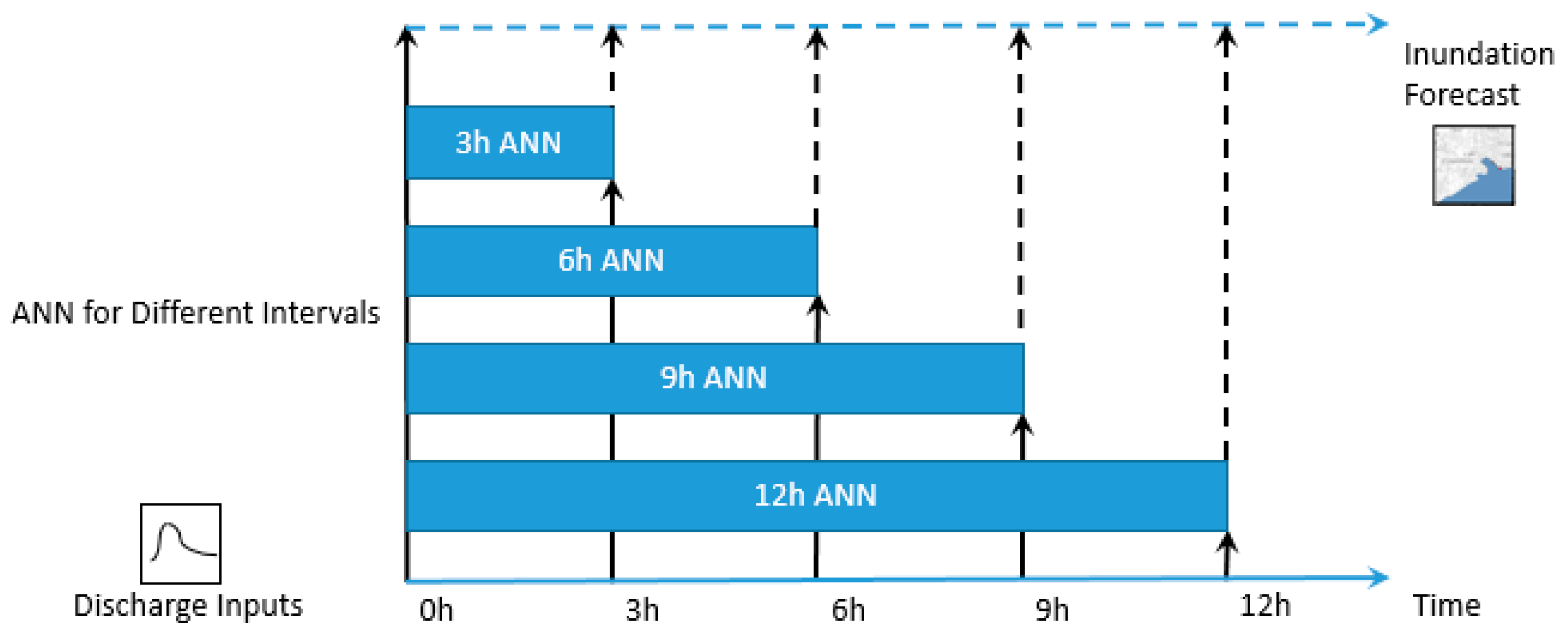
The ANN model is trained with the first 120 events in the synthetic flood event database (more details in Chapter 3.2). The time series of each event (starting from time 0) is extracted for training. The input inflow discharges are extracted from time 0 to X h (X takes the values from 3, 6, 9, 12). The respective output inundation maps at X h (X takes the values from 3, 6, 9, 12) are used as the output layer. The intervals of 3 h, 6 h, 9 h, 12 h of the flood events are used for training four networks with the same forecast lead times (see Figure 2). The ANN models only consider the input flow values from the initial time step (blue bars of the events in Figure 2), but not from the previous time steps. This was similar to the approach in the framework FloodEvac, which successfully produced forecasts based on the selection of pre-recorded flood maps [31].

After the training, the models are tested for the first interval forecast for the rest 60 events in the synthetic database.

2.4. Real-Time Forecasting for Sequential Multistep Forecast Intervals

In this work, the flood forecast starts when a certain discharge forecast threshold is achieved. If the start point occurs sometime later at time x, the prediction begin is also shifted to time x accordingly. If all the discharge inflows fall below the forecast threshold, the forecast is stopped. With this setup, the forecast can run in continuous mode.

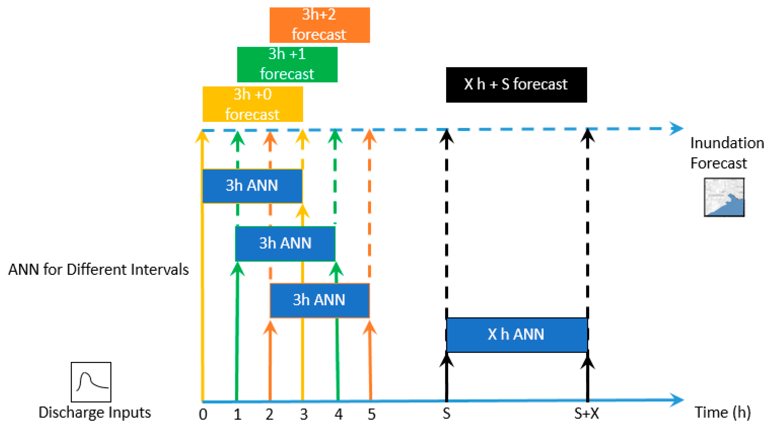
The ANN receives the corresponding discharge inputs of an interval, just as in real-time forecasts. After the forecast is complete for a certain step, the discharge forecast is repeated one hour ahead. The forecasts are done with the same ANN model, now starting one hour later, taking the discharge inputs from the next time interval. This procedure is repeated many times to enable the continuous mode of flood forecasting. In this case study, the real-time forecast is performed with the ANN models trained to forecast at multiple steps of 1–5 h. The forecast from time 0 and the shift forward of the forecast intervals by one hour and two hours are shown in Figure 3.

For an easier interpretation of the different forecast groups, we name each forecast as “X h + S” forecast. The “X h” indicates the forecast interval of X hours, and the “+ S” behind it shows the start time of the forecast.

2.5. Model Evaluation

The root-mean-square error (RMSE) is applied to access the ANN forecast performance in the study area. The forecasts of the ANN are compared against the inundation maps produced by the 2D dynamic model (see Section 3.2). Hence the 2D dynamic model results are assumed as the observed values in order to enable the evaluation of the ANN. Al, the events in the database have been processed by the FloodEvac tool [31] and validated [32]. As the ANN training is conducted within each grid, the RMSE is also evaluated for each grid.

$$\mathrm{RMSE}=\sqrt{\frac{1}{n}{\sum }_{i=1}^n{\left(T-S\right)}^2},$$

(3)

where

• T is the predicted value, water depth from the ANN model in our case.
• S is the observed value, water depth from the hydraulic model (HEC-RAS) in our case.
• To assess the general conduct of the model over the training and validation dataset, the average RMSE is also calculated for the average accuracy among all the events in the testing dataset.

To quantify the forecast of inundation extent growth, the following indices are used to measure the correspondence between the ANN model and the hydraulic model, namely probability of detection (POD), false alarm ratio (FAR) and critical success index (CSI) [33].

$$\mathrm{POD}=\frac{\mathrm{hits}}{\mathrm{hits}+\mathrm{misses}},$$

(4)

$$\mathrm{FAR}=\frac{\mathrm{false}\mathrm{alarms}}{\mathrm{hits}+\mathrm{false}\mathrm{alarms}},$$

(5)

$$\mathrm{CSI}=\frac{\mathrm{hits}}{\mathrm{hits}+\mathrm{misses}+\mathrm{false}\mathrm{alarms}},$$

(6)

A pixel with water depths under 10 cm is defined as a dry pixel, while over 10 cm as a wet pixel. Hits count the pixels that are both wet by the ANN forecast and the hydraulic simulation. Misses counting the pixels that are predicted dry by the ANN model but simulated wet by the hydraulic model. False alarms count the pixels predicted wet by ANN model but simulated dry by hydraulic model.

3. Study Area and Database

3.1. Study Area

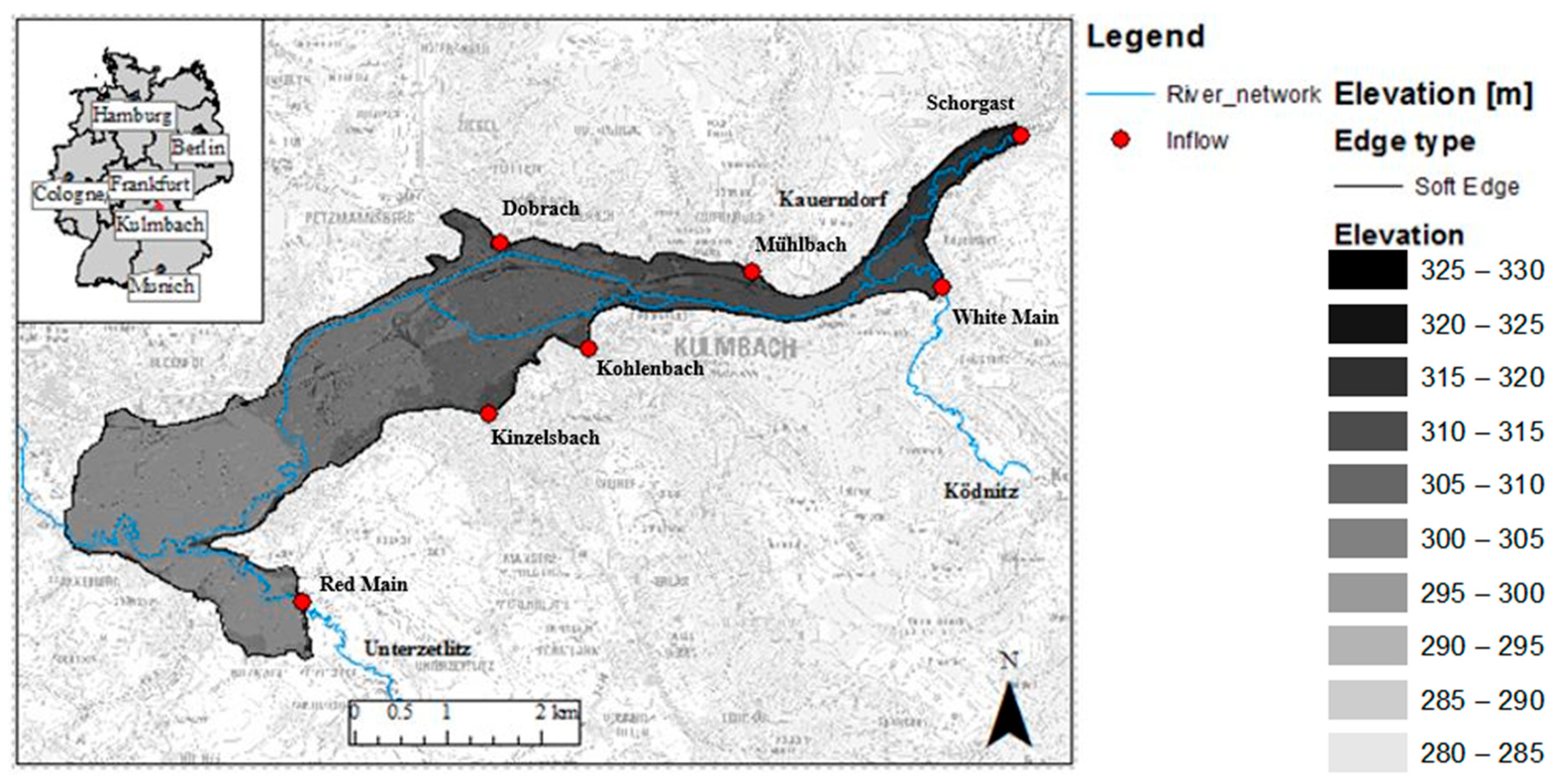
The study area of Kulmbach lies by the River Main in Bavaria, Germany. The White Main divides the city to the north and south parts. Seven streams, specifically the Red Main, White Main, Dobrach, Schorgast, Mühlbach, Kohlenbach and Kinzelsbach, flow into this area. The city Kulmbach has a population of 25, 866 inhabitants in an area of 92.77 km². An extreme flood event hit the city on 28 May 2006. A flood mitigation plan was prepared by local stakeholders to mitigate future events. In the ANN model, the above seven streams are taken as the input boundary conditions. The goal of the ANN modeling is to replace the hydraulic processes within the marked study area to enable fast real-time forecasts (see Figure 4).

3.2. HEC-RAS and Synthetic Event Database

The synthetic database is conducted by the 2D hydraulic model Hydrologic Engineering Center—river analysis system (HEC-RAS), Davis, CA, USA) for different precipitation durations, intensities and distributions [31]. Each event in the database contains a discharge hydrograph and an inundation map. The database contains 180 synthetic events in which discharge hydrographs are generated by the hydrologic model large area runoff simulation model (LARSIM) [34]. The events of the final database cover a wide range of different return periods, ranging from one year to 1.5 × 100 year return periods. The 2D hydrodynamic model HEC-RAS is used for producing the flood inundation maps. In the end, 180 hydrographs and their corresponding inundation maps form the synthetic event databases. The tool for automating these procedures is named the FloodEvac tool. The model is validated [32]. All the events are with a high temporal resolution of 15 min, and the inundation map is projected to a high spatial resolution (4 m by 4 m).

4. Results

The ANNs are trained for the first intervals (time 0). Thus, Section 4.1 focuses on assessing the results for the same time interval, which the ANNs are trained for. Section 4.2 focuses on the subsequent multistep forecast intervals. The aim is to verify if the hypothesis that the same ANNs can be used to forecast subsequent multistep intervals successfully even though they were trained for the first interval.

4.1. Assessment of the Prediction of Water Depths of the First Intervals (time 0) of Flood Events

4.1.1. Synthetic Flood Events

The ANN model is tested with the 60 synthetic flood events from the FloodEvac tool. The ANN model for the prediction of first intervals of flood events is set up for the duration of 3 h, 6 h, 9 h and 12 h, using the discharge within the same time as the model input. After this, the prediction of first intervals of flood events is evaluated by the RMSE with the testing dataset (event #121 to event #180). The averaged RMSE was calculated for different prediction times (3 h, 6 h, 9 h, 12 h) to quantify the prediction performance of each individual ANN.

Table 1. Number of wet grids and grid percentages of different large error thresholds for testing synthetic flood events (60 events, #121~#180).

Prediction Time (h)	Wet ANN Grid	ANN Grid with Average RMSE > 0.2 m	ANN Grid% with Average RMSE ≤ 0.2 m	ANN Grid with Average RMSE > 0.3 m	ANN Grid% with Average RMSE ≤ 0.3 m	ANN Grid with Average RMSE > 0.4 m	ANN Grid% with Average RMSE ≤ 0.4 m
3	300	47	84.33%	18	94.00%	10	96.67%
6	417	174	58.27%	78	81.29%	27	93.53%
9	474	106	77.64%	37	92.19%	15	96.84%
12	483	50	89.65%	12	97.52%	7	98.55%

Note: highlighted in gray are the percentages larger than 70%.

shows the percentage of the accurate prediction ANNs, classified by RMSE of 0.2 m, 0.3 m and 0.4 m. In Table 1, if the error threshold is set to 0.3 m, the accuracy can be considered excellent with values above 80% for all the prediction durations.

4.1.2. Historical Flood Events

After testing with the synthetic events, the ANN model performance is further examined with the historical flood events. Thus, the historical events, the same as the synthetic events, are simulated by the FloodEvac tool for their inundation maps. Afterward, the grid RMSE is calculated for the evaluation of prediction accuracy on the three historical flood events of their first intervals. A value of 10 m³/s was selected as the forecast threshold to initiate the forecasts since this value is crossed before the beginning of the flooding in all three historical events. The forecast threshold is chosen slightly bigger than the average discharge of 9.2 m³/s of White Main [35] to avoid the low discharges from triggering flood warnings.

Historical flood events 2006

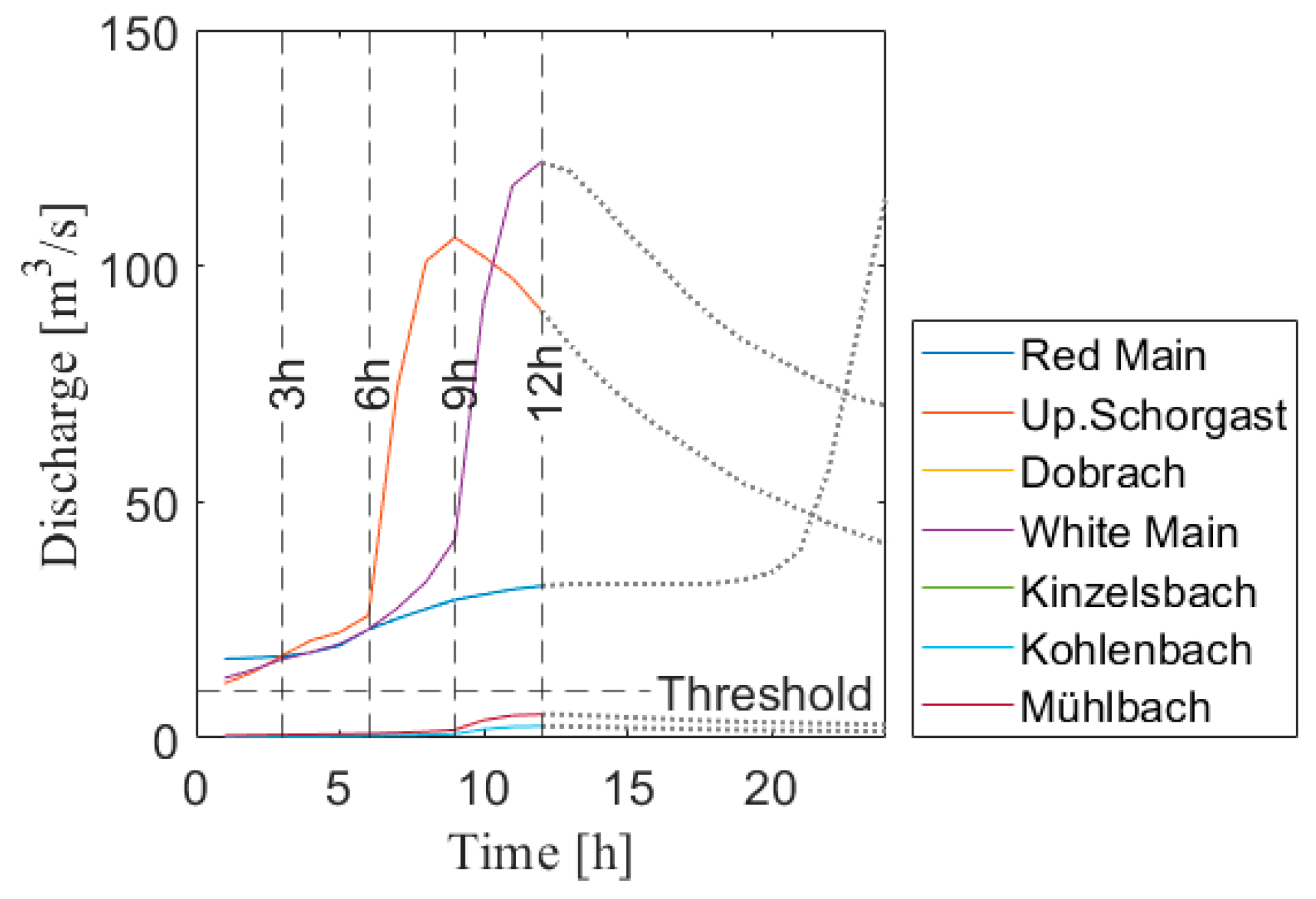
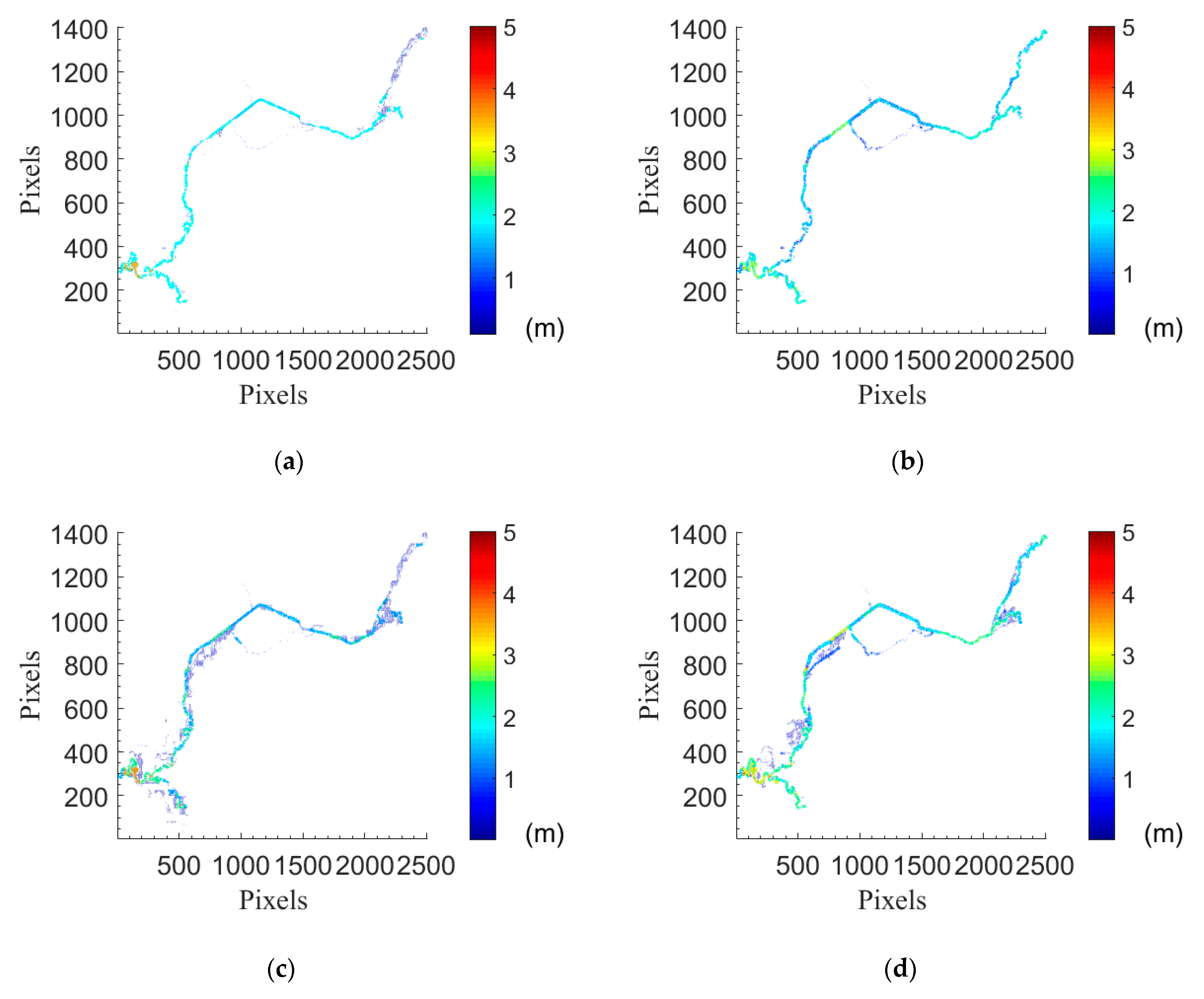
Figure 5 shows the discharge inputs for the historical flood event in 2006. The first 3 h, 6 h, 9 h, 12 h discharge curves are given by the trained ANN as in Chapter 4.1. Figure 6 compares the prediction of the inundation map of the first intervals of 3 h, 6 h, 9 h and 12 h with the inundation map from the hydraulic model of the historical flood event 2006.

Table 2. Numbers of wet grids and accurate grid percentage for event 2006. A wet grid is with the water level over 0.1 m; any water depth below this cutoff value is eliminated. Table shows grid numbers with a larger root-mean-square error (RMSE) and their percentages to the total wet grids.

Prediction Time (h)	Wet ANN Grid	ANN Grid with RMSE > 0.2 m	ANN Grid% with RMSE ≤ 0.2 m	ANN Grid with RMSE > 0.3 m	ANN Grid% with RMSE ≤ 0.3 m	ANN Grid with RMSE > 0.4 m	ANN Grid% with RMSE ≤ 0.4 m
3	280	46	83.57%	20	92.86%	6	97.86%
6	405	84	79.26%	42	89.63%	25	93.83%
9	474	134	71.73%	64	86.50%	36	92.41%
12	483	157	67.49%	85	82.40%	47	90.27%

Note: highlighted in gray are the percentages larger than 70%.

shows the performance of the prediction for historical event 2006, evaluated by average RMSE for each individual ANN. As the forecast interval increases from 3 h to 12 h, the prediction accuracy drops, evaluated by grid percentages of RMSE.

Historical flood events 2013

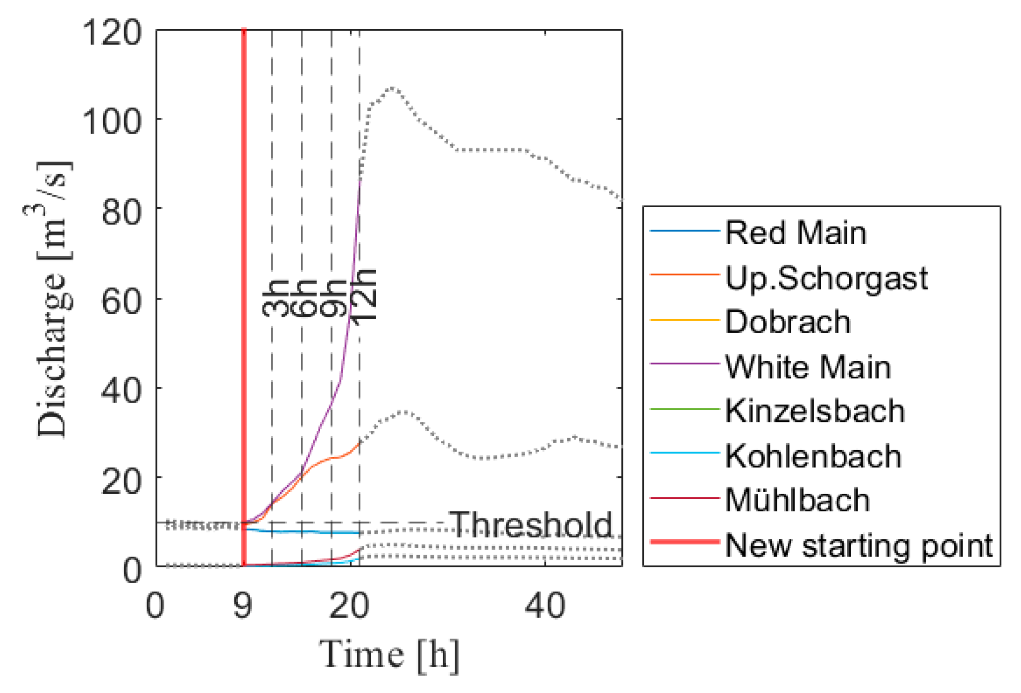
Figure 7 shows the discharge inputs for the historical flood event in 2013. It shows that the initial discharge curves are below the forecast threshold 10 m³/s; therefore, the start of the prediction at 9 h is marked with a red line when one discharge hits the forecast threshold. Figure 8 compares the prediction of the inundation map of the first intervals of 3 h, 6 h, 9 h and 12 h with the inundation map from the hydraulic model of the historical flood event 2013.

Table 3. Numbers of wet grids and accurate grid percentages for the flood event in 2013. A wet grid is with the water level over 0.1 m; any water depth below this cutoff value is eliminated. The table shows grid numbers with larger RMSE and their percentages to the total wet grids.

Prediction Time (h)	Wet ANN Grid	ANN Grid with RMSE > 0.2 m	ANN Grid% with RMSE ≤ 0.2 m	ANN Grid with RMSE > 0.3 m	ANN Grid% with RMSE ≤ 0.3 m	ANN Grid with RMSE > 0.4 m	ANN Grid% with RMSE ≤ 0.4 m
3	285	9	96.84%	2	99.30%	2	99.30%
6	405	72	82.22%	27	93.33%	8	98.02%
9	474	134	71.73%	65	86.29%	25	94.73%
12	483	175	63.77%	104	78.47%	56	88.41%

Note: highlighted in gray are the percentages larger than 70%.

shows the performance of the prediction for historical event 2013, evaluated by average RMSE for each individual ANN. The forecast performance is slightly better than that of the event 2006.

Historical flood events 2005

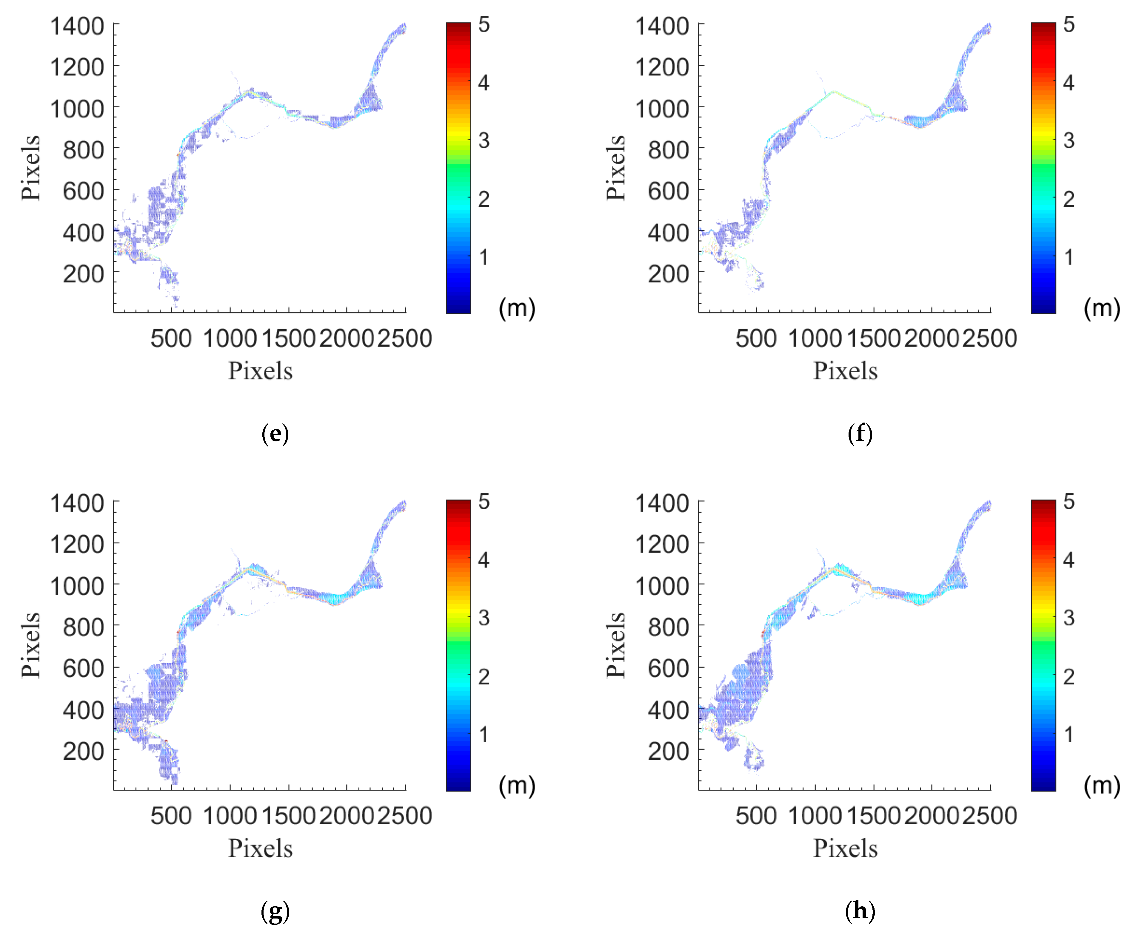
Figure 9 shows the discharge inputs for the historical flood event in 2005. Figure 10 compares the prediction of the inundation map of the first intervals of 3 h, 6 h, 9 h and 12 h with the inundation map from the hydraulic model of the historical flood event 2005.

Table 4. Numbers of wet grids and accurate grid percentages for the flood event in 2005. A wet grid is with the water level over 0.1 m; any water depth below this cutoff value is eliminated. Table shows grid numbers with larger RMSE and their percentages to the total wet grids.

Prediction Time (h)	Wet ANN Grid	ANN Grid with RMSE > 0.2 m	ANN Grid% with RMSE ≤ 0.2 m	ANN Grid with RMSE > 0.3 m	ANN Grid% with RMSE ≤ 0.3 m	ANN Grid with RMSE > 0.4 m	ANN Grid% with RMSE ≤ 0.4 m
3	280	65	76.79%	36	87.14%	19	93.21%
6	405	165	59.26%	115	71.60%	74	81.73%
9	474	216	54.43%	148	68.78%	93	80.38%
12	483	244	49.48%	168	65.22%	107	77.85%

Note: highlighted in gray are the percentages larger than 70%.

shows the prediction performance of historical event 2005, evaluated by average RMSE for each individual ANN. As the forecast interval increases from 3 h to 12 h, the prediction accuracy drops. This can be evaluated by the grid percentage of RMSE.

4.2. Assessment of Real-time Forecasting of Water Depths for Multistep Flood Forecast Intervals, 1–5 h

Historical flood events 2006

Table 5. Forecast accuracy percentages for the flood event in 2006. This table shows the grid percentage to the total wet grids with average RMSE within 0.3 m. The forecast begins by the starting point, several hours later than the event beginning for the real-time forecast.

Starting Point (h)	Prediction Interval (h)
	3	6	9	12
+1	98.93%	92.10%	83.12%	79.09%
+2	98.94%	90.86%	77.85%	79.92%
+3	96.94%	89.38%	76.58%	78.26%
+4	95.11%	86.95%	70.89%	75.36%
+5	86.60%	69.29%	66.88%	68.12%

Note: highlighted in gray are the percentages larger than 70%.

shows the forecast for multistep forecast intervals of the event in 2006. The forecast for the event in 2006 has good accuracy for all the intervals.

Historical flood events 2013

Table 6. Forecast accuracy percentages rate for the flood event in 2013. This table shows the grid percentage to the total wet grids with average RMSE within 0.3 m. The forecast begins by the starting point, several hours later than the event beginning for the real-time forecast.

Starting Point (h)	Prediction Interval (h)
	3	6	9	12
+1	99.30%	92.59%	84.18%	72.67%
+2	98.95%	89.88%	78.90%	70.39%
+3	96.30%	89.17%	75.74%	67.91%
+4	94.17%	82.51%	68.78%	67.29%
+5	91.28%	77.34%	66.46%	66.67%

Note: highlighted in gray are the percentages larger than 70%.

shows the forecast for multistep forecast intervals of the event in 2013. The forecast of the event in 2013 has good accuracy for all the intervals, with a similar performance as that of the event in 2006.

Historical flood event 2005

Table 7. Forecast accuracy percentages for the flood event in 2005. This table shows the grid percentages to the total wet grids with average RMSE within 0.3 m. The forecast begins by the starting point, several hours later than the event beginning for the real-time forecast.

Starting Point (h)	Prediction Interval (h)
	3	6	9	12
+1	83.74%	69.95%	66.89%	63.15%
+2	81.67%	68.23%	64.77%	61.70%
+3	76.31%	67.00%	63.08%	60.25%
+4	74.85%	66.50%	60.97%	60.25%
+5	70.97%	61.08%	58.65%	60.25%

Note: highlighted in gray are the percentages larger than 70%.

shows the forecast of multistep forecast intervals of the event 2005. The 3 h forecast of event 2005 still has a good accuracy of over 70%. For the 6 h, 9 h, 12 h forecasts, the ANN model produces less accurate results.

4.3. Forecast of the Inundation Extent

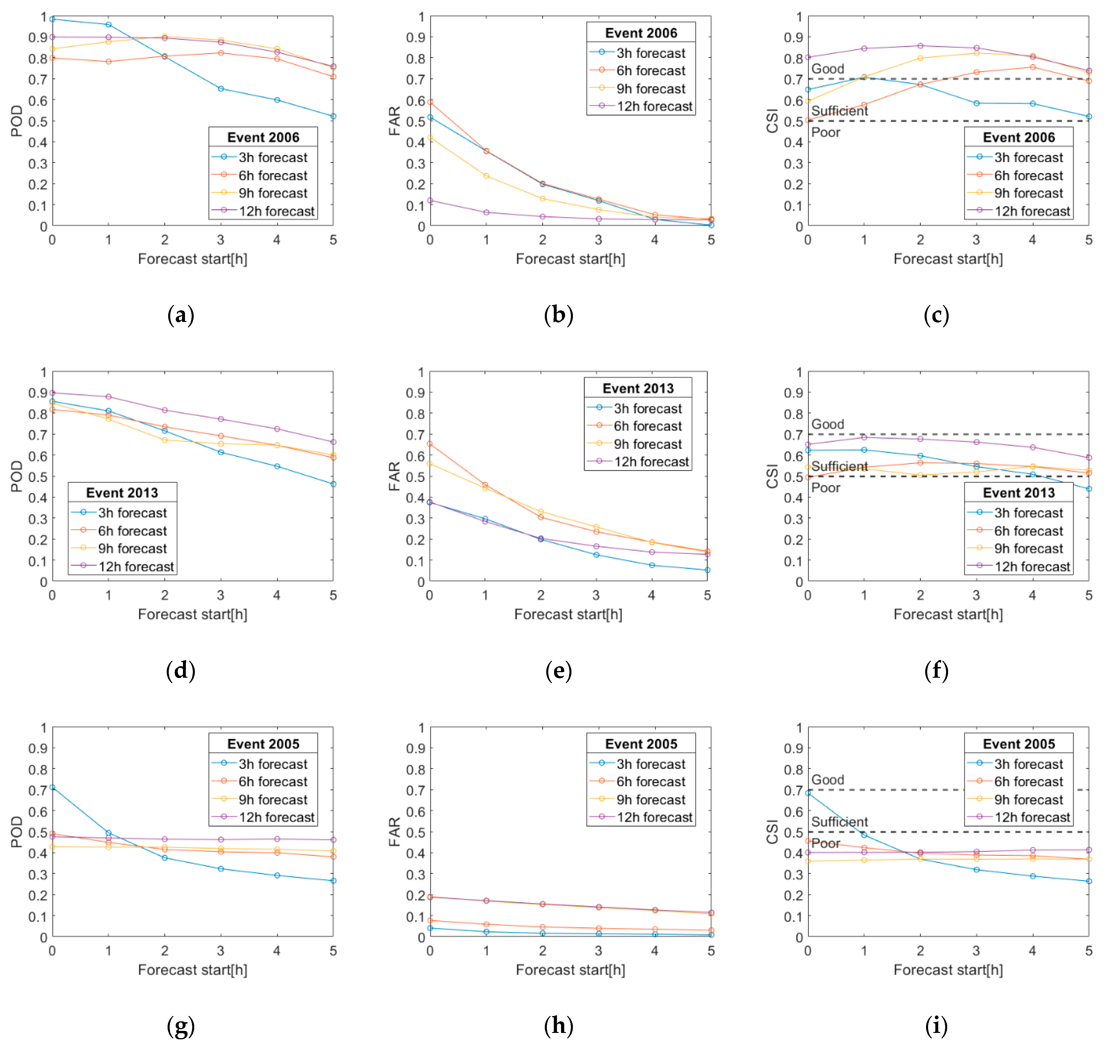
Figure 11 evaluates the ANN performance of the forecast of inundation extent (water depths over 0.1 m) growth with three indices. The status of wet/dry is used for calculating the following three indices for the likelihood between ANN and the hydraulic model. The probability of detection (POD) represents how well the ANN forecasted the same inundation extent as the hydraulic model. The false alarm ratio (FAR) measures the discrepancy of the ANN forecast to the hydraulic model. The critical success index (CSI) is the ratio between the correct forecasted inundation and the join of both the inundations (hits + misses + false alarms), showing the general correctness of the flood extent forecast of the ANN model. According to the verification criteria in another study [36], CSI over 0.7 (see Figure 11) is considered a good fit for the benchmark and over 0.5 (see Figure 11) is a sufficient fit. The lines in the figures show how these three indices change when a specific ANN is performed as the multistep forecasts advance in time.

5. Discussion

5.1. Assessment of the Prediction of Water Depths of the First Intervals of Flood Events

5.1.1. Synthetic Flood Events

Overall, the performance of the prediction of the first intervals of flood events shows that more than 80% of the grids have errors smaller than 0.3 m. The accuracy table (see Table 1) shows that the ANN has good accuracy in the water depth prediction of first intervals for all the synthetic events in the testing dataset. This test validated the network structure as well as the resilient backpropagation for solving the ANN. Since the network is initially trained with the 120 events from the synthetic event database and validated with the rest 60 events. The training events and the validation events bear more similarities with each other, which could explain the good performance of the prediction of the first interval of the ANN.

5.1.2. Historical Flood Events

Historical flood event 2006

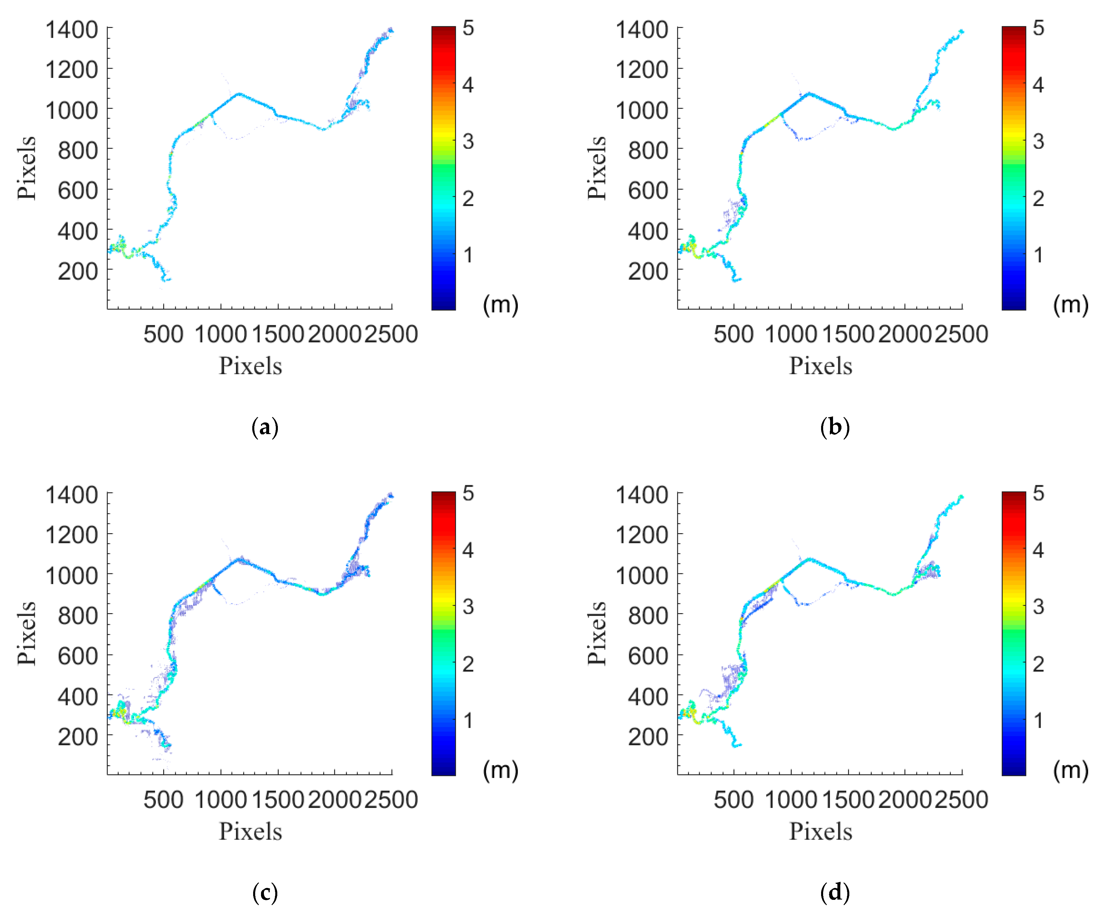
From Table 2, 83% of grids have RMSE smaller than 0.2 m, and the rest of the grids have RMSE around zero in 3 h prediction. For the 6 h prediction, 79% of grids have RMSE less than 0.2 m. In the 9 h and 12 h prediction, the area with large errors grows slightly (see Table 2). From Figure 6, the inundation maps from 3 h and 6 h predictions match well with the hydraulic inundation maps. The 9 h and 12 h are less accurate, especially in the southwest of the study area, which is further away from the location of the discharge inflows and is, thus, likely less sensitive to the changes in the discharge inputs. In brief, all the prediction for flood event 2006 is precise with more than 82% grids having RMSE less than 0.3 m.

Historical flood event 2013

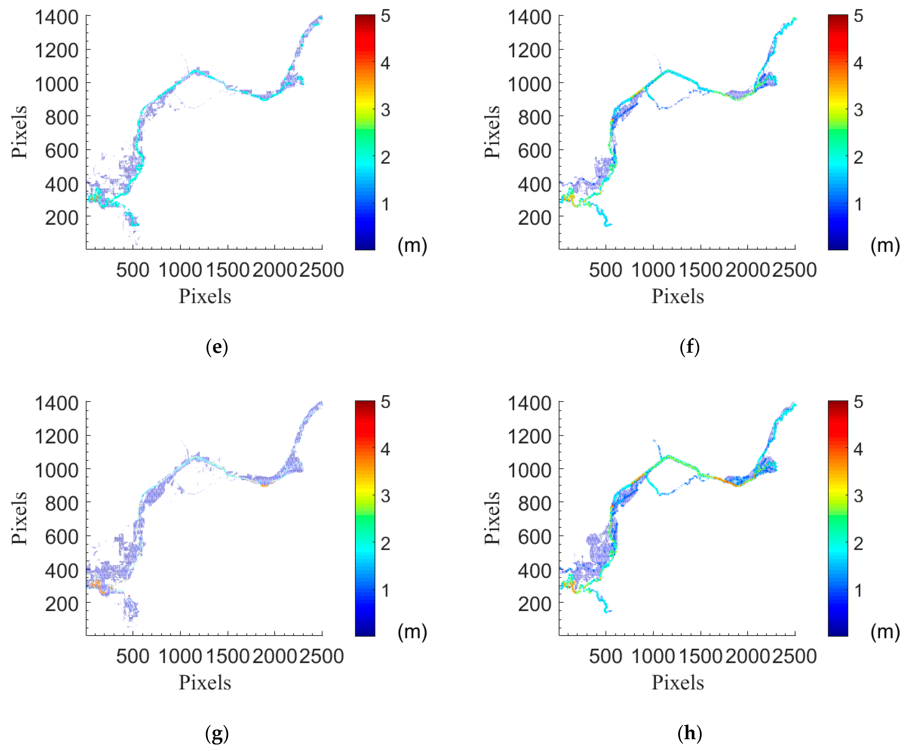
For the historical flood event 2013, the discharge forecast threshold for the forecast start was reached later, signaling that the discharge forecast threshold is indeed effective in starting and stopping the forecast. Therefore, the start of the forecast is picked up at a later moment in time once one discharge crosses the forecast threshold of 10 m³/s for a second time. The red line in Figure 7 marks the new start of the forecast (red line). For this event, it is nine hours later after the first forecast signaled by the ANN. Table 3 shows that the ANN model achieved high accuracy for the flood event in 2013. For the 3 h prediction, 96% of the grids have RMSE less than 0.2 m. 6 h prediction has 82% grids with RMSE less than 0.2 m. From 3 h and 6 h prediction of event 2013, the ANN performs better than the event 2006. Overall, the event of 2013 is also well predicted, with over 78% of grids having RMSE less than 0.3 m. Similar to event 2006, the predicted flood inundation maps of 3 h and 6 h intervals are similar to the hydraulic inundation simulations (see Figure 10).

Historical flood event 2005

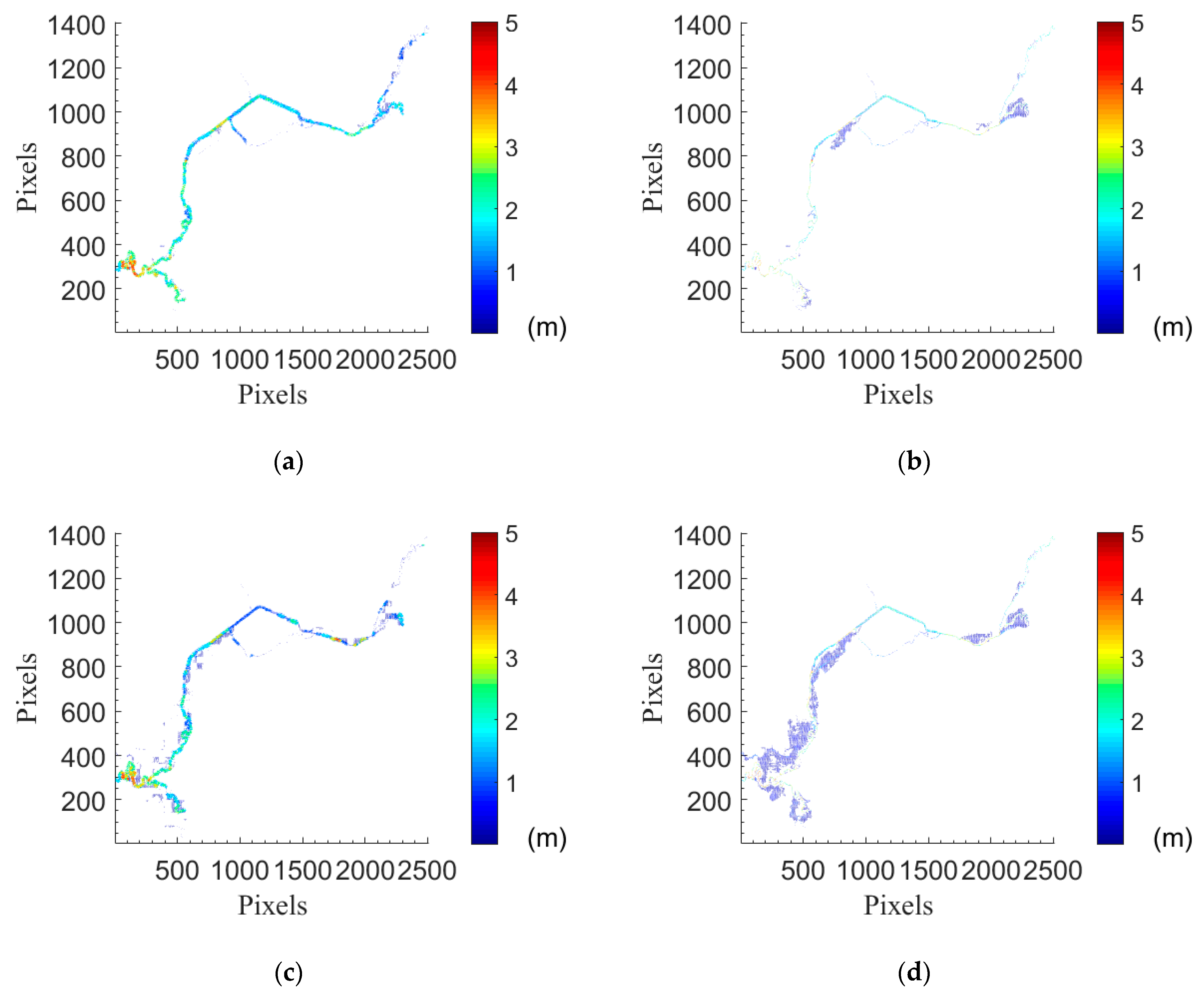
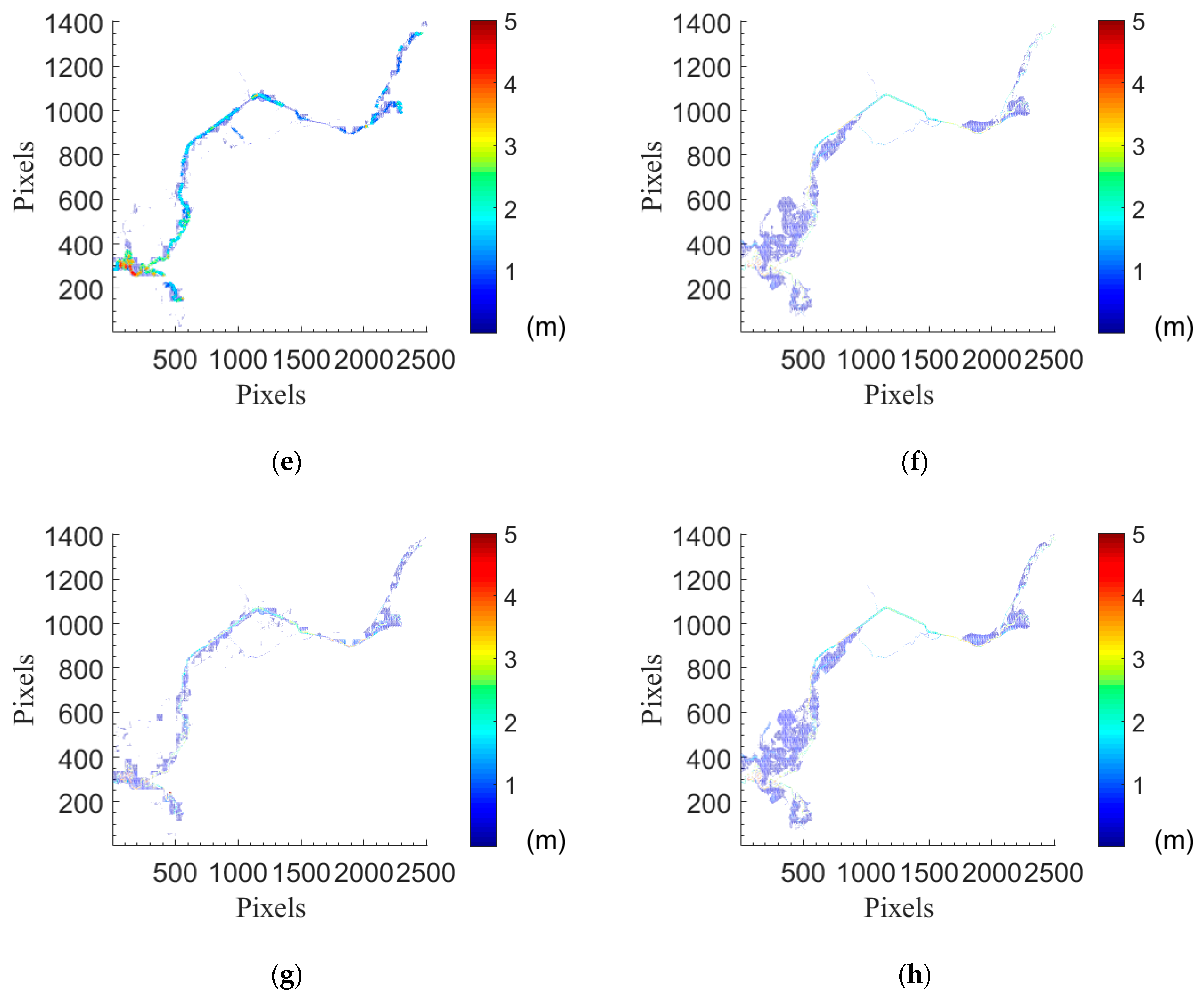
The general model performance for this flood event is less good. Figure 10 shows the comparison between the predicted inundation maps of ANN, where the inundated area is underestimated, compared to the hydraulic model (see the dark blue area in Figure 10b,d,f,h. However, Table 4 shows the prediction accuracy is still sufficient (above 65%) considering as acceptable an error within 0.3 m for the prediction of the first intervals for flood event 2005. The comparison can be observed in the water depth maps in Figure 6, Figure 8 and Figure 10, particularly when comparing the subplots (e) with (f) and (g) with (h). The ANN results differ more from the hydraulic results at points located closer to the southwest end of the study area. Reason being that those are the points that are further away from the inflow points (Figure 4).

5.2. Assessment of Real-time Forecasting of Water Depths for Multistep Flood Forecast Intervals, 1–5 h

In this section, we investigate if we can train different ANNs for the first interval of the forecast (from time 0) to predict the multistep forecast, the hypothesis of this study. Herein we test the ANN for four forecast intervals, namely for the next 3, 6, 9, 12 hours (X), and for five forecast starts 1–5 hours (S). This is represented by the format “X h + S”.

Historical flood event 2006

Table 5 shows the forecast accuracy of the historical flood event in 2006. The forecast of the 2006 flood event shows a good accuracy in 3 h, 6 h and most of 9 h (over 70% grid with RMSE < 0.3 m). It is visible that as the multistep forecast shifts further away from the original start used for the model training (X h + 5 h forecasts in Table 5), the ANN model performance decreases.

Historical flood event 2013

The discharge forecast threshold of the flood event from 2013 exceeds shortly at the beginning. Hence, the forecast is deactivated and reactivated again when the discharge exceeds the forecast threshold of 10 m³/s for the second time, namely 9 hours after time 0 (the first time the forecast window was activated). From the second starting point, all other forecasts are done for every forecast for X h + 1 h to X h + 5 h. Table 6 shows the forecast accuracy of the historical flood event of 2013. From this table, the ANN model performs as similar to the flood event in 2006. The forecast of the 2013 flood event has good results in 3 h, 6 h and most of 9 h (over 70% of the grid with RMSE < 0.3 m).

Historical flood event 2005

Table 7 shows the accuracy percentage of the grids evaluated by the RMSE less than 0.3 m. With the changing of the forecast starting point, all the forecasts of different intervals have similar RMSE as the forecast done during the first intervals. It is noticeable that the model provides a good forecast (over 70% grids with RMSE < 0.3 m) for 3 h intervals for all starting points. This shows that 3 h ANN trained for the first interval could be used to forecast subsequent intervals with a slight drop in the overall accuracy. However, the forecasts of 6 h, 9 h and 12 h show a poor performance (Table 5, Table 6 and Table 7). Similar to the other events, most of the errors occur in the southwest of the study area (Figure 10). However, in this particular event, the errors are substantially larger at the southwest than at the city center, hence the overall poor performance of the ANNs.

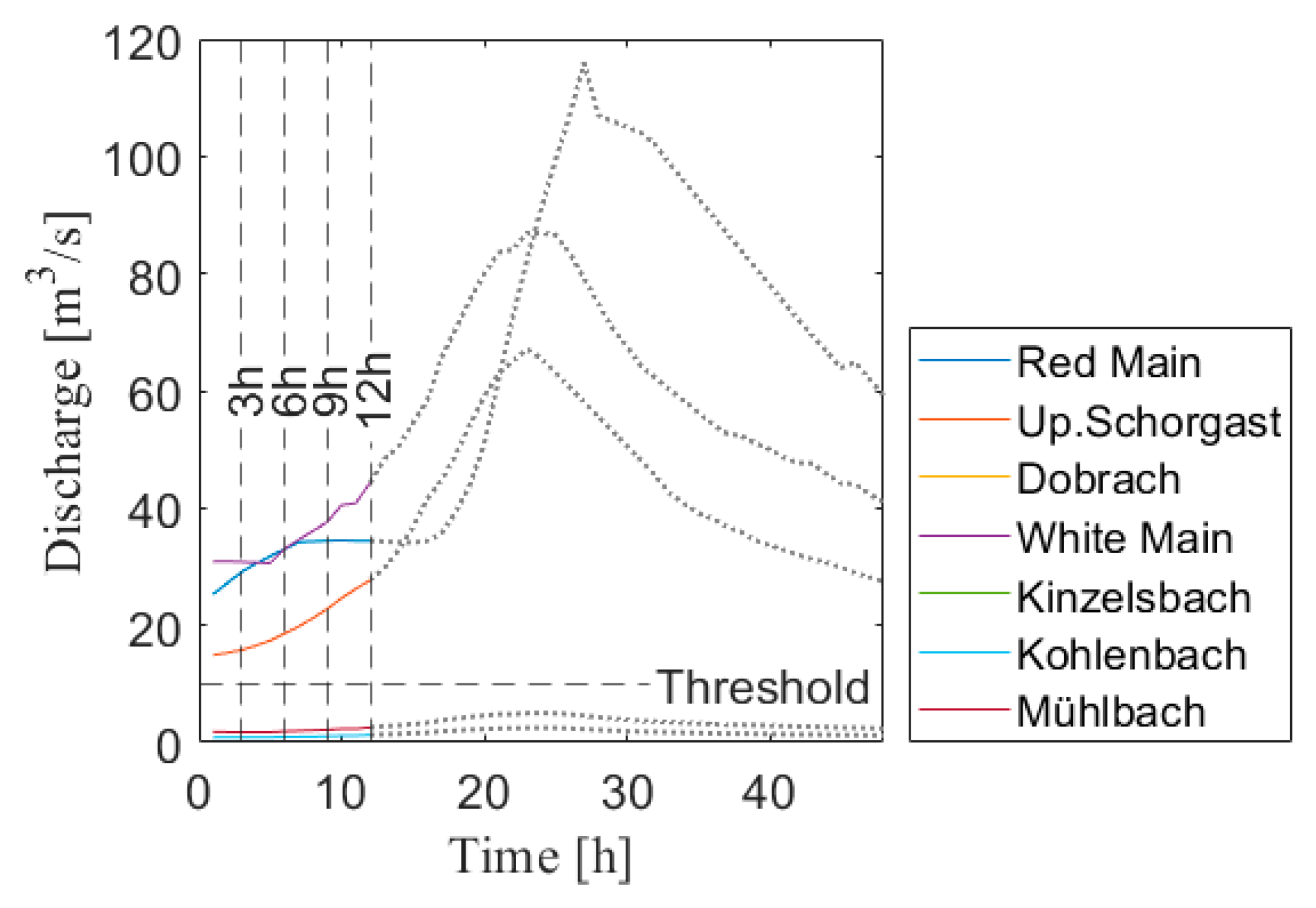
In all the three historical events, the forecast accuracy decreases as the forecast interval increases from 3 h to 12 h (see Table 5, Table 6 and Table 7). One exception occurs in the event 2006 between 9 h and 12 h, where the 12 h forecast has higher accuracy than the 9 h forecast. From the discharge curve (see Figure 5), unlike in other events, the two major discharges are falling after the peak value, which could be the reason for the higher accuracy at 12 h in this case.

5.3. Forecast of the Inundation Extent

The forecasts of flood inundation extent growths are examined through the statistical analysis proposed by Li et al. [33]. Figure 11 shows three indices, POD, FAR and CSI, for measuring the forecast performance of the flood inundation extent. Analyzing the POD index (see Figure 11a,d,g), it is clear that for the 3 h ANN forecast, the accuracy decreases slightly as forecasts proceeds from 3 h + 0 h to 3 h + 5 h. In other words, the accuracy of the 3 h ANN network is more sensitive to the shift of the forecast intervals than the 6 h, 9 h and 12 h ANN networks. The 3 h network achieves the best forecast performance for the first interval (training interval same as the forecast intervals). When moving forward for multistep forecast, shifting each hour decreases the POD by a value that varies between 0.08 to 0.1. This means that an added 8% to 10% of the inundation extent displayed by the hydraulic model is missing in the ANN forecast. In any case, and except for the event of 2005, the POD exhibits values above 70% for the first 2 hours of the forecast.

The FAR index (see Figure 11b,e,h) indicates the false-alarm percentage of the ANN forecasted flood inundation extents. In all three events, it is noticeable that the area percentage with false-alarms decreases over all the forecast networks when the forecast interval moves forward. It shows the ANN forecast produces more percentage of false alarms at the early stage in a flood event. This is because the flood inundation is relatively small at the beginning and the number of outer pixels larger than that of inner pixels, causing a higher number of false alarms. Moreover, the decreasing trend of POD and FAR indicate that the ANN model tends to change from overestimation to underestimation when the forecast starts to shift from 0–5 h.

The CSI index (see Figure 11c,f,i) shows the percentage of agreement of the ANN forecasts of the flood inundation extent to the hydraulic model. The ANN predicts better the flood inundation extents for two events of 2006 and 2013 than for the event of 2005, with the CSIs from 2006 and 2013 close to 0.6. For the event of 2005, the CSI is around 0.4 showing a poor accuracy forecast in the flood inundation extent forecast.

It is noteworthy to mention that the ANN shows an expectable performance of water depth prediction decreasing with lead time (see Table 5, Table 6 and Table 7). However, if we focus on the inundation extent, it seems contradictory, as the 12 h prediction shows better performance (see CSI and POD in Figure 11). The latter apparent contraction can be explained by the flood inundation extent being limited by the topography. The topography limits the size of the inundation, making it easier for the ANN to predict it better.

6. Conclusions

The aim of this study is to perform multiple subsequent forecasts for 1–5 h after the flooding event has started. It was shown that it is possible to use different ANNs for the first interval of the forecast (time 0) to issue the multistep forecasts. However, there should be made a distinction between the quality of the forecast regarding the water-depths or the flood inundation extent. The overall forecast performance of the water-depths was found slightly better than the flood inundation extents. The performance was mostly adversity affected by the flood event from 2005, in particular, close to the southwest end, far away from the location where the input inflows are.

The ANN model was first applied to the forecast of the first intervals of 3 h, 6 h, 9 h and 12 h. For the 60 synthetic flood events in the testing dataset, the model produced good results, as over 81% grids with RMSE less than 0.3 m. For the historical event 2006 and the historical event 2013, the model performed good water depths with the accuracy of over 82% and 78%, evaluated by RMSE smaller than the error threshold of 0.3 m. The flood event 2005 has a sufficient performance with an accuracy of over 65%, evaluated by RMSE smaller than 0.3 m. The forecasted inundation maps by ANN of all the three historical events have a similar shape to the inundation maps from the hydrodynamic model (HEC-RAS). For the far end area away from the inflow inputs, the long-distance may be responsible for a decrease in the forecast performance; therefore, it is likely that the model requires other information than those of discharge to enhance the forecast accuracy for those areas.

The ANN model was applied for the real-time forecast of the historical events in 2006, 2013 and 2005. For this purpose, the same ANN model was used for the forecast. The input discharge inputs were replaced by the shifted intervals for 1–5 h after the event’s beginnings. The forecast shows good results in the flood events 2006 and 2013 for the real-time forecasts, with over 70% grids with RMSE less than 0.3 m. The forecast shows worse results in flood event 2005, with only over 58% grids with RMSE less than 0.3 m. Overall, the forecast accuracy drops as the forecast interval increased from 3 h to 12 h. The forecast accuracy also decreases as the forecast progresses forward from X h + 1 h to X h + 5 h. For all the three historical flood events, the 3 h forecast is classified as good, with more than 70% grids accurately forecasted. However, the quality of 6 h or longer intervals was more event dependent.

Based on the analysis of indices of POD, FAR and CSI, the multistep ANN flood forecast provides good results at the beginning and decreases as the forecast progresses. The forecasts of the ANN model switches from an overestimation to an underestimation when the forecast proceeds from 0 h to 5 h. In our case, except for the event 2005, the 3 h ANN trained by the first interval improved the performances slightly with the multistep forecast; the 6 h, 9 h and 12 h ANN trained by the first interval for multistep interval forecasts would have accuracies depending on the exact flood events.

Future research could include recurrent neural networks with long short-term memory to involve the water depth information acquired from previous forecasted steps for a multistep forecast. To reduce the forecasted time interval for finer temporal multisteps could also be another possibility to enhance the accuracy of the forecast.

References

- Berz, G. Flood disasters: Lessons from the past-worries for the future. Water Manag. 2001, 148, 57–58. [Google Scholar] [CrossRef]
- Chang, L.C.; Amin, M.Z.M.; Yang, S.N.; Chang, F.J. Building ANN-based regional multi-step-ahead flood inundation forecast models. Water 2018, 10, 1283. [Google Scholar] [CrossRef] [Green Version]
- Henonin, J.; Russo, B.; Mark, O.; Gourbesville, P. Real-time urban flood forecasting and modelling—A state of the art. J. Hydroinform. 2013, 15, 717–736. [Google Scholar] [CrossRef]
- Hankin, B.; Waller, S.; Astle, G.; Kellagher, R. Mapping space for water: Screening for urban flash flooding. J. Flood Risk Manag. 2008, 1, 13–22. [Google Scholar] [CrossRef]
- Kalyanapu, A.J.; Shankar, S.; Pardyjak, E.R.; Judi, D.R.; Burian, S.J. Assessment of GPU computational enhancement to a 2D flood model. Environ. Model. Softw. 2011, 26, 1009–1016. [Google Scholar] [CrossRef]
- Mosavi, A.; Ozturk, P.; Chau, K.W. Flood prediction using machine learning models: Literature review. Water 2018, 10, 1–40. [Google Scholar]
- Dineva, A.; Várkonyi-Kóczy, A.R.; Tar, J.K. Fuzzy expert system for automatic wavelet shrinkage procedure selection for noise suppression. In Proceedings of the INES 2014 IEEE 18th Internationl Conference Intelligent Engineering Systems, Tihany, Hungary, 3–5 July 2014; pp. 163–168. [Google Scholar]
- Bermúdez, M.; Cea, L.; Puertas, J. A rapid flood inundation model for hazard mapping based on least squares support vector machine regression. J. Flood Risk Manag. 2019, 12, 1–14. [Google Scholar] [CrossRef] [Green Version]
- Gizaw, M.S.; Gan, T.Y. Regional Flood Frequency Analysis using Support Vector Regression under historical and future climate. J. Hydrol. 2016, 538, 387–398. [Google Scholar]
- Taherei Ghazvinei, P.; Darvishi, H.H.; Mosavi, A.; Bin Wan Yusof, K.; Alizamir, M.; Shamshirband, S.; Chau, K.W. Sugarcane growth prediction based on meteorological parameters using extreme learning machine and artificial neural network. Eng. Appl. Comput. Fluid Mech. 2018, 12, 738–749. [Google Scholar] [CrossRef] [Green Version]
- Noymanee, J.; Nikitin, N.O.; Kalyuzhnaya, A.V. Urban Pluvial Flood Forecasting using Open Data with Machine Learning Techniques in Pattani Basin. Procedia Comput. Sci. 2017, 119, 288–297. [Google Scholar] [CrossRef]
- Kasiviswanathan, K.S.; He, J.; Sudheer, K.P.; Tay, J.H. Potential application of wavelet neural network ensemble to forecast streamflow for flood management. J. Hydrol. 2016, 536, 161–173. [Google Scholar] [CrossRef]
- Zhang, G.P. Avoiding pitfalls in neural network research. IEEE Trans. Syst. Man Cybern. Part C Appl. Rev. 2007, 37, 3–16. [Google Scholar] [CrossRef]
- Dawson, C.W.; Wilby, R.L. Hydrological modelling using artificial neural networks. Prog. Phys. Geogr. 2001, 25, 80–108. [Google Scholar] [CrossRef]
- Yu, P.S.; Chen, S.T.; Chang, I.F. Support vector regression for real-time flood stage forecasting. J. Hydrol. 2006, 328, 704–716. [Google Scholar]
- Sit, M.; Demir, I. Decentralized flood forecasting using deep neural networks. arXiv 2019, arXiv:1902.02308. [Google Scholar]
- Bustami, R.; Bessaih, N.; Bong, C.; Suhaili, S. Artificial neural network for precipitation and water level predictions of bedup River. IAENG Int. J. Comput. Sci. 2007, 34, 228–233. [Google Scholar]
- French, J.; Mawdsley, R.; Fujiyama, T.; Achuthan, K. Combining machine learning with computational hydrodynamics for prediction of tidal surge inundation at estuarine ports. Procedia IUTAM 2017, 25, 28–35. [Google Scholar] [CrossRef]
- Berkhahn, S.; Fuchs, L.; Neuweiler, I. An ensemble neural network model for real-time prediction of urban floods. J. Hydrol. 2019, 575, 743–754. [Google Scholar] [CrossRef]
- Lin, Q.; Leandro, J.; Wu, W.; Bhola, P.; Disse, M. Prediction of Maximum Flood Inundation Extents with Resilient Backpropagation Neural Network: Case Study of Kulmbach. Front. Earth Sci. 2020, 8, 1–8. [Google Scholar]
- Shen, H.-Y.; Chang, L.-C. On-line multistep-ahead inundation depth forecasts by recurrent NARX networks. Hydrol. Earth Syst. Sci. Discuss. 2012, 9, 11999–12028. [Google Scholar] [CrossRef]
- Sit, M.; Demiray, B.Z.; Xiang, Z.; Ewing, G.J.; Sermet, Y.; Demir, I. A comprehensive review of deep learning applications in hydrology and water resources. Water Sci. Technol. 2020. [Google Scholar] [CrossRef]
- Nawi, N.; Ransing, R.; Ransing, M. An improved Conjugate Gradient based learning algorithm for back propagation neural networks. Int. J. Comput. Intell. 2007, 4, 46–55. [Google Scholar]
- Sankaranarayanan, S.; Prabhakar, M.; Satish, S.; Jain, P.; Ramprasad, A.; Krishnan, A. Flood prediction based on weather parameters using deep learning. J. Water Clim. Chang. 2019, 1–18. [Google Scholar] [CrossRef]
- Kohavi, R. A study of cross-validation and bootstrap for accuracy estimation and model selection. In Proceedings of the Appears in the International Joint Conference on Articial Intelligence (IJCAI), Stanford, CA, USA, 19 August 1995; Volume 8. [Google Scholar]
- Jhong, Y.D.; Chen, C.S.; Lin, H.P.; Chen, S.T. Physical hybrid neural network model to forecast typhoon floods. Water 2018, 10, 632. [Google Scholar] [CrossRef] [Green Version]
- Wang, H.; Rahnamayan, S.; Wu, Z. Parallel differential evolution with self-adapting control parameters and generalized opposition-based learning for solving high-dimensional optimization problems. J. Parallel Distrib. Comput. 2013, 73, 62–73. [Google Scholar] [CrossRef]
- Kabir, S.; Patidar, S.; Xia, X.; Liang, Q.; Neal, J.; Pender, G. A deep convolutional neural network model for rapid prediction of fluvial flood inundation. J. Hydrol. 2020, 590, 125481. [Google Scholar] [CrossRef]
- Saini, L.M. Peak load forecasting using Bayesian regularization, Resilient and adaptive backpropagation learning based artificial neural networks. Electr. Power Syst. Res. 2008, 78, 1302–1310. [Google Scholar] [CrossRef]
- Panda, R.K.; Pramanik, N.; Bala, B. Simulation of river stage using artificial neural network and MIKE 11 hydrodynamic model. Comput. Geosci. 2010, 36, 735–745. [Google Scholar] [CrossRef]
- Bhola, P.K.; Leandro, J.; Disse, M. Framework for offline flood inundation forecasts for two-dimensional hydrodynamic models. Geosciences 2018, 8, 346. [Google Scholar] [CrossRef] [Green Version]
- Bhola, P.K.; Nair, B.B.; Leandro, J.; Rao, S.N.; Disse, M. Flood inundation forecasts using validation data generated with the assistance of computer vision. J. Hydroinform. 2019, 21, 240–256. [Google Scholar] [CrossRef] [Green Version]
- Li, L.; Hong, Y.; Wang, J.; Adler, R.F.; Policelli, F.S.; Habib, S.; Irwn, D.; Korme, T.; Okello, L. Evaluation of the real-time TRMM-based multi-satellite precipitation analysis for an operational flood prediction system in Nzoia Basin, Lake Victoria, Africa. Nat. Hazards 2009, 50, 109–123. [Google Scholar] [CrossRef]
- Ludwig, K. The Water Balance Model LARSIM: Design, Content and Applications, Freiburger Schriften zur Hydrologie. Master’s Thesis, Institut für Hydrologie der University, Hannover, Germany, 2006. [Google Scholar]
- Hochwassernachrichtendienst Bayern, added level data (MQ) from water level Ködnitz/White Main. Available online: www.hnd.bayern.de (accessed on 12 December 2019).
- Bernhofen, M.V.; Whyman, C.; Trigg, M.A.; Sleigh, P.A.; Smith, A.M.; Sampson, C.C.; Yamazaki, D.; Ward, P.J.; Rudari, R.; Pappenberger, F.; et al. A first collective validation of global fluvial flood models for major floods in Nigeria and Mozambique. Environ. Res. Lett. 2018, 13. [Google Scholar] [CrossRef] [Green Version]
Figure 1.
The forward-feed neural network setup in the forecast study. The input layer is fed with discharge inflows of certain time interval windows. The output layer generates the flood inundation for that interval. Resilient backpropagation is applied for training this network.
Figure 2.
Training of artificial neural networks (ANN) forecast model. Four ANN models for 3 h, 6 h, 9 h, 12 h first interval predictions are set up in this work, trained with the discharges from each synthetic flood event. After this, the models are to predict the corresponding first intervals for other events.
Figure 3.
Shift of ANN forecast models for multistep forecast intervals. The yellow color shows the forecast of the first interval (forecast interval same as the training interval, i.e., at time 0). The green color shows applying the original 3 h forecast network for 1 h later forecast from 1–4 h. The orange color shows applying the original 3 h forecast network for 2 h later forecast from 2–5 h. The black box shows the general case of applying the original X h forecast network for S h later forecast, from S h to X h + S.
Figure 4.
Map of the study area. It shows the location of Kulmbach in Germany. The blue curves represent the river network. The shaded region is the study area with its topography represented. On the marked boundary, the red points represent the seven inflows on the boundary (three rivers and four smaller streams).
Figure 5.
Hydrographs of the flood event in 2006. Seven discharge curves of three rivers and four streams are shown in different colors. Time 0 marks the start of the prediction. The dash lines upon the discharge curves mark the different discharge sections for prediction inputs.
Figure 6.
Inundation maps from the prediction of water depths of the first intervals in flood event 2006. (a) ANN inundation map 3 h; (b) hydrodynamic inundation map 3 h; (c) ANN inundation map 6 h; (d) hydrodynamic inundation map 6 h; (e) ANN inundation map 9 h; (f) hydrodynamic inundation map 9 h; (g) ANN inundation map 12 h; (h) hydrodynamic inundation map 12 h.
Figure 7.
Hydrographs of the flood event in 2013. Seven discharge curves of three rivers and four streams are shown in different colors. The red line time marks the new start of the prediction at 9 h, where one discharge first exceeds the forecast threshold of 10 m3/s. The dash lines upon the discharge curves mark the different discharge sections for prediction inputs.
Figure 8.
Inundation maps from the prediction of water depths of the first intervals in flood event 2013. (a) ANN inundation map 3 h; (b) hydrodynamic inundation map 3 h; (c) ANN inundation map 6 h; (d) hydrodynamic inundation map 6 h; (e) ANN inundation map 9 h; (f) hydrodynamic inundation map 9 h; (g) ANN inundation map 12 h; (h) hydrodynamic inundation map 12 h.
Figure 9.
Hydrographs of the flood event in 2005. Seven discharge curves of three rivers and four streams are shown in different colors. Time 0 marks the start of the prediction. The dash lines upon the discharge curves mark the different discharge sections for prediction inputs.
Figure 10.
Inundation maps from the prediction of water depths of the first intervals in flood event 2005. (a) ANN inundation map 3 h; (b) hydrodynamic inundation map 3 h; (c) ANN inundation map 6 h; (d) hydrodynamic inundation map 6 h; (e) ANN inundation map 9 h; (f) hydrodynamic inundation map 9 h; (g) ANN inundation map 12 h; (h) hydrodynamic inundation map 12 h.
Figure 11.
Performance of the forecast of inundation extent growths by three indices. (a) probability of detection (POD) in flood event 2006; (b) false alarm ratio (FAR) in flood event 2006; (c) critical success index (CSI) in the flood event 2006; (d) POD in flood event 2013; (e) FAR in the flood event 2013; (f) CSI in flood event 2013; (g) POD in flood event 2005; (h) FAR in flood event 2005; (i) CSI in flood event 2005.