Settling of Road-Deposited Sediment: Influence of Particle Density, Shape, Low Temperatures, and Deicing Salt


1
Chair of Urban Water Systems Engineering, Technical University of Munich, Am Coulombwall 3, 85748 Garching, Germany
2
Fachgebiet Siedlungswasserwirtschaft und Hydromechanik (Institute of Urban Water Management and Hydromechanics), Frankfurt University of Applied Sciences, Nibelungenplatz 1, 60318 Frankfurt am Main, Germany
*
Author to whom correspondence should be addressed.
Water 2020, 12(11), 3126; https://doi.org/10.3390/w12113126
Submission received: 7 October 2020
/
Revised: 2 November 2020
/
Accepted: 5 November 2020
/
Published: 7 November 2020
(This article belongs to the Special Issue Rainwater Management in Urban Areas)
Abstract
:Separation of particulate matter (PM) is the most important process to achieve a reduction of contaminants present in road runoff. To further improve knowledge about influencing factors on the settling of road-deposited sediment (RDS), samples from three sites were collected. Since particle size distribution (PSD) has the strongest effect on settling, the samples were sieved to achieve comparable PSDs so that the effects of particle density, shape, fluid temperature, and deicing salt concentration on settling could be assessed using settling experiments. Based on the experimental data, a previously proposed model that describes the settling of PM was further developed and validated. In addition, RDS samples were compared to a standard mineral material, which is currently in use to evaluate treatment efficiency of stormwater quality improvement devices. The main finding was that besides PSD, particle density is the most important influencing factor. Particle shape was thoroughly described but showed no significant improvement of the prediction of the settled mass. Temperature showed an effect on PM settling; deicing salts were negligible. The proposed models can sufficiently predict the settling of RDS in settling column experiments under varying boundary conditions and are easily applicable.
1. Introduction
Road-deposited sediment (RDS) is an important source of contamination in urban environments [1,2,3]. RDS contains inorganic and organic pollutants such as heavy metals (e.g., Cu, Zn, Pb, Cd, Cr, Ni) and polycyclic aromatic hydrocarbons (PAH) [4,5,6]. To mitigate the effect caused by RDS on the environment, stormwater control measures (SCMs) such as stormwater quality improvement devices (SQIDs) and detention basins are designed to retain RDS from stormwater runoff by sedimentation or filtration [7,8]. However, previous studies have shown that SCMs exhibit reduced retention efficiency under winter conditions caused by low temperature and deicing salts [9,10,11]. To design the sedimentation stages of SQIDs, knowledge about particle characteristics and settling velocity distributions of RDSs is crucial [12,13], especially to separate fine particles and particles with low density, which show an increased contaminant load [5,14,15,16,17]. In addition, the influence on settling by particle size distribution (PSD), particle density, and runoff event-specific properties, such as first flush and runoff volume and intensity, has been comprehensively studied [18,19,20,21,22,23]. Other factors such as temperature, deicing salt, and particle shape have not been sufficiently investigated yet.
The first predictions of Rommel and Helmreich [9] indicated that the presence of deicing salt (sodium chloride) had a negligible influence on the retention of particles. However, reducing the temperature from 20 to 5 °C was shown to decrease the removal efficiency of RDS in a sedimentation shaft by up to 8%. To calculate densities and viscosities of various deicing salt solutions, the equations of Laliberté [24,25] were adapted. The order of influencing factors for the sedimentation was found to be particle size distribution >> overflow rate > particle density > temperature. Even though the results of a 20-month monitoring of full-scale sedimentation indicated worse particulate matter (PM) separation in the cold season, the data were not sufficient to quantify the influencing factors. Thus, lab-scale experiments, with a comparable setup, would be necessary to exclude other environmental influences on the sedimentation, which are always present under real conditions (i.e., varying discharge rates and PM properties, stratification and mixing of water with different temperature and deicing salt concentrations), and validate the modeling predictions.
There are various protocols to determine settling velocity distribution [12,17,26,27,28]; however, they have not been utilized yet to quantify the influence of temperature and deicing salts on the settling velocity of RDSs. Commonly, artificial test materials are used to reduce variations of PM properties [17]. Gelhardt et al. [17] developed a laboratory method to measure and compare the settling behavior of artificial and real particle collectives with a reproducible PSD. Real RDSs were used in the study, yet the focus was on method development and not on the influence of boundary conditions on the settling behavior of RDS. Ying and Sansalone [29] were, to our best knowledge, the first authors who adapted settling experiments to study the effect of temperature and concentration of deicing salts on the settling of PM from urban runoff. They concluded—based on a computational fluid dynamics (CFDs) model of a hydrodynamic separator—that temperature and deicing salt is negligible to describe the discrete settling of PM.
As these results partly differ from the results of Rommel and Helmreich [9] and the investigation was done with the model of a hydrodynamic separator and not a basic sedimentation unit, the settling column experiments proposed by Gelhardt et al. [17] were adapted to further evaluate the effects of particle density, shape, temperature, and deicing salt (sodium chloride, NaCl) concentration. Based on these results, the model proposed by Rommel and Helmreich [9] was further developed to be able to model settling experiments and was consecutively validated.
Hence, RDSs were thoroughly characterized, and the effects of the influencing factors studied in settling column experiments. Furthermore, the nonspherical shape of RDS was evaluated using dynamic image analysis and considered in an additional model. Since the determination of particle sphericity is still difficult to measure for engineering purposes [30,31], sphericity was approximated by 2D projections of the particles captured using dynamic image analysis.
There exist recent studies that have determined the drag or settling velocity of irregular particles based on more complex descriptions of particle shapes [32,33,34]. However, our approach was to simplify the particle description and model so that it is more accessible for the engineering purposes of stormwater treatment. In addition, the standard mineral material, which is in use for the technical approval of SQIDs in Germany [35,36], was compared to RDSs.
2. Materials and Methods
2.1. Materials—Study Site and Characterization
Three RDS samples were collected using a vacuum cleaner (DCV 582, Dewalt Deutschland, Idstein, Germany) at three locations in Frankfurt, Germany, with varying annual average daily traffic (AADT) and land usage, which affects RDS properties (Table 1). Solids on the road surface were loosened by means of a paintbrush. In addition to the RDS, the standard mineral material MiW4 (Millisil W4, Quarzwerke, Haltern, Germany) was used for comparison to the RDSs. MiW4 is a milled quartz material, which is in use in the German technical approval procedure of SQIDs to assess PM separation efficiency. It reflects the PSD of road runoff [17,35]. Prior to sieving, the samples were dried at 105 °C until constant weight was achieved. Fractions > 2 mm were removed using a stainless steel sieve.
To achieve a comparable PSD of all studied RDS, the samples were sieved using a sieve stack with the mesh sizes 1000, 500, 250, 200, 160, 125, 100, 63, and 40 µm, respectively. Subsequently, the obtained fractions were again dried at 105 °C and merged with the percentages summarized in Table 2. The sieving process is described in detail in Gelhardt et al. [17].
The sieve fractions were characterized by measuring particle density ρs and the loss on ignition (LOI). The ρs was determined using a gas pycnometer (Quantachrome Microultrapyk 1200 eT, Anton Paar QuantaTec, Boynton Beach, USA) with helium (5.0, Air Liquide, Düsseldorf, Germany, Purity ≥ 99.999%), according to DIN 66137-2. To determine the LOI, the dried materials were ignited in a muffle furnace at 550 °C for 2 h (DIN EN 15169). LOI is an indicator to assess the organic fraction of the RDS. The characteristics of the studied materials are summarized in Table 1.
Particle size and shape were determined by dynamic image analysis according to ISO 13322-2 (2006) using the system QICPIC+LIXELL+LIQXI (Sympatec, Clausthal-Zellerfeld, Germany). The module M5 was used, with a measuring range between 1.8 and 3755 µm. Prior to the analysis, the samples were dispersed in deionized water using ultrasonic homogenization at 50% amplitude for 60 s (Sonopuls HD 2200.2, Bandelin, Berlin, Germany). Approximately 0.25 g of the sample was applied to 200 mL of deionized water to achieve an optimum concentration of < 2% during the measurement. Settings of the device were 800 U min−1 stirring rate, 125 U min−1 recirculation rate, 30 Hz frame rate, and 60 s acquisition time. These settings were optimized for the reproducibility of the PSD of MiW4. Data were analyzed using the proprietary software PAQXOS (Sympatec, Clausthal-Zellerfeld, Germany). Based on suggestions by the manufacturer of the device, particles <5.4 µm were discarded for size analysis and particles <16 µm were discarded for the shape analysis to assure sufficient image resolution. One million particles were analyzed for each sample due to the aforementioned thresholds; particle counts decreased. The following size and shape parameters were determined: the area equivalent circle diameter (deq); the Riley circularity [37], where is the diameter of the largest inscribed circle and is the smallest circumscribed circle; the aspect ratio , where is the minimal Feret diameter and .is the maximal Feret diameter (ISO 9276-6:2008). Values of φRiley > 1 were substituted by 1, since the value 1 would be the value of a circle and values >1 were caused by measuring uncertainties. Numerous other definitions of circularity exist; we selected φRiley because it was suggested by Bagheri et al. [38] as a predictor for particle sphericity. As the experiments were focused on the settled mass, size and shape distributions were weighted by the mass fractions of the particles. These were determined under the assumptions of constant density for each sample and a spherical particle shape with the diameter deq.
2.2. Settling Experiments
The settling experiment utilized in this study is based on the method proposed by Gelhardt et al. [17], which was adapted from the method, developed by the company UFT [28]. A comprehensive description can be found in Gelhardt et al. [17].
In the experiments, glass columns with a length of 780 mm and an inner diameter of 50 mm were used. The settling height was 760 mm. This method is a floating layer method [27]. Since this study did not intend to determine settling velocity distributions, only the settled fraction after 4 min was evaluated. This fraction exhibits a settling velocity of ≥ 11.4 m h−1, which approximately reflects the fraction ≥ 63 µm of mineral material with a density of 2.65 g cm−3.
Prior to each experiment, the columns filled with deionized water (DI water) were adjusted to either 21.0 ± 0.1 or 10.0 ± 0.1 °C in a climate chamber (Thermo-TEC, Rochlitz, Germany), depending on the experiment. Additional experiments with 20 g L−1 NaCl (VWR, p.A., CAS: 7647-14-5; wNaCl = 0.02) were performed to assess the influence of deicing salt at 10 °C. This NaCl concentration can be considered an extreme value for deicing salt concentration in road runoff [39,40]. The names of the experiments used in the remaining text consist of the following information: material, temperature and NaCl concentration (e.g., MiW4, 21 °C, 0 g/L).
Temperature and electrical conductivity (EC) were measured according to standard method 2510 B [41]. A suspension containing 0.5 g RDS or MiW4 was applied in the experiments. The suspension was prepared prior to the experiment in 15 mL glass vials by adding 10 mL of the same solution in the columns to the RDS or MiW4. The suspension was homogenized by 1 min of manual shaking. The settling experiments were conducted without delay after the preparation of the suspension. Thus, no alteration of the samples can be expected [18]. The sample of the settled fraction was withdrawn after 4 min. The mass of the settled fraction was determined after the evaporation of the withdrawn sample according to standard method 2540 B [41]. Since dissolved NaCl would severely bias the results, the samples of experiments with wNaCl > 0 were analyzed using membrane filtration with 0.45 µm membrane filters (cellulose nitrate, Sartorius, Type 113, 47 mm diameter) in accordance with standard method 2540 D [41]. Both methods for the determination of the settled fraction, either evaporation or filtration, were in good agreement with each other (cf. Figure S1). To determine the nonsettled fraction, the water remaining in the column after the experiment was filtered and the total suspended solids (TSS) were determined according to standard method 2510 B [41]. The lost particulate mass was calculated by the initial particulate mass subtracted by the sum of the settled and nonsettled particulate mass. In the experiments, 3.3% ± 1.9% of the particulate mass was lost; this was not considered in the determination of the settled mass fractions. Each experiment was conducted in triplicate.
2.3. Modeling of Settling Experiments
The entire model was implemented in Python with the packages Pandas, Matplotlib, SciPy, and Seaborn [42,43,44,45]. It is accessible in Supplementary Material A.
The PSD of the preprocessed RDSs were modeled using a Weibull cumulative probability density function [9,46,47], following Equation (1)
where W(d, λ, κ) = mass fraction less than d (-); d = particle diameter (μm); λ = shape parameter (-); κ = scale parameter (-) [9,46,47]. The determined λ and κ were 85.09 and 1.247 for the used PSD. These parameters were determined by the curve fitting in Matlab R2019a (MathWorks, Natick, USA) using the upper particle diameters of the fractions and nonlinear least squares method with the Trust-Region algorithm (R² = 0.998, RMSE = 0.016). The λ and κ are within the range of previously reported values for PSD in urban stormwater or RDS [9,47]. The PSD was described in the range of 0–250 µm, with 1-µm increments (Figure S2).
Density (), dynamic viscosity (), and kinematic viscosity () of the evaluated fluids at varying fluid temperatures (t) and NaCl mass fractions (wNaCl) were determined using the equations established by Laliberté et al. [24,25], as described in Rommel and Helmreich [9].
The terminal settling velocity (w) was determined by means of different approaches, with further consideration of influencing factors for each particle diameter (d), ρs, t, wNaCl, and sphericity (ϕ) for Model C. In addition, d was approximated by the Weibull fit of the PSD since the diameter of isotropic-shaped particles can be approximated by the screen size [48].
- Model A: Spherical particles
- Model B: Spherical particles with consideration of the withdrawn sample volume
- Model C: Nonspherical particles
The different models are explained in Section 2.3.1, Section 2.3.2 and Section 2.3.3. All models used the simplification of constant ρs (and ϕ for Model C) with respect to particle size. The models used the respective ρs and ϕ of the samples used in the experiments. Furthermore, they solely considered discrete settling without the interaction of the particles and no wall effect. Since the PSD was previously defined, a continuous settling velocity distribution was derived for each experiment.
To determine the mass of the settled fraction, the mass fraction at the critical settling velocity (wcrit) was calculated by linear interpolation. All settled particles exhibit a settling velocity greater or equal than wcrit. The settled mass fraction was determined by the difference of 1 and the mass fraction at wcrit.
2.3.1. Model A: Spherical Particles
Model A determined w (m s−1) using the explicit formulas (Equations (2)–(6)) proposed by Cheng [49] for spherical particles in the subcritical region ()
where is the dimensionless grain diameter, g is the gravitational acceleration (m s−2), CD is the drag coefficient (-), and is the dimensionless settling velocity [49]. Even if remains in the low region (< 10), this method avoids the necessity of checking Re during the calculation since it is valid for .
2.3.2. Model B: Spherical Particles with Consideration of the Withdrawn Sample Volume
Model B is based on Model A and additionally considers the withdrawn sample volume. Since additional water will be withdrawn with the sediment, not-yet-settled particles will be withdrawn as well. Thus, wcrit needs to be reduced with respect to the withdrawn sample volume. This was considered by reducing wcrit by the height of the truncated cone (hcone) with the same shape as the utilized glass columns and the volume of the withdrawn sample; hcone of each experiment was determined following Equation (7).
where Vsample is the measured withdrawn sample volume of each experiment in mL and hcone is the height of the truncated cone in cm. The determined was used to adjust wcrit to simulate the results of the experiments following Equation (8)
where wcrit is the critical settling velocity in m s−1, which is the minimal settling velocity of the particles-withdrawn sample after 4 min, and hcone the height of the truncated cone with the same shape as the utilized glass columns and the volume of the withdrawn sample in mL.
2.3.3. Model C: Nonspherical Particles
To consider the influence of a nonspherical particle shape, Model C included the average sphericity of each RDS determined by dynamic image analysis. Since dynamic image analysis only delivers 2D projections of the particles, the sphericity of the particles () was approximated by the circularity of the 2D projections of the particles, as proposed by Bagheri et al. [38]. Settling velocity of the nonspherical particles was predicted using the formulas proposed by Haider and Levenspiel [48] (Equations (9)–(11)) since it is an explicit and simple solution. Furthermore, it shows an acceptable average error [50].
where ϕ was approximated by the circularity of the 2D projections of the particles [30,38]. Bagheri et al. [38] suggested the use of φRiley for particles with a nonvesicular surface. Based on dynamic image analysis, the particles of the analyzed RDSs showed a nonvesicular surface; thus, the mass fraction weighted median of φRiley was used to approximateϕ.
2.4. Statistics
All statistical methods were implemented using Python with the packages Pandas 1.0.5 [43], Scipy 1.5.0 [42], Scikit-learn 0.23.1 [51], and Statsmodel 0.11.1 [52]. Data was visualized using the packages Matplotlib 3.2.2 [44] and Seaborn 0.11.0 [45]. Hypothesis testing was conducted using a two-sided t-test with a significance level of 5%. The error of the predicted settled fraction was assessed using the mean absolute error and the maximum residual error.
3. Results and Discussion
3.1. Particle Size and Shape
By using dynamic image analysis, it was possible to obtain PSDs of the analyzed samples (Figure 1a). The mass fraction weighted medians of deq for ECL, FRS, GBS, and MiW4 were 72, 85, 74, and 73 µm, respectively. A minor difference between MiW4 and the nonartificial RDSs was revealed. In the fraction below approximately 50 µm, MiW4 showed a greater mass fraction of smaller particles compared to all RDSs. For deq > 50 µm, all materials showed good agreement with the Weibull PSD, which is based on the target PSD of the sieving process (c.f. Section 2.1.) and will be used for the consecutive modeling of settling. Thus, discrepancies between experimental and modeled results for the RDSs can be attributed to the deviation of the present PSDs and the Weibull PSD. As the smallest mesh size was 40 µm, the deviation in the small particle size fraction was anticipated. Consequently, this is one potential source of deviation between predicted and measured settled mass fractions. In order to analyze this fine fraction, future experiments should adopt an addition nylon sieve with a 20-µm mesh size [53].
As shown in Figure 2, the RDSs exhibit nonspherical shapes. The mass fraction weighted median φRiley of the analyzed samples were 0.744 for ECL, 0.717 for FRS, 0.732 for GBS, and 0.733 for MiW4, respectively (Figure 1b). According to Blott and Pye [30], the particles of the samples exhibit low to high circularity; thus, a low to high sphericity can be estimated. This finding is supported by the results of Kayhanian et al. [15]. No distinct differences between the samples were observed. φRiley was almost constant with respect to deq; however, with decreasing particle size, the range of φRiley was wider (Figure S3). In addition, MiW4 showed a narrower distribution of φRiley with respect to deq.
The RDS particles were moderately to slightly elongated, with a mass fraction weighted median aspect ratio of 0.62–0.63 [30]. This finding is supported by Gunawardana et al. [14], who reported that RDSs feature particles with an irregular surface and contain a high proportion of elongated particles. Furthermore, the size and shape of the analyzed samples are comparable to tire wear particles [54].
Based on the observed aspect ratios, the majority of the particles were isometric, with aspect ratios >0.2 (Figure S4), which is a requirement for the approximation of particle sphericity based on 2D projections because particle orientation can bias the determination of the circularity of highly nonisometric particles [31].
3.2. Particle Density with Respect to Particle Size
The particle density of the total preprocessed samples is given in Table 1. In order to evaluate the particle density with respect to particle size, ρs of the individual fractions was determined. No distinct trend of decreasing or increasing ρs with particle size was observable (Table 3). The density of MiW4 was constant with respect to particle size since it is a milled quartz material. Based on these results, the simplification of constant ρs in the modeling is applicable. However, previous studies have shown that smaller particles feature larger organic fractions, resulting in lower ρs [15,20].
3.3. Settling Experiments
Using the proposed method, it was possible to quantify the influence of ρs, t, and wNaCl. Within 4 min, 30% to 60% of the particles settled.
As predicted by the calculations of Rommel and Helmreich [9], ρs showed the greatest impact on the settling at constant PSD (Figure 3). Thus, MiW4 showed the biggest settled fraction overall, followed by ECL, GBS, and FRS in the order of their ρs. Furthermore, settling decreased with decreasing temperature for all materials. The addition of deicing salt showed a very minor effect of reducing the settled fraction. However, the experiments with deicing salt were associated with higher uncertainty due to the necessary filtration step to quantify the settled fraction. Thus, an increased wNaCl does not significantly (p > 0.05) influence settling, even at very high concentrations. This is in accordance with the results of Rommel and Helmreich [9] and Ying and Sansalone [29]. However, these experiments were not able to study the potential stratification present in SQIDs. In the experiments conducted at 10 °C, a significantly (p < 0.05) lower settled mass fraction was observed in contrast to the experiments at 21 °C, except for GBS. The settled mass fraction was 3% to 7% smaller at 10 °C in comparison to the experiments conducted at 21 °C.
As shown in Figure 4, the settled mass fraction increased with ρs and t. With increasing LOI, the settled mass fraction decreased. Thus, ρs can be considered as a function of LOI. This is in accordance with previous studies [15,20]. The settled mass fraction with respect to wNaCl was not shown in this figure because only 10 °C experiments with wNaCl > 0 were conducted; thereby, this figure could be easily misinterpreted.
The utilized settling experiment method is simple to handle, but the results were very user-dependent (Figure S5); therefore, only the results of one executor should be compared. Nevertheless, the results of each setup and executor were consistent and able to show the effects of ρs, t, and wNaCl. In addition, manual sampling can lead to a significant error. If the sampling were to be performed 30 s later, the settled mass fraction would increase by 0.03.
The VICAS protocol can be used to determine the settling velocity distributions of PM [12,55]; it has been comprehensively studied and increases the comparability of settling velocity distributions. However, the determination of the settling velocity was not the focus of this study. Furthermore, the UFT columns enabled an analysis of particle properties, such as contaminant content, with respect to settling velocity. Another promising method for the determination of settling velocity distributions and fractionation of particles with respect to settling velocity is the elutriation device proposed by Hettler et al. [26].
3.4. Validation of Settling Model
By means of using the results of the settling experiments, it was possible to validate the settling model for RDS, which is based on the PSD and ρs of the RSD, as well as t and wNaCl of the fluid.
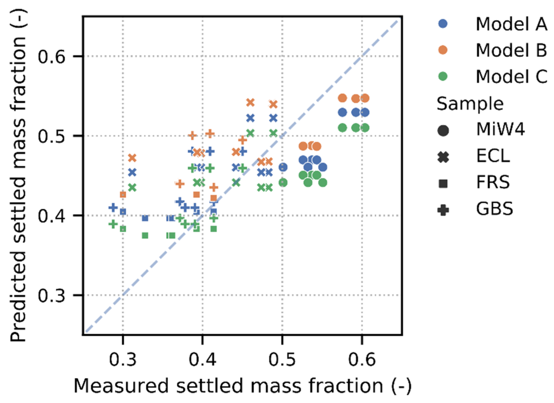
All settling models predicted the settled mass fraction with respect to t and wNaCl very well (Figure 5 and Figure S6). Model A was already able to predict the settled fraction, with a mean absolute error of 0.054 and a maximum residual error of 0.143. Thus, this simple model, with input variables PSD, ρs, t, and wNaCl, was sufficient to predict the outcome of the settling experiments. Model B considered additionally the withdrawn sample volume, which can extract nonsettled particles. However, it was not able to improve the prediction quality (mean absolute error of 0.059 and a maximum residual error of 0.161). Thus, the withdrawn sample volume seemed to be negligible. However, to meet quality assurance principles, the sample volume should be recorded. With consideration of the average particle shape of each RDS, Model C achieved a slight reduction of the mean absolute error to 0.050. The maximum residual error was 0.123. According to these results, the consideration of the nonsphericity of the particles does not considerably improve the prediction of RDS settling. If MiW4 is not considered, the mean absolute error of Models A and C are reduced to 0.050 and 0.037, respectively. The mean absolute error of Model B is increased to 0.064. The order of the predicted settled mass fractions by the models is Model C < Model A < Model B.
One unanticipated finding was that all models slightly underestimated the settled mass fraction of MiW4, while the settled mass of the nonartificial RDS was overestimated to a minor extent. As dynamic image analysis revealed that the PSDs of all samples, except for MiW4, differ from the Weibull PSD in the fine fraction, the deviation can be partly explained by the PSD. However, within the experiment duration of 4 min, it is mainly particles deq > 60 µm that settle. Another possible explanation can be that even though all samples showed comparable mass fraction weighted median φRiley, MiW4 showed a narrower φRiley distribution with respect to deq (Figure 1b and Figure S3). Consequently, MiW4 settles faster due to the smaller fraction of irregular-shaped particles, which exhibit lower settling velocities (Figure S7). Another source of bias was that the loss of particulate mass was considerably lower in the MiW4 experiments (1.8%) in contrast to the experiments with the real RDSs (3.6%). Thus, the overestimation of the settled fraction of the real RDSs can be partly explained by a mass loss during the experiments. Furthermore, the results are biased by the assumption of constant density with respect to particle size. The settled fractions of samples ECL and FRS, which mainly consisted of particles with deq >60 µm, showed lower ρs than the average ρs of the whole sample. Hence, the mass of the settled fraction was overestimated, although this is not valid for GBS. With respect to these uncertainties in the experiments and modeling, the used models showed an acceptable error. Nevertheless, it must be emphasized that the proposed models are designed to evaluate influencing factors in settling column experiments under varying boundary conditions (PSD, ρs, t, wNaCl, ϕ). Other approaches to model settling in full-scale SQIDs under dynamic conditions exist [21,22,56].
4. Conclusions
This study used preprocessed RDSs to reduce the effect of varying PSDs in order to assess effects caused by particle density, particle shape, temperature, and deicing salt concentration of the fluid.
Based on the experimental results, it was possible to validate and further develop the proposed method of Rommel and Helmreich [9], which is capable of modeling settling experiments with varying boundary conditions (PSD, ρs, t, wNaCl, ϕ). All analyzed RDSs featured comparable particle shapes, independent from their origin. Consideration of the particle shape did not significantly improve the modeling results. Based on these findings, particle shape was negligible to describe the settling of RDS. Future studies are needed to verify this based on more samples of various sites. Furthermore, very fine particles, significantly smaller than 60 µm, need to be studied as they potentially stay in suspensions for a long time and can be elutriated from SQIDs. This is of special importance due to the well-described high contaminant load in the fine particulate fraction.
The main limitation of the utilized settling experiments is that potentially occurring stratification in SQIDs cannot be reproduced. Thus, direct conclusions for SQIDs cannot be drawn. Future studies should assess the effect of stratification caused by temperature and salinity deviations using pilot or full-scale SQIDs and CFD modeling. Furthermore, road runoff underlies varying PM and hydraulic properties of intra- and inter-rain events. As RDS properties are site-specific, further investigations are necessary to predict site-specific PM properties.
Nevertheless, the gained knowledge on RDS properties can be used to evaluate future artificial RDSs for the assessment of SQIDs. In addition, the proposed model was able to deliver further insights into the relative contribution of the fluid and particle properties on the settling of RDS.
Supplementary Materials
The following are available online at https://www.mdpi.com/2073-4441/12/11/3126/s1. Figure S1: Bland–Altman plot for comparison of the two methods for the determination of the settled fraction (evaporation and filtration); the area between the dashed lines indicates the 95% confidence interval, n = 9; one outlier was removed. Figure S2: Particle size distribution of the preprocessed road-deposited sediments; fitted Weibull distribution for subsequent modeling of the sedimentation processes. Figure S3: 2D histogram of φRiley with respect to deq of all analyzed samples; color opacity indicates the density of counts; ECL n = 130,986, FRS n = 211,209, GBS n = 134,392, MiW4 n = 57,973. Figure S4: Mass fraction weighted histogram of the aspect ratios of the analyzed samples; ECL n = 130,986, FRS n = 211,209, GBS n = 134,392, MiW4 n = 57,973. Figure S5: Comparison of the experimental results of the settling experiments conducted by two different executers using the method described in this paper; n = 27. Figure S6: Settled mass fraction in the settling experiments; n = 3 for each experiment; the error bars indicate the standard deviation; experiment FRS, 21 °C, 0g/L was not conducted due to low sample quantity; marker shows the predicted settled mass fraction determined by Models A and C. Figure S7: Settling velocity determined with the equations proposed by Haider and Levenspiel (Model C) with respect to particle diameter and sphericity at 20 °C, ρs of MiW4, and wNaCl = 0. Supplementary Material A: model code. Supplementary Material B: modeling input data.
Author Contributions
Conceptualization, S.H.R., L.G., and A.W.; methodology, S.H.R. and L.G.; software, S.H.R.; validation, S.H.R.; investigation, S.H.R. and L.G.; resources, A.W. and B.H.; data curation, S.H.R. and L.G.; writing—original draft preparation, S.H.R.; writing—review and editing, S.H.R., L.G., A.W., and B.H.; visualization, S.H.R.; supervision, A.W. and B.H.; project administration, A.W. and B.H.; funding acquisition, A.W. and B.H. All authors have read and agreed to the published version of the manuscript.
Funding
This research received no external funding.
Acknowledgments
We thank Matthias Schwibinger of the Institute of Urban Water Management and Hydromechanics, Frankfurt University of Applied Science, and Sebastian Schott of the Chair of Urban Water Systems Engineering, Technical University of Munich, for their assistance in the experiments.
Conflicts of Interest
The authors declare no conflict of interest.
Nomenclature
| Symbol | Description |
| AR | Aspect ratio |
| CD | Drag coefficient |
| CFD | Computational fluid dynamics |
| d | Particle diameter |
| d* | Dimensionless particle diameter |
| Dc | Diameter of the smallest circumscribed circle |
| deq | Area equivalent circle diameter |
| Di | Diameter of the largest inscribed circle |
| g | Acceleration due to gravity |
| LOI | Loss on ignition |
| PM | Particulate matter |
| PSD | Particle size distribution |
| RDS | Road deposited sediment |
| SCM | Stormwater control measure |
| SQID | Stormwater quality improvement device |
| t | Temperature of the fluid |
| w | Terminal settling velocity |
| w* | Dimensionless settling velocity |
| wNaCl | Mass fraction of the NaCl in the fluid |
| ηf | Dynamic viscosity of fluid |
| νf | Kinematic viscosity of fluid |
| ρf | Fluid density |
| ρs | Particle density |
| ϕ | Particle sphericity |
| φRiley | Riley circularity |
References
- Stone, M.; Marsalek, J. Trace metal composition and speciation in street sediment: Sault Ste. Marie, Canada. Water Air Soil Pollut. 1996, 87, 149–169. [Google Scholar] [CrossRef]
- Sutherland, R.A.; Tolosa, C.A. Multi-element analysis of road-deposited sediment in an urban drainage basin, Honolulu, Hawaii. Environ. Pollut. 2000, 110, 483–495. [Google Scholar] [CrossRef]
- Sutherland, R.A.; Tack, F.M.G.; Ziegler, A.D. Road-deposited sediments in an urban environment: A first look at sequentially extracted element loads in grain size fractions. J. Hazard. Mater. 2012, 225–226, 54–62. [Google Scholar] [CrossRef] [PubMed]
- Loganathan, P.; Vigneswaran, S.; Kandasamy, J. Road-Deposited Sediment Pollutants: A Critical Review of their Characteristics, Source Apportionment, and Management. Crit. Rev. Environ. Sci. Technol. 2013, 43, 1315–1348. [Google Scholar] [CrossRef]
- Murakami, M.; Nakajima, F.; Furumai, H. Size- and density-distributions and sources of polycyclic aromatic hydrocarbons in urban road dust. Chemosphere 2005, 61, 783–791. [Google Scholar] [CrossRef] [PubMed]
- Zgheib, S.; Moilleron, R.; Saad, M.; Chebbo, G. Partition of pollution between dissolved and particulate phases: What about emerging substances in urban stormwater catchments? Water Res. 2011, 45, 913–925. [Google Scholar] [CrossRef] [PubMed]
- Dierkes, C.; Lucke, T.; Helmreich, B. General Technical Approvals for Decentralised Sustainable Urban Drainage Systems (SUDS)—The Current Situation in Germany. Sustainability 2015, 7, 3031–3051. [Google Scholar] [CrossRef] [Green Version]
- Goonetilleke, A.; Lampard, J.-L. Chapter 3—Stormwater Quality, Pollutant Sources, Processes, and Treatment Options. In Approaches to Water Sensitive Urban Design; Sharma, A.K., Gardner, T., Begbie, D., Eds.; Woodhead Publishing: Cambridge, UK, 2019; pp. 49–74. ISBN 978-0-12-812843-5. [Google Scholar]
- Rommel, S.H.; Helmreich, B. Influence of Temperature and De-Icing Salt on the Sedimentation of Particulate Matter in Traffic Area Runoff. Water 2018, 10, 1738. [Google Scholar] [CrossRef] [Green Version]
- Roseen, R.M.; Ballestero, T.P.; Houle, J.J.; Avellaneda, P.; Briggs, J.; Fowler, G.; Wildey, R. Seasonal Performance Variations for Storm-Water Management Systems in Cold Climate Conditions. J. Environ. Eng. 2009, 135, 128–137. [Google Scholar] [CrossRef]
- Semadeni-Davies, A. Winter performance of an urban stormwater pond in southern Sweden. Hydrol. Process. 2006, 20, 165–182. [Google Scholar] [CrossRef]
- Torres, A.; Bertrand-Krajewski, J.-L. Evaluation of uncertainties in settling velocities of particles in urban stormwater runoff. Water Sci. Technol. 2008, 57, 1389–1396. [Google Scholar] [CrossRef] [Green Version]
- Kang, J.; Li, Y.; Lau, S.; Kayhanian, M.; Stenstrom, M. Particle Destabilization in Highway Runoff to Optimize Pollutant Removal. J. Environ. Eng. 2007, 133, 426–434. [Google Scholar] [CrossRef]
- Gunawardana, C.; Egodawatta, P.; Goonetilleke, A. Role of particle size and composition in metal adsorption by solids deposited on urban road surfaces. Environ. Pollut. 2014, 184, 44–53. [Google Scholar] [CrossRef] [PubMed] [Green Version]
- Kayhanian, M.; McKenzie, E.R.; Leatherbarrow, J.E.; Young, T.M. Characteristics of road sediment fractionated particles captured from paved surfaces, surface run-off and detention basins. Sci. Total Environ. 2012, 439, 172–186. [Google Scholar] [CrossRef]
- McKenzie, E.; Wong, C.; Green, P.; Kayhanian, M.; Young, T. Size dependent elemental composition of road-associated particles. Sci. Total Environ. 2008, 398, 145–153. [Google Scholar] [CrossRef] [Green Version]
- Gelhardt, L.; Huber, M.; Welker, A. Development of a Laboratory Method for the Comparison of Settling Processes of Road-Deposited Sediments with Artificial Test Material. WaterAir Soil Pollut. 2017, 228, 467. [Google Scholar] [CrossRef]
- Li, Y.; Lau, S.-L.; Kayhanian, M.; Stenstrom, M.K. Particle size distribution in highway runoff. J. Environ. Eng. 2005, 131, 1267–1276. [Google Scholar] [CrossRef]
- Li, Y.; Lau, S.; Kayhanian, M.; Stenstrom, M. Dynamic Characteristics of Particle Size Distribution in Highway Runoff: Implications for Settling Tank Design. J. Environ. Eng. 2006, 132, 852–861. [Google Scholar] [CrossRef]
- Kayhanian, M.; Rasa, E.; Vichare, A.; Leatherbarrow, J. Utility of Suspended Solid Measurements for Storm-Water Runoff Treatment. J. Environ. Eng. 2008, 134, 712–721. [Google Scholar] [CrossRef]
- Li, Y.; Kang, J.-H.; Lau, S.-L.; Kayhanian, M.; Stenstrom, M.K. Optimization of settling tank design to remove particles and metals. J. Environ. Eng. 2008, 134, 885–894. [Google Scholar] [CrossRef] [Green Version]
- Spelman, D.; Sansalone, J.J. Is the Treatment Response of Manufactured BMPs to Urban Drainage PM Loads Portable? J. Environ. Eng. 2018, 144, 04018013. [Google Scholar] [CrossRef]
- Lin, H.; Ying, G.; Sansalone, J. Granulometry of Non-colloidal Particulate Matter Transported by Urban Runoff. Water Air Soil Pollut. 2009, 198, 269–284. [Google Scholar] [CrossRef]
- Laliberté, M.; Cooper, W.E. Model for calculating the density of aqueous electrolyte solutions. J. Chem. Eng. Data 2004, 49, 1141–1151. [Google Scholar] [CrossRef]
- Laliberté, M. Model for Calculating the Viscosity of Aqueous Solutions. J. Chem. Eng. Data 2007, 52, 321–335. [Google Scholar] [CrossRef]
- Hettler, E.N.; Gulliver, J.S.; Kayhanian, M. An elutriation device to measure particle settling velocity in urban runoff. Sci. Total Environ. 2011, 409, 5444–5453. [Google Scholar] [CrossRef] [PubMed]
- Aiguier, E.; Chebbo, G.; Bertrand-Krajewski, J.-L.; Hedgest, P.; Tyack, N. Methods for determining the settling velocity profiles of solids in storm sewage. Water Sci. Technol. 1996, 33, 117–125. [Google Scholar] [CrossRef]
- Michelbach, S.; Wöhrle, C. Settleable solids in a combined sewer system, settling characteristics, heavy metals, efficiency of storm water tanks. Water Sci. Technol. 1993, 27, 153–164. [Google Scholar] [CrossRef]
- Ying, G.; Sansalone, J. Gravitational Settling Velocity Regimes for Heterodisperse Urban Drainage Particulate Matter. J. Environ. Eng. 2011, 137, 15–27. [Google Scholar] [CrossRef]
- Blott, S.J.; Pye, K. Particle shape: A review and new methods of characterization and classification. Sedimentology 2008, 55, 31–63. [Google Scholar] [CrossRef]
- Breakey, D.E.S.; Vaezi, G.F.; Masliyah, J.H.; Sanders, R.S. Side-view-only determination of drag coefficient and settling velocity for non-spherical particles. Powder Technol. 2018, 339, 182–191. [Google Scholar] [CrossRef]
- Connolly, B.J.; Loth, E.; Smith, C.F. Shape and drag of irregular angular particles and test dust. Powder Technol. 2020, 363, 275–285. [Google Scholar] [CrossRef]
- Wang, Y.; Zhou, L.; Wu, Y.; Yang, Q. New simple correlation formula for the drag coefficient of calcareous sand particles of highly irregular shape. Powder Technol. 2018, 326, 379–392. [Google Scholar] [CrossRef]
- Bagheri, G.; Bonadonna, C. On the drag of freely falling non-spherical particles. Powder Technol. 2016, 301, 526–544. [Google Scholar] [CrossRef] [Green Version]
- DIBt. Teil 1: Anlagen zur dezentralen Behandlung des Abwassers von Kfz-Verkehrsflächen zur anschließenden Versickerung in Boden und Grundwasser; Zulassungsgrundsätze Niederschlagswasserbehandlungsanlagen; Deutsches Institut für Bautechnik: Berlin, Germany, 2017. [Google Scholar]
- Dierkes, C.; Welker, A.; Dierschke, M. Development of testing procedures for the certification of decentralized stormwater treatment facilities—Results of laboratory tests. NOVATECH 2013, 2013, 1–10. [Google Scholar]
- Riley, N.A. Projection sphericity. J. Sediment. Res. 1941, 11, 94–95. [Google Scholar]
- Bagheri, G.H.; Bonadonna, C.; Manzella, I.; Vonlanthen, P. On the characterization of size and shape of irregular particles. Powder Technol. 2015, 270, 141–153. [Google Scholar] [CrossRef]
- Huber, M.; Welker, A.; Drewes, J.E.; Helmreich, B. Auftausalze im Straßenwinterdienst-Aufkommen und Bedeutung für dezentrale Behandlungsanlagen von Verkehrsflächenabflüssen zur Versickerung. Abwasser 2015, 156, 1138–1152. [Google Scholar]
- Hilliges, R.; Endres, M.; Tiffert, A.; Brenner, E.; Marks, T. Characterization of road runoff with regard to seasonal variations, particle size distribution and the correlation of fine particles and pollutants. Water Sci. Technol. 2017, 75, 1169–1176. [Google Scholar] [CrossRef] [Green Version]
- American Public Health Association; American Water Works Association; Water Environment Federation (Eds.) Standard Methods for the Examination of Water and Wastewater; American Public Health Association: Washington, DC, USA, 2017; ISBN 978-0-87553-287-5. [Google Scholar]
- Virtanen, P.; Gommers, R.; Oliphant, T.E.; Haberland, M.; Reddy, T.; Cournapeau, D.; Burovski, E.; Peterson, P.; Weckesser, W.; Bright, J.; et al. SciPy 1.0: Fundamental algorithms for scientific computing in python. Nat. Methods 2020, 17, 261–272. [Google Scholar] [CrossRef] [Green Version]
- The Pandas Development Team. Pandas-Dev/Pandas: Pandas; Zenodo: Geneva, Switzerland, 2020. [Google Scholar]
- Hunter, J.D. Matplotlib: A 2D graphics environment. Comput. Sci. Eng. 2007, 9, 90–95. [Google Scholar] [CrossRef]
- Waskom, M.; Botvinnik, O.; Ostblom, J.; Gelbart, M.; Lukauskas, S.; Hobson, P.; Gemperline, D.C.; Augspurger, T.; Halchenko, Y.; Cole, J.B.; et al. Mwaskom/Seaborn: v0.10.1 (April 2020); Zenodo: Geneva, Switzerland, 2020. [Google Scholar]
- Lee, D.H.; Min, K.S.; Kang, J.-H. Performance evaluation and a sizing method for hydrodynamic separators treating urban stormwater runoff. Water Sci. Technol. 2014, 69, 2122–2131. [Google Scholar] [CrossRef]
- Selbig, W.R.; Fienen, M.N. Regression Modeling of Particle Size Distributions in Urban Storm Water: Advancements through Improved Sample Collection Methods. J. Environ. Eng. 2012, 138, 1186–1193. [Google Scholar] [CrossRef]
- Haider, A.; Levenspiel, O. Drag coefficient and terminal velocity of spherical and nonspherical particles. Powder Technol. 1989, 58, 63–70. [Google Scholar] [CrossRef]
- Cheng, N.-S. Comparison of formulas for drag coefficient and settling velocity of spherical particles. Powder Technol. 2009, 189, 395–398. [Google Scholar] [CrossRef]
- Chhabra, R.P.; Agarwal, L.; Sinha, N.K. Drag on non-spherical particles: An evaluation of available methods. Powder Technol. 1999, 101, 288–295. [Google Scholar] [CrossRef]
- Pedregosa, F.; Varoquaux, G.; Gramfort, A.; Michel, V.; Thirion, B.; Grisel, O.; Blondel, M.; Prettenhofer, P.; Weiss, R.; Dubourg, V.; et al. Scikit-learn: Machine learning in Python. J. Mach. Learn. Res. 2011, 12, 2825–2830. [Google Scholar]
- Seabold, S.; Perktold, J. statsmodels: Econometric and statistical modeling with python. In Proceedings of the 9th python in science conference, Austin, TX, USA, 28 June–3 July 2010. [Google Scholar]
- Kayhanian, M.; Givens, B. Processing and analysis of roadway runoff micro (<20 μm) particles. J. Environ. Monit. 2011, 13, 2720–2727. [Google Scholar]
- Kreider, M.L.; Panko, J.M.; McAtee, B.L.; Sweet, L.I.; Finley, B.L. Physical and chemical characterization of tire-related particles: Comparison of particles generated using different methodologies. Sci. Total Environ. 2010, 408, 652–659. [Google Scholar] [CrossRef]
- Chebbo, G.; Gromaire, M.-C. VICAS—An Operating Protocol to Measure the Distributions of Suspended Solid Settling Velocities within Urban Drainage Samples. J. Environ. Eng. 2009, 135, 768–775. [Google Scholar] [CrossRef]
- Abrishamchi, A.; Massoudieh, A.M. Kayhanian Probabilistic modeling of detention basins for highway stormwater runoff pollutant removal efficiency. Urban Water J. 2010, 7, 357–366. [Google Scholar] [CrossRef]
Figure 1.
(a) Particle size distribution (PSD) of the analyzed samples and the fitted Weibull PSD used for the subsequent modeling, particle count: Eckenheimer Landstraße (ECL) n = 515,545; Frauensteinstraße (FRS) n = 593,302; Glauburgstraße (GBS) n = 540,036; MiW4 n = 501,254. (b) Mass fraction weighted histogram of φRiley of the analyzed samples, particle count: ECL n = 130,986; FRS n = 211,209; GBS n = 134,392; MiW4 n = 57,973.

Figure 2.
Microscopic images of some road-deposited sediment (RDS) particles of the sample ECL, captured using dynamic image analysis. The particle shape of the other samples was comparable. The images are not scaled.
Figure 2.
Microscopic images of some road-deposited sediment (RDS) particles of the sample ECL, captured using dynamic image analysis. The particle shape of the other samples was comparable. The images are not scaled.
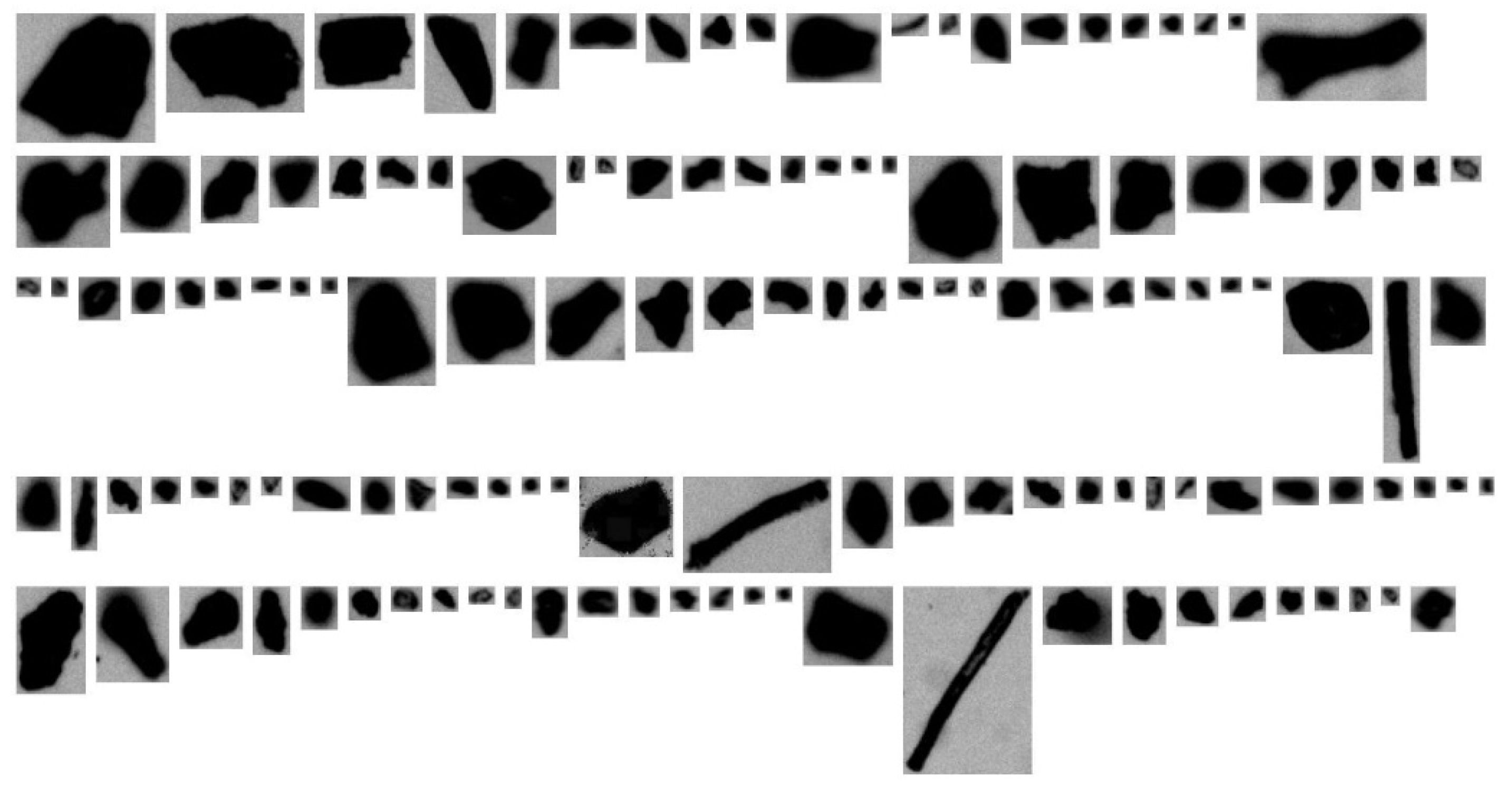
Figure 3.
Settled mass fraction in the settling experiments with varying temperatures (21 and 10 °C) and NaCl concentrations (0 and 20 g/L); n = 3 for each experiment. The error bars indicate the standard deviation; the asterisks (*) indicate statistically significant differences between two experiments (p < 0.05). Experiment FRS 21 °C 0 g/L NaCl was not conducted due to low sample quantity.
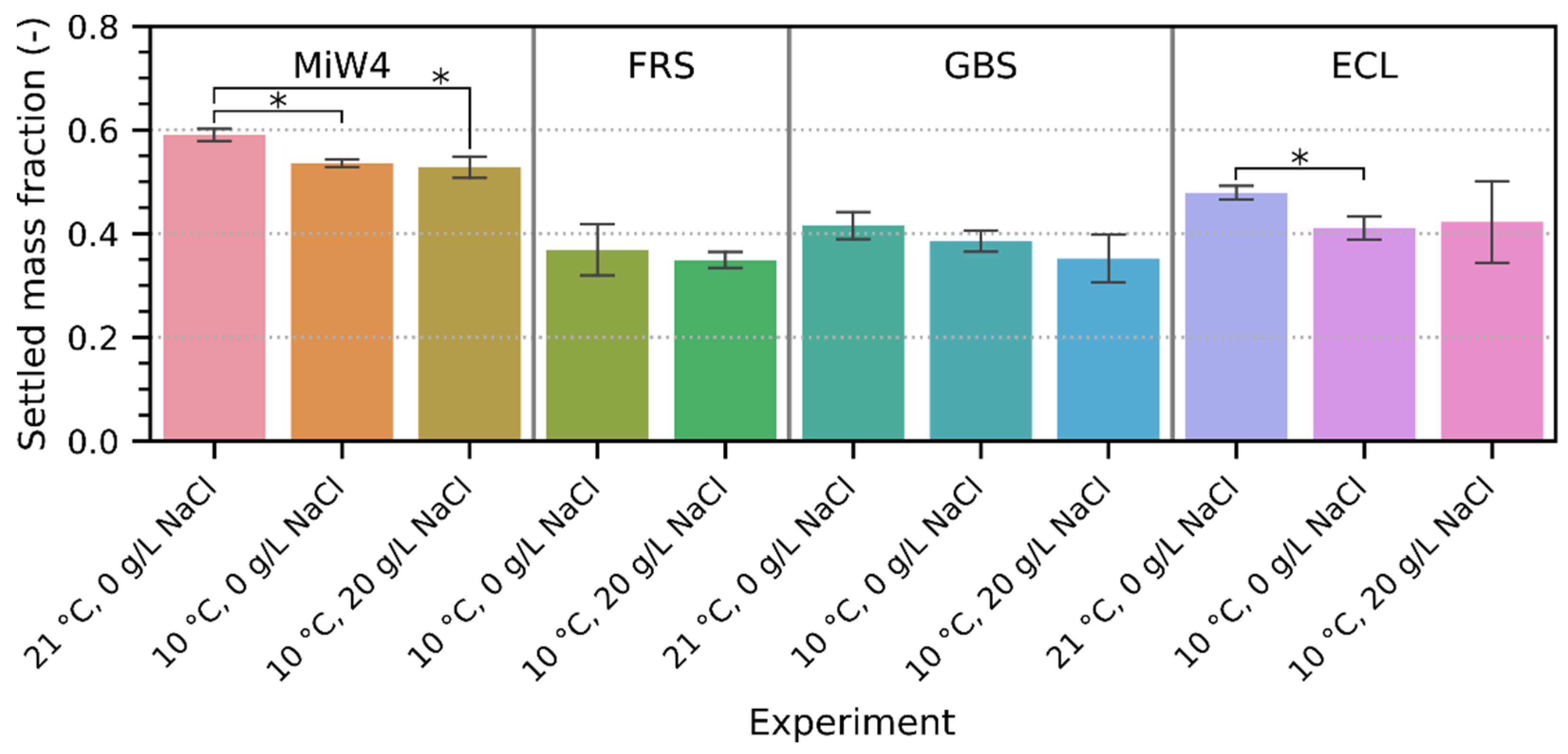
Figure 4.
Settled mass fraction in the settling experiments with respect to ρs, t, and LOI; n = 33.

Figure 5.
Comparison between measured and predicted settled mass fraction by Models A, B, and C of all samples (MiW4, ECL, FRS, and GBS); n = 33.
Figure 5.
Comparison between measured and predicted settled mass fraction by Models A, B, and C of all samples (MiW4, ECL, FRS, and GBS); n = 33.

Table 1.
Characteristics of sampling site and studied materials (< 250 µm), LOI (loss on ignition), and ρs (particle density) were calculated after fractionation and recomposition, as described below.
Table 1.
Characteristics of sampling site and studied materials (< 250 µm), LOI (loss on ignition), and ρs (particle density) were calculated after fractionation and recomposition, as described below.
| Sample | Location | Coordinate | Sampling Date | AADT (Vehicles/d) | LOI (%) | ρs (g cm−3) |
|---|---|---|---|---|---|---|
| MiW4 a | – | – | – | – | <0.1 | 2.65 |
| ECL | Eckenheimer Landstraße | 50°07′57.2″ N 8°41′03.5″ E | 18 July 2017 | 8500 | 7.6 | 2.60 |
| GBS b | Glauburgstraße | 50°07′38.6″ N 8°41′28.0″ E | 6 April 2017 b 12 April 2017 b 21 April 2017 b | 9600 | 17.5 | 2.32 |
| FRS | Frauensteinstraße | 50°07′51.1″ N 8°40′47.7″ E | 17 October 2017 | 150 | 22.2 | 2.25 |
a Standard mineral material; b The sample GBS was a composite sample of three samples due to low quantity.
Table 2.
Particle size distribution of the road-deposited sediments used within this study.
| Size Fraction | Weight | Cumulative Weight |
|---|---|---|
| (µm) | (%) | (%) |
| 200–250 | 4 | 100 |
| 160–200 | 6 | 96 |
| 125–160 | 12 | 90 |
| 100–125 | 8 | 78 |
| 63–100 | 21 | 70 |
| 40–63 | 15 | 49 |
| <40 | 34 | 34 |
Table 3.
Particle density (ρs) of the fractionated samples ECL, FRS, and GBS.
| Size Fraction (µm) | ρs (g cm−3) | ||
|---|---|---|---|
| ECL | FRS | GBS | |
| 200–250 | 2.56 | 2.25 | 2.41 |
| 160–200 | 2.54 | 2.17 | 2.37 |
| 125–160 | 2.57 | 2.14 | 2.31 |
| 100–125 | 2.55 | 2.18 | 2.32 |
| 63–100 | 2.61 | 2.20 | 2.30 |
| 40–63 | 2.65 | 2.31 | 2.31 |
| <40 | 2.61 | 2.34 | 2.32 |
Publisher’s Note: MDPI stays neutral with regard to jurisdictional claims in published maps and institutional affiliations. |
© 2020 by the authors. Licensee MDPI, Basel, Switzerland. This article is an open access article distributed under the terms and conditions of the Creative Commons Attribution (CC BY) license (http://creativecommons.org/licenses/by/4.0/).
Share and Cite
MDPI and ACS Style
Rommel, S.H.; Gelhardt, L.; Welker, A.; Helmreich, B. Settling of Road-Deposited Sediment: Influence of Particle Density, Shape, Low Temperatures, and Deicing Salt. Water 2020, 12, 3126. https://doi.org/10.3390/w12113126
AMA Style
Rommel SH, Gelhardt L, Welker A, Helmreich B. Settling of Road-Deposited Sediment: Influence of Particle Density, Shape, Low Temperatures, and Deicing Salt. Water. 2020; 12(11):3126. https://doi.org/10.3390/w12113126
Chicago/Turabian StyleRommel, Steffen H., Laura Gelhardt, Antje Welker, and Brigitte Helmreich. 2020. "Settling of Road-Deposited Sediment: Influence of Particle Density, Shape, Low Temperatures, and Deicing Salt" Water 12, no. 11: 3126. https://doi.org/10.3390/w12113126
Note that from the first issue of 2016, this journal uses article numbers instead of page numbers. See further details here.