Hydrological Early Warning System Based on a Deep Learning Runoff Model Coupled with a Meteorological Forecast


1
Departamento de Ingeniería Civil, Universidad de Chile, Santiago 8370448, Chile
2
Departamento de Ingeniería Mecánica, Universidad de Chile, Santiago 8370448, Chile
3
Modelación Ambiental SpA, Santiago 7500015, Chile
*
Author to whom correspondence should be addressed.
Water 2019, 11(9), 1808; https://doi.org/10.3390/w11091808
Submission received: 1 August 2019
/
Revised: 20 August 2019
/
Accepted: 26 August 2019
/
Published: 30 August 2019
(This article belongs to the Section Hydrology)
Abstract
:The intensification of the hydrological cycle because of global warming raises concerns about future floods and their impact on large cities where exposure to these events has also increased. The development of adequate adaptation solutions such as early warning systems is crucial. Here, we used deep learning (DL) for weather-runoff forecasting in región Metropolitana of Chile, a large urban area in a valley at the foot of the Andes Mountains, with more than 7 million inhabitants. The final goal of this research is to develop an effective forecasting system to provide timely information and support in real-time decision making. For this purpose, we implemented a coupled model of a near-future global meteorological forecast with a short-range runoff forecasting system. Starting from a traditional hydrological conceptual model, we defined the hydro-meteorological and geomorphological variables that were used in the data-driven weather-runoff forecast models. The meteorological variables were obtained through statistical scaling of the Global Forecast System (GFS), thus enabling near-future prediction, and two data-driven approaches were implemented for predicting the entire hourly flow time-series in the near future (3 days), a simple Artificial Neural Networks (ANN) and a Deep Learning (DL) approach based on Long-Short Term Memory (LSTM) cells. We show that the coupling between meteorological forecasts and data-driven weather-runoff forecast models are able to satisfy two basic requirements that any early warning system should have: The forecast should be given in advance, and it should be accurate and reliable. In this context, DL significantly improves runoff forecast when compared with a traditional data-driven approach such as ANN, being accurate in predicting time-evolution of output variables, with an error of 5% for DL, measured in terms of the root mean square error (RMSE) for predicting the peak flow, compared to 15.5% error for ANN, which is adequate to warn communities at risk and initiate disaster response operations.
1. Introduction
In the last decade, a series of unprecedented extreme hydrological events have occurred, some of which have been attributed to climate change [1]. In fact, global projections indicate a positive correlation between global warming and the risk of extreme rainfall and floods [2]. This intensification of the hydrological cycle raises growing concerns about future floods and their impact on large cities where exposure has also increased [3]. Adequate adaptation solutions are required to increase resilience and reduce vulnerability of large urban centers. In this sense, the development of early warning technologies is crucial because it allows the localization of resources, the warning of communities at risk, and the initiation of disaster response operations [4].
The great difficulty in developing forecasting tools and early warning systems in the field of hydrology is that the physical mechanisms involved in the runoff processes are non-linear and extremely difficult to model, so that runoff forecasting models have a high uncertainty [5]. Furthermore, an early warning system should be able to give accurate warning for extreme events, but also should be able to give accurate forecasts for small flows to avoid false positive warnings that eventually reduce the reliability of the system [6]. Given that the early warning systems give more importance to the simplicity and robustness of the forecasting model rather than an accurate description of the various internal sub-processes, it is certainly worth considering hybrid models that combine physical-based models with data-driven approaches for improving real-time runoff forecasts [7,8,9,10]. Another difficulty in predicting hydrological extremes is that to get ahead of an extreme event requires the implementation of weather forecasting models coupled to hydrological models. The development of this type of coupled systems has not had much development, mainly because the global climate models (GCMs) have had very coarse spatial resolution; so that, they did not have the ability to forecast extreme events with the degree of precision that is required in the scale of hydrological systems [11]. However, today there are high resolution global weather forecast models, which in conjunction with novel downscaling techniques, allows the development of model-generated weather input data for hydrological forecasting models [12,13].
The development of Machine Learning (ML) and Deep Learning (DL) techniques, on the other hand, have recently boosted the use of data-driven approaches as a complement to traditional methods for the prediction and forecasting of hydrological variables, in which Artificial Neural Networks (ANN) are the most commonly used technique for this task [8,14,15,16,17]. Furthermore, an improvement of this approach has been achieved with neuro-fuzzy systems, which combines the human-like reasoning of a fuzzy system with the learning capability of neural networks [18]. This hybrid scheme has shown good results for rainfall-runoff modeling when comparing with the ANN approach alone [19,20]. Nevertheless, approaches such as ANN are not exactly adequate for the analysis of sequential data. To address this challenge, various methods have been developed to keep a certain memory of the previous state of the system, thus allowing the prediction to use not only the present information but also the previous state. One of the most successful techniques is the Long-Short Term Memory (LSTM) cells, which are based on Recurrent Neural Networks (RNN). This type of model has been widely used to achieve state-of-the-art results on sequence modeling tasks such as handwriting recognition [21,22], speech recognition [23], time series prediction [24,25,26] and robot control [27], among others. In this sense, the new learning algorithms and architectures that are currently being developed for neural networks allow the acceleration of the development of hydrological forecasting and early warning tools [28].
There are not many applications of DL in the field of hydrology [29], among which DL is included for daily flows in a seasonal time-frame only based on flow observations [30], and rainfall-runoff models that predict hourly flow only based on observed precipitation [25]. Furthermore, a comparison between a physical-based model with four recurrent neural networks is presented in [31], showing that data-driven models perform better. For the case of hydrological extremes, LSTM networks have been used in rainfall-runoff models to predict daily flow in several basins in the USA [32], showing an improvement in predictions with LSTM networks compared to a traditional hydrological model; however, other studies argued that these results could have been improved by using the specific hydro-meteorological and geomorphological variables of each basin [33]. Furthermore, hydrological applications of DL have been usually developed based on real time field observations of rainfall and flow (see [33] and references therein), thus limiting the runoff forecast to the timescale defined by the catchment concentration time (e.g., [6]). One alternative to increase the runoff forecast timescale is to link the runoff forecasts with near-future global meteorological forecasts that are capable of predicting rainfall, air temperature, and other input variables in a longer timescale. To our understanding, this link has not been previously explored.
In this article, we used deep learning (DL) for weather-runoff forecasting in región Metropolitana of Chile, a large urban area in a valley at the foot of the Andes Mountains, with more than seven million inhabitants. The final goal of this research is to develop an effective forecasting system to provide timely information and support in real-time decision making, as an adaptation to hydrological extremes in a warming climate. For this purpose, we implemented a coupled model of near-future global meteorological forecast with short-range runoff forecasting systems based on DL. Starting from a traditional hydrological model, we defined the conceptual model and the hydro-meteorological variables that were used in the training of the data-driven models. The meteorological variables were obtained through statistical scaling of the Global Forecast System (GFS). Two data-driven models were implemented for runoff forecasts, a simple Artificial Neural Networks (ANN) and a Deep Learning (DL) approach based on Long-Short Term Memory (LSTM) cells. With these two approaches, we predicted at once the entire hourly flow time-series for 1 day in the past and 3 days in the future with no need for the entire record of past flow measurements, just the flow at t = 0. This was a constraint required to be considered because of it is not possible to rely on always having a continuum time series of real-time observations, so we decided to minimize the real-time information needed for forecasting the flow. Finally, the same data was used in both data-driven techniques, in which the data were separated into training, validating and testing data sets, and the model skills were compared through different metrics.
As far as we know, the novelties of this contribution that have not been previously published are: (i) We present an approach based on a DL model that is coupled a near-future global meteorological forecast with a short-range runoff forecasting system. (ii) We use the complete set of hydro-meteorological and geomorphological variables of a complex hydrological model for training the data-driven models. (iii) Our approach is capable of predicting an output time-series with a finer temporal resolution than the input time-series. This temporal downscaling allows us to precisely locate the time at which the peak flow will occur. (iv) Finally, our approach predicts at once the entire hourly flow time-series for 1 day in the past and 3 days in the future with no need of the entire record of past flow measurements, just the flow at t = 0.
This paper is organized as follows: In the next section we describe the two algorithms used in this article (ANN and DL), present the study site composed of nine flow stations, and detail the methodology that couples meteorological forecast with data-driven weather-runoff forecast models. Two alternatives for the data-driven weather-forecast model are described that aim to predict the detailed hourly flow time-series for the following three days—ANN and DL approaches. In the results section we present the results in terms of the model’s performance in predicting the flow conditions for the following 3 days, in which we compare the performance of the two data-driven approaches. Finally, in the discussion and conclusion sections, we highlight and summarize the key features and limitations of the proposed methodology.
2. Materials and Methods
2.1. Data-Driven Techniques
We used Artificial Neural Networks (ANN) [34] and a Deep Learning (DL) approach based on Long-Short Term Memory (LSTM) cells [35], which are described next.
2.1.1. Artificial Neural Networks
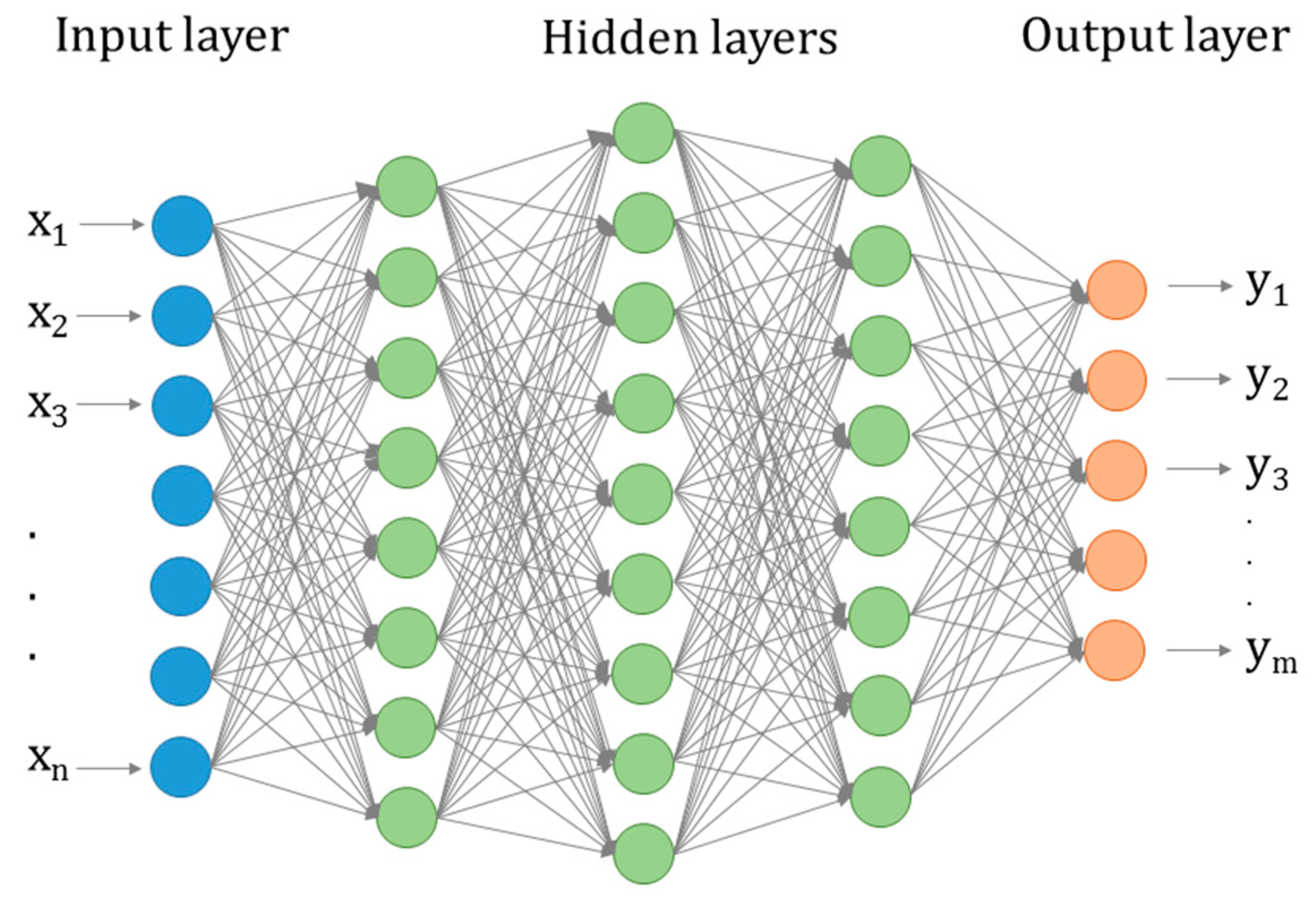
As illustrated in Figure 1, an ANN, also known as a multilayer perceptron, consists of an arrangement of input neurons known as the input layer, an arrangement of output neurons known as the output layer and a number of hidden layers. Each neuron receives a weighted sum from the neurons in the previous layer and gives an input to every neuron of the next layer. The activation of each neuron is governed by a function known as the transfer function.
These networks, are also known as feedforward neural networks because the information is transmitted in only one direction, forward from the input layer to the output layer. Therefore, there are no backward connections between layers (cycles or loops).
As an example, the outputs of a three-layer ANN are given by
where and are the input and output vectors, and are the interconnection weights, represents the bias (or threshold) terms and is the transfer function, usually a sigmoid function. The training problem consists of finding the weights and biases that will minimize the mean square error between the network prediction and the output targets.
2.1.2. Deep Learning Based on LSTM Neural Networks
Recurrent Neural Networks (RNNs) are one of the most powerful type of Neural Networks, capable of processing sequences of arbitrary input patterns [36]. RNNs, however, suffer from the vanishing gradient problem, which makes it difficult to perform backpropagation efficiently during training, causing great computational effort. To overcome this, alternative structures have been proposed, such as Gated Recurrent Units and the LSTM cells.
Figure 2 illustrates the flow of a time series through an unrolled LSTM layer. In this diagram, corresponds to a vector of input features, hi denote the output vectors and ci denote the cell states, all of them evaluated at the i-th time step.
The classical LSTM block structure shown in Figure 2b consists of different processes called gates [37]. These gates compute the desired output from a new input data at a time , along with elements obtained from the previous time step .
Equations (2)–(7) describe the processes in an LSTM block. Equations (2)–(4) represent the input, output and forget gate. These gates compute a linear combination of the new input data with the output of the previous time step , which are evaluated using a sigmoid activation function. On the other hand, gate generates candidates that will become part of the new cell state. Equation (6) corresponds to the cell state , which represents a memory capsule containing information of all previous states. Finally, the output is computed by the element wise multiplication of the output gate with the activation of the cell state (Equation (7)). It should be noted that gates , , and represent independent neural networks, which possess their own weights and biases.
2.2. Hydrological Description of the Study Area
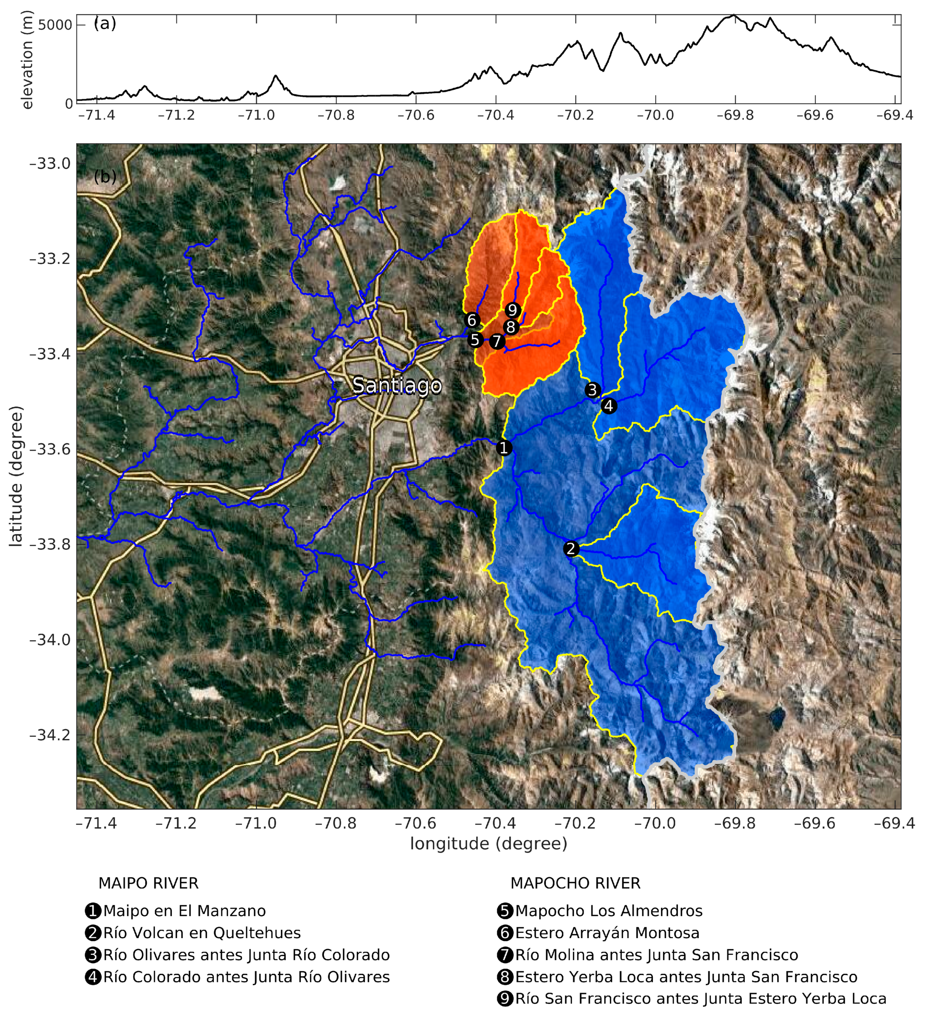
Región Metropolitana (33.5° S, 70.8° W, 500 m a.s.l.) is located in central Chile, in the Maipo river watershed, at the foot of the Andes Mountain that have an average height of 3000 m above sea level (m a.s.l.) and maximum height of 6500 m a.s.l. Two rivers coming from the Andes Mountains pass across region Metropolitana: Maipo river in the south, and Mapocho river in the north (Figure 3). These rivers come from the high mountains range, above 3500 m a.s.l, in an area covered by discontinuous permafrost, snow and glaciers. In this area, glaciers occupy near 8% of the total surface (Table 1), and it was estimated that nearly 10% of the rest of the detrital surface is occupied by debris-covered glaciers [38].
During the colder months in the Austral winter, disturbances of the polar front, which usually affect the southern part of Chile, move northwards and generate sporadic eruptions of precipitation systems in central Chile. Consequently, rainfall is recorded occasionally and they show great irregularity, with an annual average of 350 mm in the valley and increasing with height, and snow accumulation above 1500 m a.s.l in the winter months [39]. Nevertheless, convective rainfall in high altitude can also be expected during summer time under warm conditions with elevated 0 °C isotherm. On the other hand, the austral summer dominance of the subtropical anticyclone results in hot and dry summers, thus resulting in a semi-arid climate [39].
As a consequence, the Mapocho and Maipo rivers have a complex hydrological regime, which can be classified as a pluvio-nival regime during the autumn–winter seasons and a nivo-glacial regime during the spring–summer seasons. In this context, air temperature and humidity are as important as precipitation to determine the river flows, as they define the contributing area and the rate at which snow and glaciers melt.
2.3. Coupled Model of a Meteorological Forecast with a Short-Range Runoff Forecast
We implemented a coupled model of a near-future global meteorological forecast with short-range runoff forecasting systems that we call data-driven weather-runoff forecast models, which were designed to forecast the flow in the nine different flow stations shown in Figure 3, for which we used as an input data the Global Forecast System (GFS) provided by the National Centers for Environmental Prediction (NCEP) for the following 3 days. The NCEP model was used because it has had a meteorological analysis since March 2004, with a meteorological forecast that has been run under the same mesh grid and with the same parametrizations, thus allowing the use of historical meteorological forecasts for training, validating and testing data-driven runoff forecast models, as explained below.
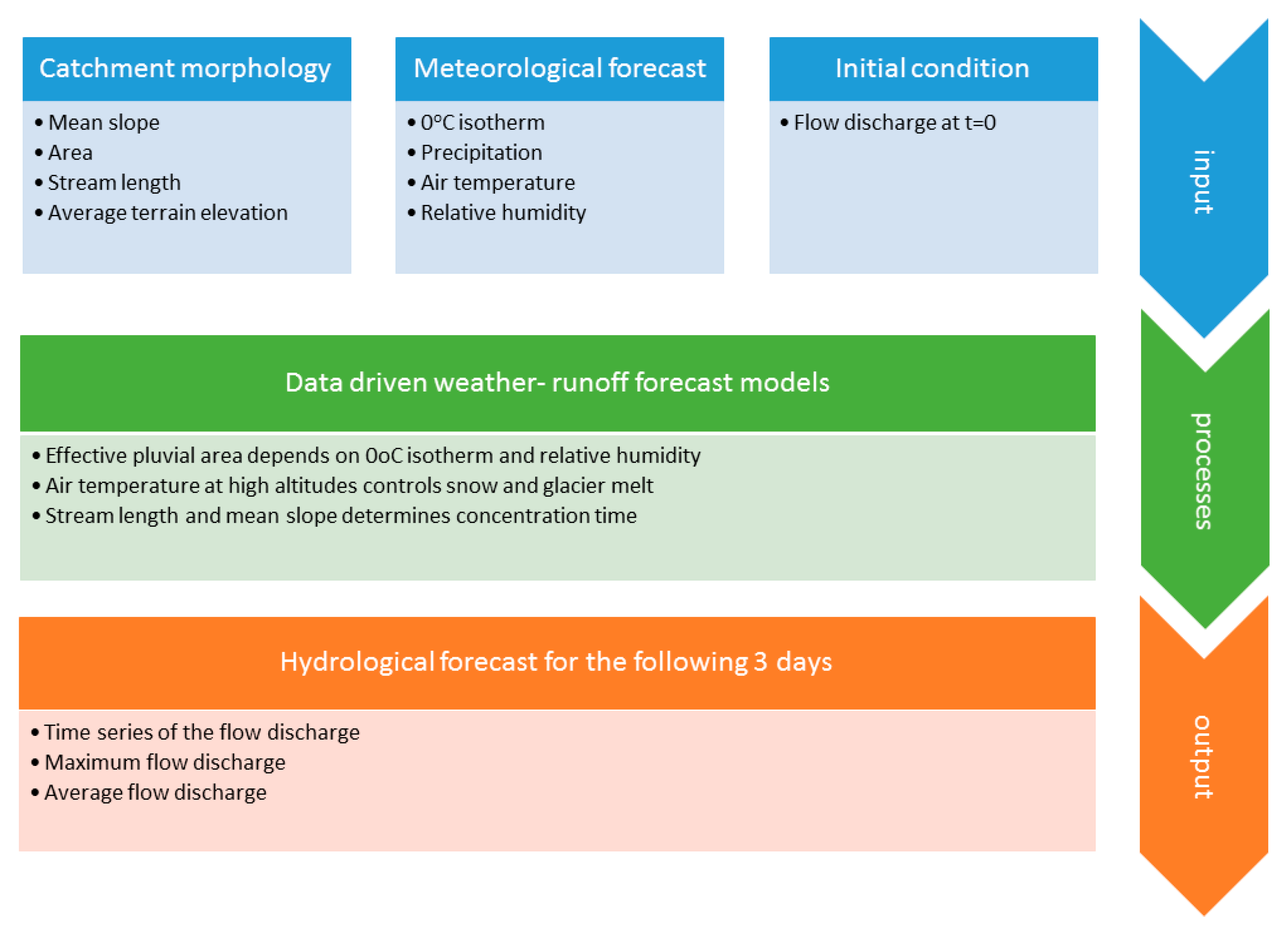
The flowchart of the weather-runoff forecast models is shown in Figure 4, in which three different groups of input data were identified to train the data-driven weather-runoff forecast models: watershed morphology, meteorology, and initial condition. The data-driven runoff model was designed to predict entire hourly flow time-series for the following 3 days, based on two different data-driven approaches: ANN and DL models. Below is described the input data and the structure of the different runoff models.
2.3.1. Input Data
In Section 2.2, the hydrological description of the study area has shown that the Mapocho and Maipo rivers regime can be classified as a pluvio-nival regime during the autumn–winter seasons and a nivo-glacial regime during the spring–summer seasons. As a consequence, the variables for the weather-runoff model includes the standard variables in a rainfall-runoff model (precipitation, catchment area, stream length, slope), as well as air temperature and humidity as they define the contributing area and the rate at which snow and glaciers melt. Considering this, three different group of input information were used (Figure 4):
- Watershed geomorphology: The geomorphological characteristics were calculated from NASA Shuttle Radar Topography Mission (SRTM) version 3.0 global 1 arc second. For this aim, the watershed associated to each one of the flow stations was defined, and the information was summarized in one single table that list as a function of the elevation, the following information: Watershed area (km2); length of the mainstream (km); maximum, minimum and average elevation of the watershed; and the average slope. This table is read at each time to create time series of the geomorphological information as a function of the 0 °C isotherm elevation that splits the watershed into solid and liquid precipitation areas. Besides the watershed area, the time-series of the length of the mainstream, and the average slope and maximum elevation of the watershed were used as inputs of the data-driven weather-runoff models, as they are associated with the computation of the concentration time of the watershed [40]. The average elevation of the watershed was used to vertically interpolate the precipitation time-series from the GFS-NCEP meteorological model.
- Meteorological forecast: The weather forecast was obtained from a statistical scaling of gridded data of the GFS provided by NCEP, from which we obtained precipitation and air relative humidity at the average elevation of the watershed below the 0 °C isotherm, and air temperature at 2 m above the terrain in 3500 m a.s.l, and this reference terrain elevation was the same for all of the nine catchments. This last variable was chosen based on preliminary trial and error tests that showed that it gave better results in the representation of diurnal flow pulses during snow melt. We tested for other constant reference elevations (2000 and 4000 m a.s.l), and the results were not sensitive to this value. Furthermore, without good results, we also tested as reference temperature, the temperature at the average elevation of the catchment below the 0 °C isotherm that varies in time. We used the forecast datasets with a horizontal resolution of 0.5 × 0.5 degree, available from 2004 to present, and with a horizontal resolution of 0.25 × 0.25 degree, available from 2007 to present. Vertical scaling of the GFS information was made by linearly interpolating the meteorological variables as a function of the terrain elevation, using the GFS grid points located in a 0.5 degree of radius, regardless of the horizontal resolution of the GFS model, following the vertical scaling methodology described in [41]. Furthermore, each forecast starts with the weather forecast and is updated every 6 h, at 0:00, 6:00, 12:00 and 18:00 h UTC-time.
- Initial condition: The present flow conditions of all nine flow stations were obtained from real-time hour measurements of the General Direction of Water of the Chilean government; so that, the observed flow was used as an initial condition (t = 0).
In summary, together with the flow observed at t = 0, weather-runoff forecast models receive as input the time-series of seven variables that describes temporal changes (1 day in the past and 3 days in the future) of the watershed morphology and meteorological conditions. These variables are: (i) Watershed area below the 0 °C isotherm; (ii) mainstream length below the 0 °C isotherm; (iii) average slope of the watershed below the 0 °C isotherm; (iv) elevation of the 0 °C isotherm; (v) precipitation rate and (vi) air relatively humidity, both vertically interpolated to the average elevation of the watershed; and (vii) air temperature at 3500 m a.s.l.
2.3.2. Data-Driven Weather-Runoff Forecast Models
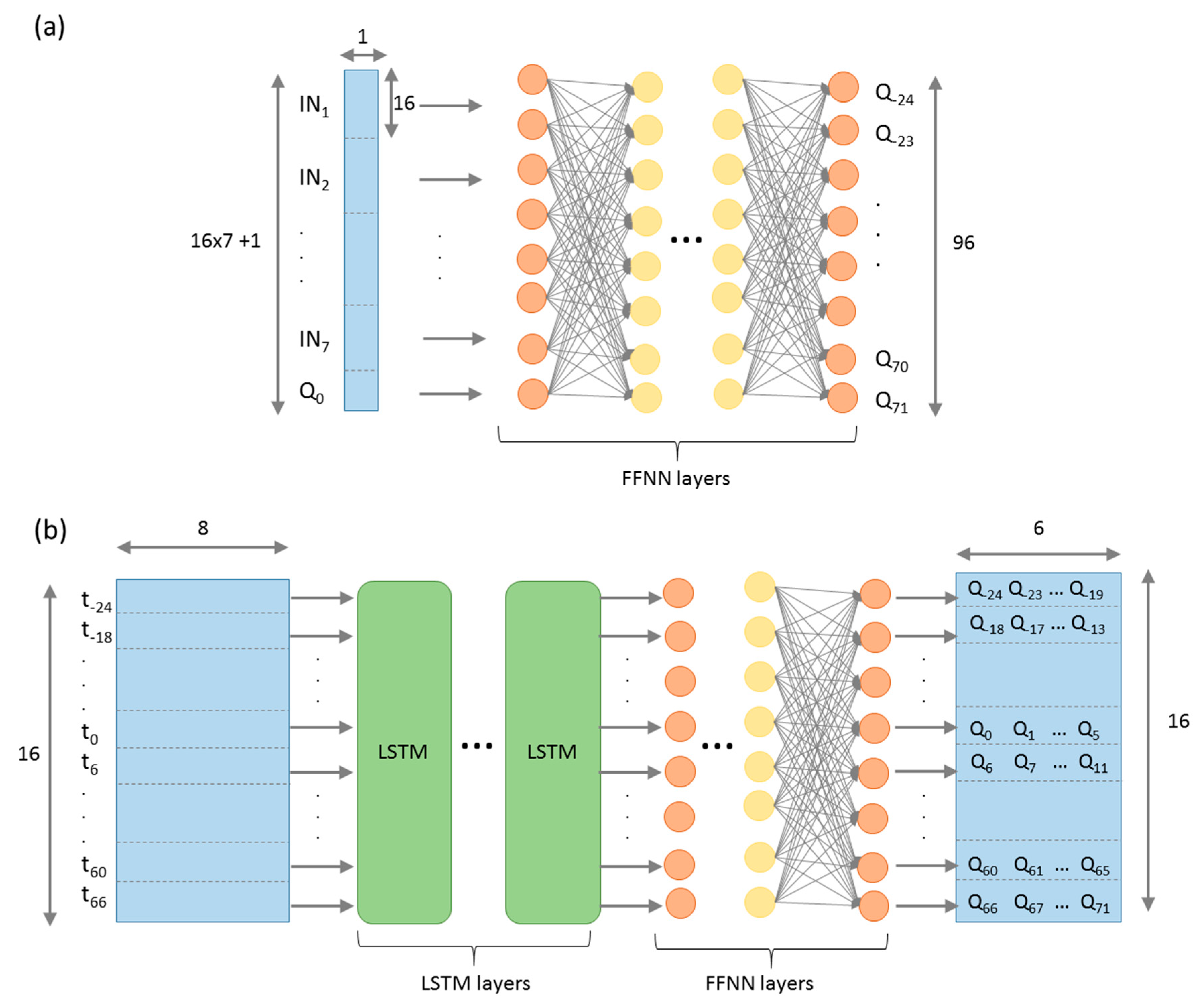
Two data-driven approaches were used for weather-runoff forecast models—the ANN and DL techniques—both aiming in predicting the entire hourly time-series of the flow rate for the next three days. Both forecasts used the observed flow in t = 0 plus the GFS weather information of the previous 24 h (4 observations at t = −24, −18, −12 and −6 h per each one of the input variables) and the following 3 days (12 observations at t = 0, 6, …, 66 h per each one of the input variables). We used Matlab© (version R2018b, www.matworks.com, USA) for the computation, in which the ANN model consists of a sequence of fully connected layers (FFNN), whereas the DL model combines LSTM layers followed by a sequence of FFNN layers (see Figure 5). The transfer functions in the FFNN layers, the number of FFNN and LSTM layers, and the number of hidden neurons in the LSTM and FFNN layers were determined by looking at the minimum root mean square error of the validation data set.
These forecast models aim to predict the flow time-series every hour based on the GFS weather data and the observed flow at t = 0. For doing this, the ANN model receives one vector of 113 inputs, corresponding to 112 GFS weather data (16 × 7) plus the observed flow at t = 0 (Figure 5a). The output is the predicted flow at t = −24, −23, …, +71, +72 h (96 outputs). The DL model, on the other hand, receives as input one 16 rows times 8 columns matrix, in which each row is associated with each one of the GFS times (t = −24, −18, …, +60, +66 h), whereas the columns contain the 7 input variables and the observed flow at t = 0, which is repeated on each row. The output is a 16 rows times 6 column matrix (Figure 5b), in which the first column contains the flow at times t = −24, −18, …, +60, +66 h, the second column the flow at t = −23, −17, …, +61, +67 h, and so on until the last column contains the flows at t = −19, −13, …, +65, +71 h. It is important to notice that the DL model was not used in the standard recursive way, in which the past time-series dependent variable (flow in this case) is recursively used as input for predicting the flows for the following time-steps. The proposed forecast model predicts at once the entire flow time-series for 1 day in the past and 3 days in the future with no need of the past flow. This constraint was required because the continuum real-time observations of the flow are not reliable, thus being necessary to only estimate the flow at t = 0 in case of failure of the real-time flow monitoring system. This is one of the novelties of this manuscript.
Finally, for both forecasts, the input and output variables were normalized by subtracting the mean value and dividing it by the standard deviation, and the entire data set obtained for each flow station was randomly subdivided into three subsets: 70% of the data set for training the weights of the net, 10% for validating (hyperparameter tuning), and 20% for testing (model evaluation). The testing subset is used for evaluating the metrics of the model skills. Table 2 summarizes the hydrological features (maximum flow, mean flow, minimum flow and percentile 90% and 99%) of each subset, for each one of the nine flow stations, showing that for each flow station, no significant differences in the hydrological characteristics as a function of the subset. This is an important aspect since previous research has shown that the decomposition into train, validation and test subsets has consequences on the final outcome of the data-driven model [20].
2.4. Evaluation Metrics for Model Skills
Six indexes were used to evaluate the performance of the trained models: the root mean square error (RMSE), the Nash–Sutcliffe efficiency index (NSE), the normalized RMSE by the average flow, Pearson correlation coefficient , the error of time to peak discharge and the error of peak discharge.
The root means square error, RMSE, is defined as
where and denotes the observed and predicted value, N the total number of observations used for computing RMSE. The RMSE has units of flow (m3/s) and quantifies the standard error in the prediction.
The NSE (Nash–Sutcliffe efficiency index) is defined as
where denotes the average observations. NSE is a dimensionless index that quantifies the magnitude of the RMSE with respect to the standard variation of the observed flows. NSE is equal to 1 for the perfect fit and it can take values smaller than 0 if the RMSE is larger than the standard deviation of the observations.
The normalized RMSE () is the RMSE divided by the average observed flow, and it quantifies the magnitude of the error with respect to the observed flow:
The correlation coefficient takes values between −1 and 1, being equal to 1 if there is a perfect correlation between observed and predicted flows, if there is a perfect inverse correlation, and is equal to 0 if there is no correlation between observed and predicted flows.
The error to maximum flow () was introduced by [25], and in the context of this article it quantify the relative error in predicting the maximum flow for the following three days. It is defined as
where denotes the measured maximum flow for the next three days, and the predicted maximum flow.
Finally, the error of time to maximum flow () was also introduced by [25], and it is the absolute difference in hours between the time at which the maximum flow is observed ( versus the time at which the maximum flow is simulated. (. It is defined as
The last two indexes are used to evaluate the performance of the early warning system.
2.5. Structure of the Data-Driven Weather-Runoff Forecasts Models
The structure of the ANN and DL weather-forecast models is defined by the transfer functions, the number of hidden layers and the number of hidden neurons, whose values were determined by minimizing the of the validation subset of Maipo en el Manzano, and the same structure was used for all of the flow stations.
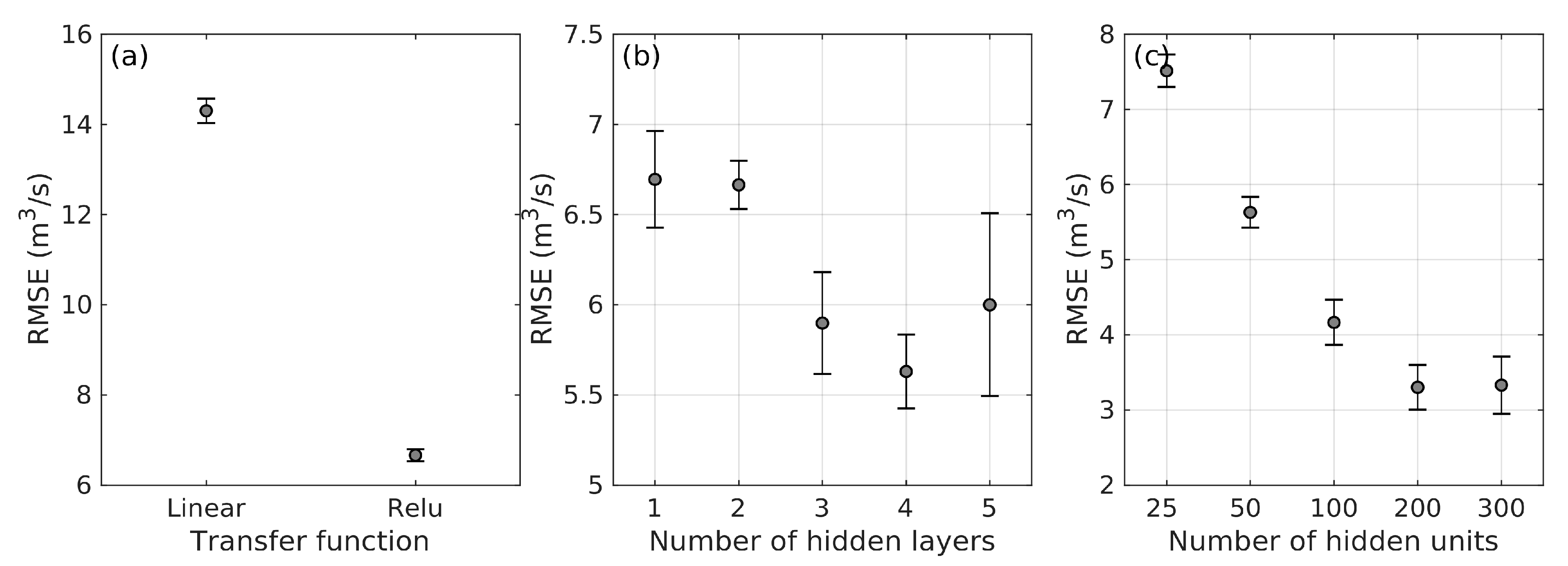
Table 3 lists the functions and parameters to be defined in the ANN model along with the range of values investigated. The number of layers and the number of hidden neurons were initially set equal to two and fifty, respectively. Then, the model was evaluated with two different transfer functions in the hidden layers: Linear and a rectified linear (Relu). The transfer function of the output layer was set to linear, which is recommended for regression problems. Each case was trained and evaluated ten times to characterize their variability. The results are presented in Figure 6a, the mean value is illustrated with a grey circle and the standard deviation by error bars. The best results are obtained with a Relu transfer function in the hidden layers. Then, the performance was evaluated with one to five hidden layers; each case was trained and evaluated ten times. The results presented in Figure 6b indicate that the best results are obtained with four hidden layers. Lastly, Figure 6c shows the performance with different number of neurons in the hidden layers, which is optimum for 300 neurons. Therefore, the final architecture that will be used hereinafter for the ANN model is four hidden layers with 300 neurons each and for Relu transfer functions, the output layer has 96 neurons and a linear transfer function.
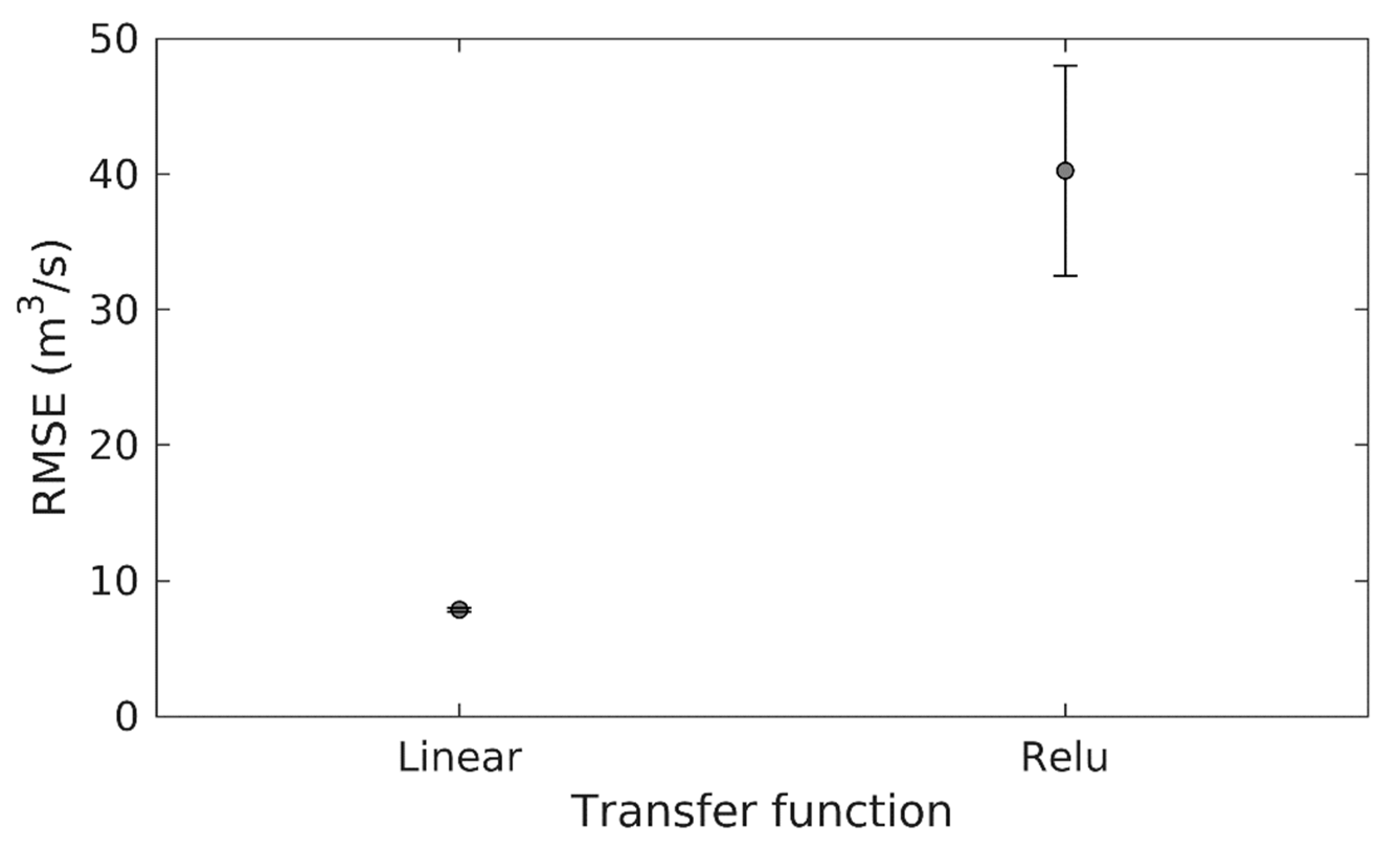
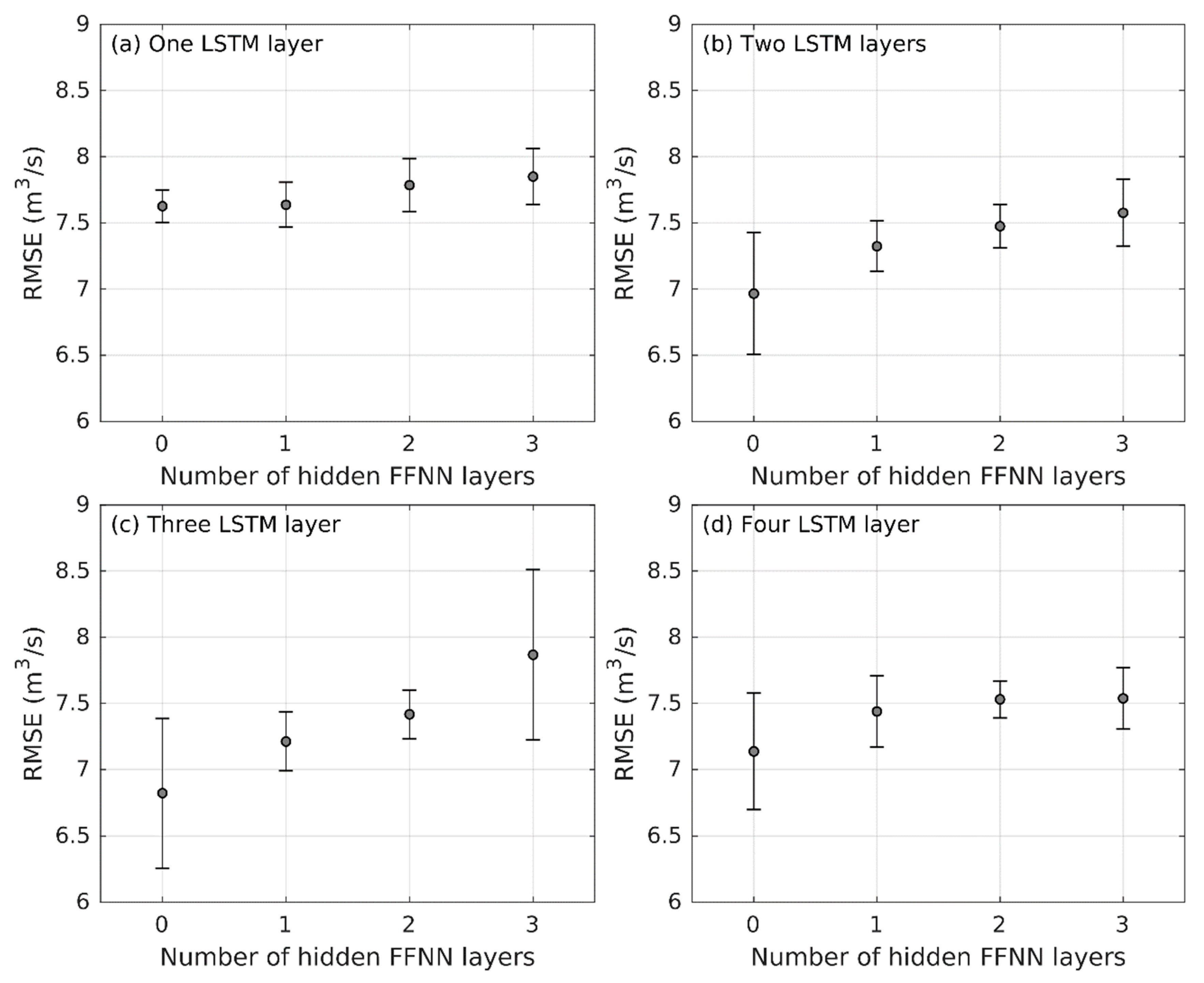
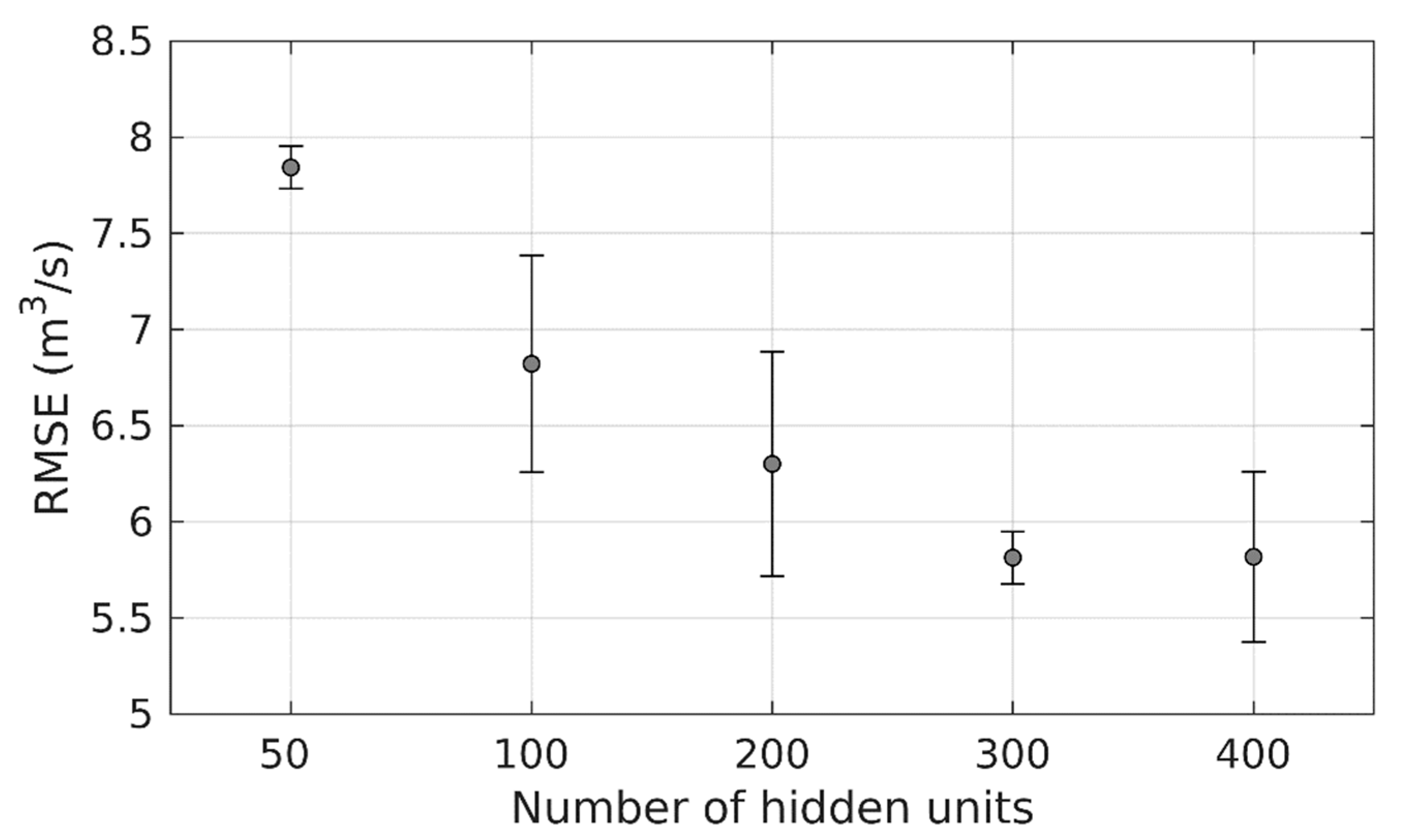
Furthermore, Table 4 lists the parameters and functions to be defined in the DL model along with the range of values investigated. The procedure to select the best parameters was the same for the ANN model. First, the number of neurons in the LSTM and FFNN hidden layers were set equal to one hundred and the number of LSTM and FFNN hidden layers to one and two, respectively. The transfer function of the FFNN output layer was set to linear and then the performance of the two transfer functions in the hidden FFNN layers was evaluated. Once the transfer functions were selected, the model was evaluated with different combinations for the number of LSTM and hidden FFNN layers. Finally, the model was evaluated for different number of hidden units. Each combination was trained and evaluated ten times with the validation subset of Maipo en el Manzano. The results of the sensitivity analysis are presented in Figure 7, Figure 8 and Figure 9. Therefore, the final architecture for the detailed forecast model is three LSTM layers with 300 neurons each and one output FFNN layer with a linear transfer function. This means that there are only two FFNN layers: The input and the output layers. This architecture will be used hereinafter for all nine flow stations.
3. Results
3.1. Performance of ANN versus DL Weather-Runoff Forecast Models
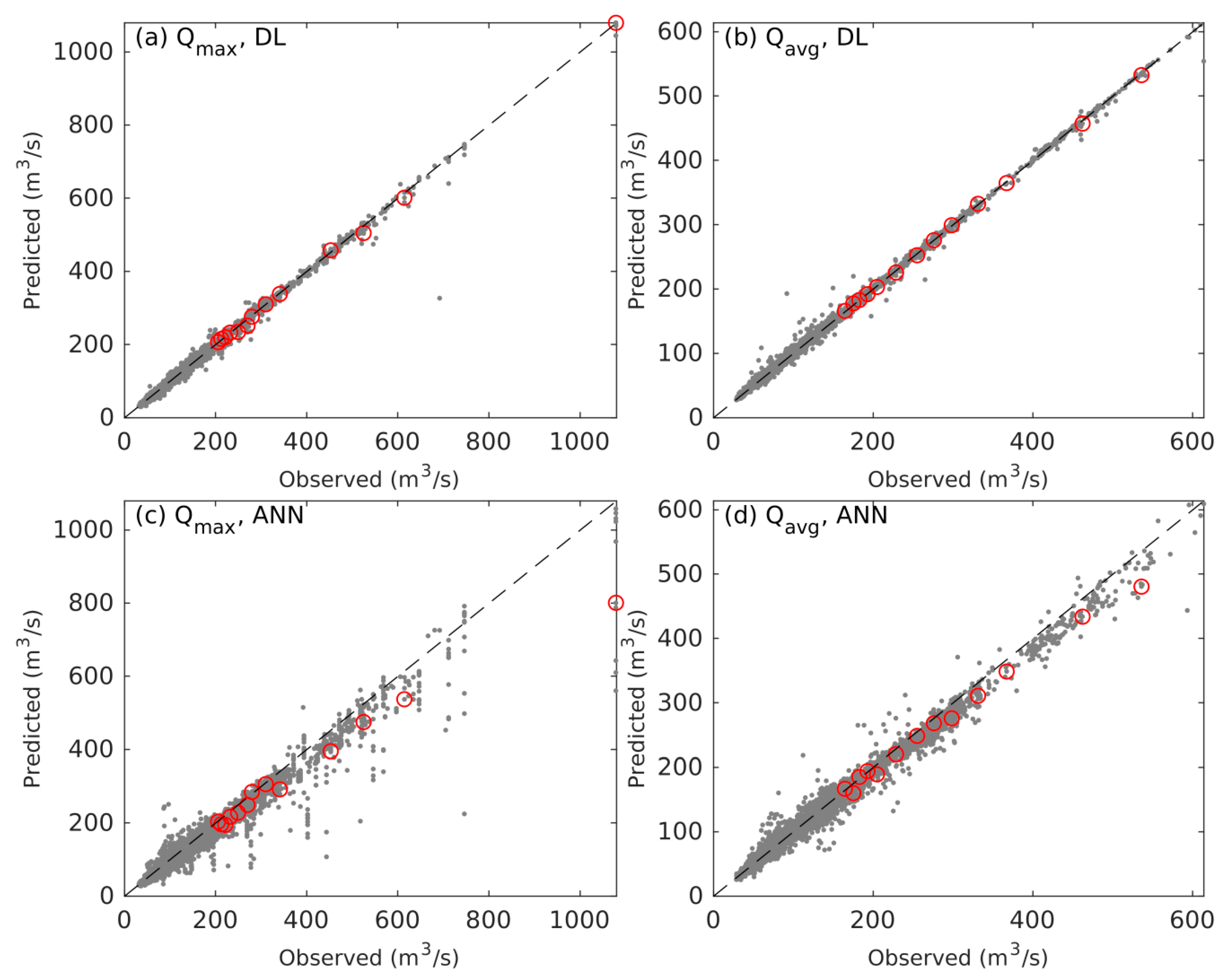
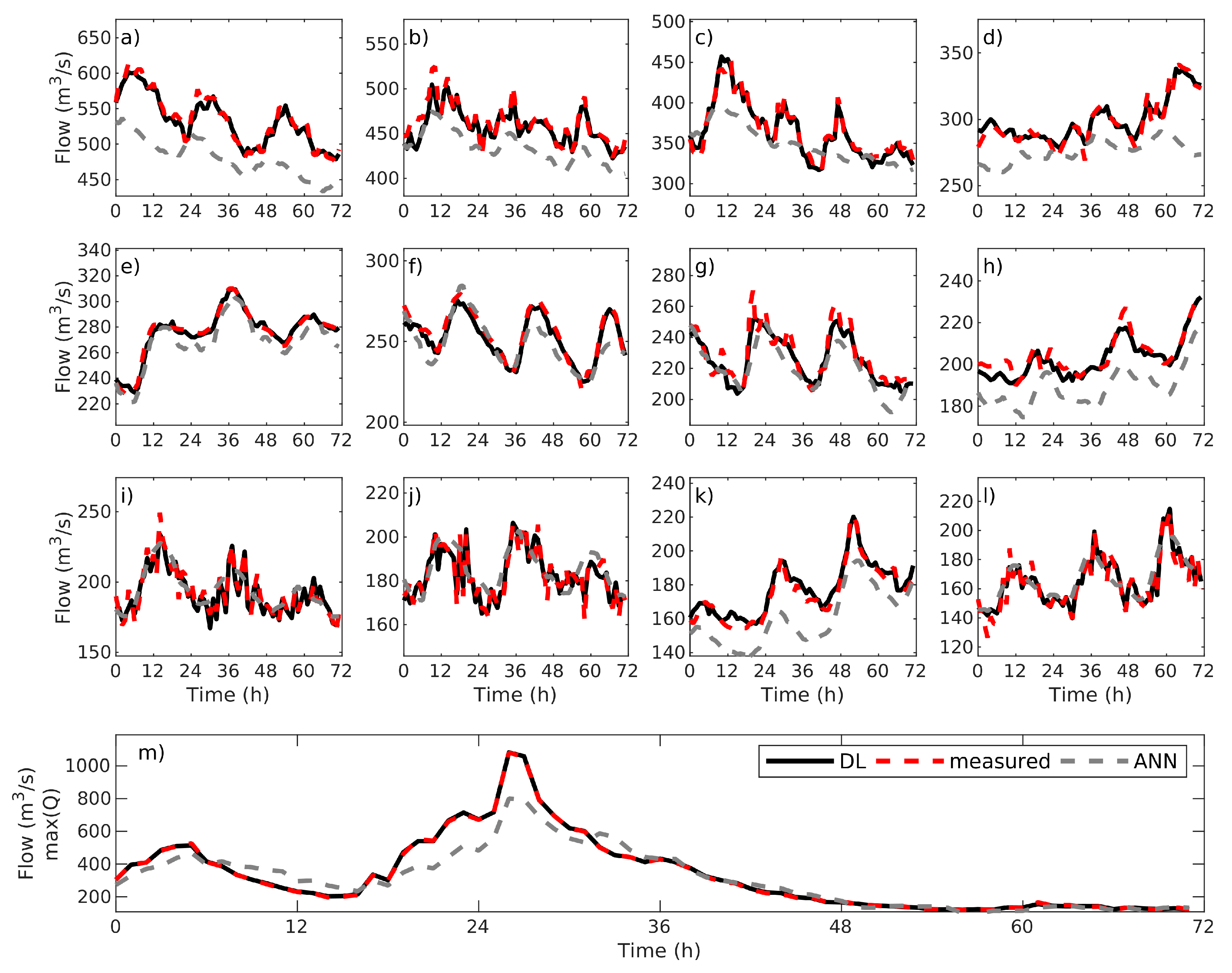
To evaluate the differences between the ANN and DL weather-runoff models, Figure 10 shows the direct comparison between observed and predicted maximum and average flow for the DL model ((a) and (b)) and the ANN model ((c) and (d)); using the test subset (the goodness of the fit is indicated in Table 5). The same figure for the rest of flow stations showed, in general, good agreement between predicted and observed maximum and average flows for both the DL and the ANN models, however, the performance of the DL weather-runoff model was better than the ANN model (see Figures S1–S8 in Supporting Information and Table 5). The normalized for the DL model were 5.9% and 4.3% for and , respectively; and were very close to 1, and the was 7.0 m3/s and 4.3 m3/s for and , respectively (see Table 5). With respect to performance in predicting the entire time-series of the flow for the following 3 days, Figure 11 shows the comparison between the observed and predicted flow for different cases identified with open circles in Figure 10. These examples were chosen based on the cumulative frequency of the average observed flow, using percentiles of 99.9%, 99.6%, 99%, 98%, 97%, 96%, 95%, 94%, 93%, 92%, 91% and 90%, for panels (a) to (l), respectively. Finally, Figure 11 compares predicted and observed flow time-series for the maximum flow event. Similar figures for the rest of the flow stations are found in the Supporting Information.
The results show that the ANN model makes an acceptable prediction of the average flow, but has difficulties in recognizing temporal changes. This is reflected in greater errors in the predicted maximum flow, with a tendency to underestimate it. This is explained by the fact that ANN do not have a temporal “memory”, and therefore are not good at predicting temporal changes. The DL model, which incorporates LSTM cells, has a much better prediction performance for the time-flow series as well as for the maximum and average flow, demonstrating that the temporal capacity of LSTM-based algorithms allows a prediction of temporal changes.
3.2. Performance of the Early Warning System
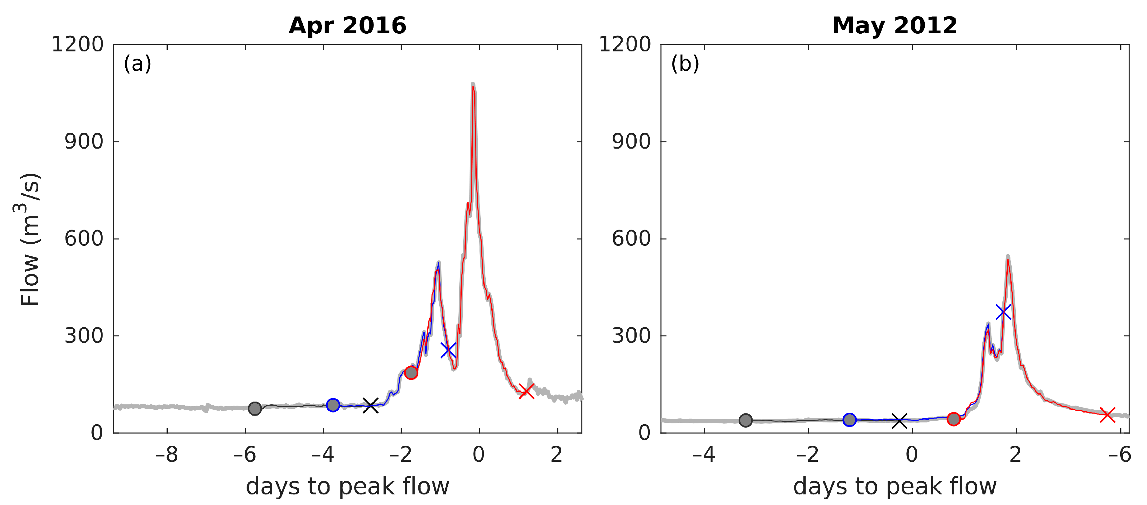
In order to verify the early warning advantage of the DL weather-runoff model, two extreme events were analyzed in detail. These events correspond to floods that occurred in April of 2016 (with a peak flow of 1078.6 m3/s, Figure 12a), and in May of 2012 (with a maximum flow of 546.1 m3/s, Figure 12b). For each event, the DL weather-runoff forecast model was run several times, starting at different days before the time at which the maximum flow was observed. As an example, Figure 12 shows three of these runs: One that starts 6 days before the peak flow and ends before the flow start to rise (black line that starts with the circle and ends with the black x); the second (blue simulation) that starts 4 days the peak flow, at the beginning of the storm, and ends before the peak flow was observed; and the third simulation starting on 2 days before the peak flow, in the middle of the storm, and ending after the peak flow has passed. Similarly, Table 6 shows the errors of time to peak ETp (Equation (13)), and peak discharge, EQp (Equation (12)), calculated for each one of the different simulations.
In terms of the early warning system, the blue simulation of April 2016 would have predicted at the beginning of the storm an important increase in the flow of Maipo River, while the red simulation would have predicted the magnitude and timing of the peak flow with two days in advance, as well as the flood duration. A similar situation is observed for the May 2012 event. In terms of the errors EQp and ETp (Table 6), the relative error in predicting the maximum flow tends to be smaller for larger maximum flows, and it takes positive values; so that, in this case, the model predicts maximum flows slightly smaller than the measurements. With respect to the error in the time to maximum flow, it is equal to 0 most of the time.
4. Discussion
In this article, we detailed a methodology that couples a process-based meteorological model that forecasts atmospheric conditions in the near future, with data-driven weather-runoff forecast models, which use these meteorological inputs for predicting hourly flow time-series in the near future. We implemented this methodology in región Metropolitana of Chile, for which two data-driven techniques were used for the weather-runoff forecast models—a simple ANN approach and a DL approach based on LSTM cells.
The data-driven weather-runoff models were designed based on the following three central ideas: (i) The near future flow (3 days) in the studied flow stations responds to both the precipitation rate of the storm, but also to changes in the watershed area or rate of snow melt (see Figure 11f). Consequently, a rainfall-runoff scheme (e.g., [25]) is not enough for predicting near-future flow, which justifies the weather-runoff concept that also uses air temperature and relatively humidity and the 0 °C isotherm for predicting the near-future flow. Both, air temperature and relatively humidity were important variables that improved the performance of the weather-runoff model in the preliminary exercises. Particularly, air temperature at 3500 m a.s.l. can be associated with snow melt rate, whereas air humidity at the 0 °C isotherm controls the limit between liquid and solid precipitation [42]. (ii) Real-time flow observations are in general available, but it is not possible to rely on the availability of a continuous measured time-series for forecasting the near-future flow, especially during large storms. As a consequence, the weather-runoff forecast model is predominantly based on the (very reliable) GFS-NCEP model, although the flow at is (always) needed as input. In case of not having flow observation for , this flow can be estimated using simple cross correlations with the other flow stations. (iii) Early warning systems should be able to give accurate warning for extreme events, but should also be able to give accurate forecasts for small flows to avoid false positive warnings that eventually reduce the reliability of the system [6,43]. In this context, both data-driven approaches used the entire set of flow observations for training, validating and testing the forecast models, without paying specific attention to high flow events which are the important ones in early warning systems. For example, the range of predicted flows in the Maipo en el Manzano station varies between 25 to 1100 m3/s.
With respect to the performance of data-driven weather-runoff forecast models, it is possible to argue that both approaches are accurate for predicting and ; however, flow prediction based on the DL approach is far more accurate than the flow prediction based on ANN approach, as shown in Table 5. This was pointed out by [25] with a rainfall-runoff model, and it is verified in this new approach with a weather-runoff model. The DL approach has an excellent performance, with values of RMSE 5%, compared to RMSE 15.5% for ANN approach for the prediction of the peak flow in station 1 (Table 5). These results are explained in the fact that, approaches such as ANN are not exactly adequate for the analysis of sequential data, such as the flow time series. To address the forecast of sequential data, is required to keep a certain memory of the previous state of the system, thus allowing the prediction using not only the present information but also the previous state. Since ANN do not have a temporal memory, they have difficulties in recognising temporal changes. This is reflected in greater error when predicting flow floods and therefore tend to underestimate the flow, as shown in Figure 11. In this context, one of the most successful techniques based on Recurrent Neural Networks (RNN) is the DL approach based on LSTM cells [24,25,26]. Although we use only one value of the flow as initial condition, the previous state for DL approach is obtaining through the seven sequences of the meteorological and geomorphological inputs of the previous days, which is used in the DL approach for generating the output sequential data.
Furthermore, another important feature of the proposed architecture of the DL weather-runoff forecast (Figure 5b) is that it is capable of predicting an output time-series with a finer temporal resolution (1 h) than for the input time-series (6 h), thus enabling the use of DL as a temporal downscaling technique. This allows to precisely locating the time at which the peak flow will occur, which gives the system an early warning advantage, as shown in Figure 12 and Table 6. The DL weather-runoff model is capable of capturing the peak flow, the time at which it will occur and the flow duration. All of this information would be available from three days in advance, which is very useful for allocating resources and warning the communities at risk.
Finally, it is important to notice that the methodology that was implemented for the nine flow stations in Maipo and Mapocho rivers, can, in principle, be scaled to the entire set of flow stations with real-time measurement in Chile (approximately 450 flow stations). The coupling between the GFS-NCEP model forecast and the DL weather-runoff forecast model may not vary; however, input variables to DL weather-runoff forecast model should be different in flow stations located in the desert of northern Chile (latitude: −22° S) to the flow stations located in the austral part of southern Chile (latitude: −45° S). For example, presumably, the air temperature associated to glacier melt should not be a relevant input data in northern Chile where there are no glaciers.
5. Conclusions
The intensification of the hydrological cycle because of the global warming raises growing concerns about future floods and their impact on large cities where exposure has also increased, such as the región Metropolitana of central Chile. Adequate water adaptation solutions as early warning systems are crucial. Given that the early warning systems give more importance to the simplicity and robustness of the forecasting model rather than an accurate description of the various internal sub-processes, it is certainly worth considering data-driven approaches for improving real-time runoff forecasts.
In this article, we implemented a coupled model of a near-future global meteorological forecast with short-range runoff forecasting systems based on DL, showing that DL is a valuable technique that allows the acceleration of the development of hydrological forecasting and early warning tools. The coupling between meteorological forecasts and the DL weather-runoff forecast model, on the other hand, are able to satisfy two basic requirements that any early warning system should have: The forecast should be given in advance in a time-frame larger than catchment concentration time, and should be accurate and reliable. In this context, meteorological forecasts are accurate and reliable in predicting near-future meteorological conditions, which feed the DL weather-runoff forecast, thus enabling a reliable flow forecast in advance.
Furthermore, DL significantly improves runoff forecasts when compared with a simple ANN approach, being accurate in predicting the time-evolution of output variables, with an error for predicting the peak flow of RMSE 5% compared to RMSE 15.5% for the ANN approach, which is adequate to warn communities at risk and initiate disaster response operations. Another interesting aspect of this approach is that it is capable of predicting an output time-series with a finer temporal resolution than the input time-series. This temporal downscaling allows us to precisely locate the time at which the peak flow will occur. Finally, the real-time implementation of these DL models can be found in the open access webpage www.AlertaHidrica.com.
Supplementary Materials
The following are available online at https://www.mdpi.com/2073-4441/11/9/1808/s1, Figures S1–S8 are to Figure 11 of the manuscript, but for stations 2–9. Figures S9–S16 are equivalent to Figure 12 of the manuscript, for stations 2–9. Figure S1: Station 2. (a) Comparison between observed and predicted for flow station 1 and the DL model. (b) Same as (a) for the average flow . (c) and (d) same as (a) and (b) for the ANN model. Red open circles define examples plotted in Figure S9. Figure S2: Station 3. (a) Comparison between observed and predicted for flow station 1 and the DL model. (b) Same as (a) for the average flow . (c) and (d) same as (a) and (b) for the ANN model. Red open circles define examples plotted in Figure S10. Figure S3: Station 4. (a) Comparison between observed and predicted for flow station 1 and the DL model. (b) Same as (a) for the average flow . (c) and (d) same as (a) and (b) for the ANN model. Red open circles define examples plotted in Figure S11. Figure S4: Station 5. (a) Comparison between observed and predicted for flow station 1 and the DL model. (b) Same as (a) for the average flow . (c) and (d) same as (a) and (b) for the ANN model. Red open circles define examples plotted in Figure S12. Figure S5: Station 6. (a) Comparison between observed and predicted for flow station 1 and the DL model. (b) Same as (a) for the average flow . (c) and (d) same as (a) and (b) for the ANN model. Red open circles define examples plotted in Figure S13. Figure S1: Station 7. (a) Comparison between observed and predicted for flow station 1 and the DL model. (b) Same as (a) for the average flow . (c) and (d) same as (a) and (b) for the ANN model. Red open circles define examples plotted in Figure S14. Figure S7: Station 8. (a) Comparison between observed and predicted for flow station 1 and the DL model. (b) Same as (a) for the average flow . (c) and (d) same as (a) and (b) for the ANN model. Red open circles define examples plotted in Figure S15. Figure S2: Station 9. (a) Comparison between observed and predicted for flow station 1 and the DL model. (b) Same as (a) for the average flow . (c) and (d) same as (a) and (b) for the ANN model. Red open circles define examples plotted in Figure S16. Figure S9: Station 2. Comparison between predicted and observed flow for different cases identified with red open circles in Figure S1. (m) plots predicted and observed time-series for the event with maximum flow. Figure S10: Station 3. Comparison between predicted and observed flow for different cases identified with red open circles in Figure S2. (m) plots predicted and observed time-series for the event with maximum flow. Figure S11: Station 4. Comparison between predicted and observed flow for different cases identified with red open circles in Figure S3. (m) plots predicted and observed time-series for the event with maximum flow. Figure S12: Station 5. Comparison between predicted and observed flow for different cases identified with red open circles in Figure S4. (m) plots predicted and observed time-series for the event with maximum flow. Figure S13: Station 6. Comparison between predicted and observed flow for different cases identified with red open circles in Figure S5. (m) plots predicted and observed time-series for the event with maximum flow.
Author Contributions
Conceptualization, A.d.l.F. and C.M.; methodology, A.d.l.F., V.M., and C.M.; software, A.d.l.F., V.M.; validation, A.d.l.F., V.M.; formal analysis, A.d.l.F., V.M.; investigation, A.d.l.F., V.M., C.M.; resources, A.d.l.F., V.M., C.M.; data curation, A.d.l.F.; writing—original draft preparation, A.d.l.F., V.M., C.M.; writing—review and editing, A.d.l.F., V.M., C.M.; visualization, A.d.l.F.; supervision, C.M.; project administration, C.M.; funding acquisition, C.M.
Funding
This article was financed by projects number 16CHM-72038 and 18ITE2-100834 of Corfo, and the Fondecyt project number 1181222. Data used in this manuscript can be downloaded from:
- -
- Online flow measurements: http://dgasatel.mop.cl/
- -
- GFS-NCEP meteorological analysis and forecast: https://www.ncdc.noaa.gov/data-access/model-data/model-datasets/global-forcast-system-gfs
- -
- NASA Shuttle Radar Topography Mission (SRTM) version 3.0: https://search.earthdata.nasa.gov/.
Acknowledgments
We would like to thank to the anonymous reviewers whose comments improved the quality of this article.
Conflicts of Interest
The authors declare no conflict of interest.
References
- Coumou, D.; Rahmstorf, S. A decade of weather extremes. Nat. Clim. Chang. 2012, 2, 491–496. [Google Scholar] [CrossRef]
- Alfieri, L.; Bisselink, B.; Dottori, F.; Naumann, G.; De Roo, A.; Salamon, P.; Wyser, K.; Feyen, L.; Roo, A. Global projections of river flood risk in a warmer world. Earth’s Futur. 2017, 5, 171–182. [Google Scholar] [CrossRef]
- Field, C.B.; Barros, V.; Stocker, T.F.; Dahe, Q. Managing the Risks of Extreme Events and Disasters to Advance Climate Change Adaptation: Special Report of the Intergovernmental Panel on Climate Change; Cambridge University Press: Cambridge, UK, 2012. [Google Scholar]
- United Nations Office for Disaster Risk Reduction. Global Assessment Report on Disaster Risk Reduction; United Nations Office for Disaster Risk Reduction: Geneva, Switzerland, 2015; p. 2015. [Google Scholar]
- Srinivasulu, S.; Jain, A. Rainfall-Runoff Modelling: Integrating Available Data and Modern Techniques. Water Sci. Technol. Libr. 2008, 68, 59–70. [Google Scholar]
- Chow, V.T.; Maidment, D.R.; Mays, L.W. Applied Hydrology; Tata McGraw−Hill Education: New York, NY, USA, 1988. [Google Scholar]
- Ay, M.; Özyıldırım, S. Artificial Intelligence (AI) Studies in Water Resources. Nat. Eng. Sci. 2018, 3, 187–195. [Google Scholar] [CrossRef] [Green Version]
- Elshorbagy, A.; Corzo, G.; Srinivasulu, S.; Solomatine, D.P. Experimental investigation of the predictive capabilities of data driven modeling techniques in hydrology—Part 1: Concepts and methodology. Hydrol. Earth Syst. Sci. 2010, 14, 1931–1941. [Google Scholar] [CrossRef]
- Hsu, K.L.; Gupta, H.V.; Sorooshian, S. Artificial Neural Network Modeling of the Rainfall-Runoff Process. Water Resour. Res. 1995, 31, 2517–2530. [Google Scholar] [CrossRef]
- Toth, E. Data−Driven Streamflow Simulation: The Influence of Exogenous Variables and Temporal Resolution. In Practical Hydroinformatics; Springer: Berlin/Heidelberg, Germany, 2008; pp. 113–125. [Google Scholar]
- Fischer, E.M.; Beyerle, U.; Knutti, R. Robust spatially aggregated projections of climate extremes. Nat. Clim. Chang. 2013, 3, 1033–1038. [Google Scholar] [CrossRef]
- Ganguly, A.R.; Kodra, E.A.; Banerjee, A.; Boriah, S.; Chatterjee, S.; Choudhary, A.; Das, D.; Faghmous, J.; Ganguli, P.; Ghosh, S.; et al. Toward enhanced understanding and projections of climate extremes using physics-guided data mining techniques. Nonlinear Process. Geophys. 2014, 21, 777–795. [Google Scholar] [CrossRef]
- Miao, Q.; Pan, B.; Wang, H.; Hsu, K.; Sorooshian, S. Improving Monsoon Precipitation Prediction Using Combined Convolutional and Long Short Term Memory Neural Network. Water 2019, 11, 977. [Google Scholar] [CrossRef]
- Abrahart, R.J.; Anctil, F.; Coulibaly, P.; Dawson, C.W.; Mount, N.J.; See, L.M.; Shamseldin, A.Y.; Solomatine, D.P.; Toth, E.; Wilby, R.L. Two decades of anarchy? Emerging themes and outstanding challenges for neural network river forecasting. Prog. Phys. Geogr. Earth Environ. 2012, 36, 480–513. [Google Scholar] [CrossRef]
- Chen, L.; Ye, L.; Singh, V.; Zhou, J.; Guo, S. Determination of input for artificial neural networks for flood forecasting using the copula entropy method. J. Hydrol. Eng. 2013, 19, 04014021. [Google Scholar] [CrossRef]
- Kasiviswanathan, K.S.; Sudheer, K.P. Comparison of methods used for quantifying prediction interval in artificial neural network hydrologic models. Model. Earth Syst. Environ. 2016, 2, 22. [Google Scholar] [CrossRef]
- Kasiviswanathan, K.S.; Sudheer, K.P. Methods used for quantifying the prediction uncertainty of artificial neural network based hydrologic models. Stoch. Environ. Res. Risk Assess. 2017, 31, 1659–1670. [Google Scholar] [CrossRef]
- Nayak, P.; Sudheer, K.; Rangan, D.; Ramasastri, K. A neuro-fuzzy computing technique for modeling hydrological time series. J. Hydrol. 2004, 291, 52–66. [Google Scholar] [CrossRef]
- Firat, M.; Güngör, M. Hydrological time-series modelling using an adaptive neuro-fuzzy inference system. Hydrol. Process. 2008, 22, 2122–2132. [Google Scholar] [CrossRef]
- Chang, T.K.; Talei, A.; Chua, L.H.C.; Alaghmand, S. The Impact of Training Data Sequence on the Performance of Neuro-Fuzzy Rainfall-Runoff Models with Online Learning. Water 2018, 11, 52. [Google Scholar] [CrossRef]
- Graves, A.; Liwicki, M.; Bunke, H.; Schmidhuber, J.; Fernández, S. Unconstrained On-Line Handwriting Recognition with Recurrent Neural Networks. In Advances in Neural Information Processing Systems 20 (NIPS 2007); Morgan Kaufmann Publishers Inc.: San Francisco, CA, USA, 2008; pp. 577–584. [Google Scholar]
- Graves, A.; Schmidhuber, J. Offline Handwriting Recognition with Multidimensional Recurrent Neural Networks. In Advances in Neural Information Processing Systems 221 (NIPS 2008); Morgan Kaufmann Publishers Inc.: San Francisco, CA, USA, 2009; pp. 545–552. [Google Scholar]
- Graves, A.; Mohamed, A.R.; Hinton, G.; Graves, A. Speech Recognition with Deep Recurrent Neural Networks. In Proceedings of the 2013 IEEE International Conference on Acoustics, Speech and Signal Processing, Vancouver, BC, Canada, 26–31 May 2013; pp. 6645–6649. [Google Scholar]
- Gers, F.A.; Eck, D.; Schmidhuber, J. Applying LSTM to Time Series Predictable through Time-Window Approaches. In Neural Nets WIRN Vietri-01; Springer: London, UK, 2002; pp. 193–200. [Google Scholar]
- Hu, C.; Wu, Q.; Li, H.; Jian, S.; Li, N.; Lou, Z. Deep Learning with a Long Short-Term Memory Networks Approach for Rainfall-Runoff Simulation. Water 2018, 10, 1543. [Google Scholar] [CrossRef]
- Fang, K.; Shen, C.; Kifer, D.; Yang, X. Prolongation of SMAP to Spatiotemporally Seamless Coverage of Continental U.S. Using a Deep Learning Neural Network. Geophys. Res. Lett. 2017, 44, 11030–11039. [Google Scholar] [CrossRef]
- Mayer, H.; Gomez, F.; Wierstra, D.; Nagy, I.; Knoll, A.; Schmidhuber, J. A System for Robotic Heart Surgery that Learns to Tie Knots Using Recurrent Neural Networks. Adv. Robot. 2008, 22, 1521–1537. [Google Scholar] [CrossRef] [Green Version]
- LeCun, Y.; Bengio, Y.; Hinton, G. Deep learning. Nature 2015, 521, 436–444. [Google Scholar] [CrossRef]
- Shen, C.; Laloy, E.; Elshorbagy, A.; Albert, A.; Bales, J.; Chang, F.J.; Ganguly, S.; Hsu, K.L.; Kifer, D.; Fang, Z.; et al. HESS Opinions: Incubating deep−learning−powered hydrologic science advances as a community. Hydrol. Earth Syst. Sci. 2018, 22, 5639–5656. [Google Scholar] [CrossRef]
- Bai, Y.; Chen, Z.; Xie, J.; Li, C. Daily reservoir inflow forecasting using multiscale deep feature learning with hybrid models. J. Hydrol. 2016, 532, 193–206. [Google Scholar] [CrossRef]
- Tian, Y.; Xu, Y.P.; Yang, Z.; Wang, G.; Zhu, Q. Integration of a Parsimonious Hydrological Model with Recurrent Neural Networks for Improved Streamflow Forecasting. Water 2018, 10, 1655. [Google Scholar] [CrossRef]
- Kratzert, F.; Klotz, D.; Brenner, C.; Schulz, K.; Herrnegger, M. Rainfall–runoff modelling using Long Short-Term Memory (LSTM) networks. Hydrol. Earth Syst. Sci. 2018, 22, 6005–6022. [Google Scholar] [CrossRef]
- Shen, C. A Transdisciplinary Review of Deep Learning Research and Its Relevance for Water Resources Scientists. Water Resour. Res. 2018, 54, 8558–8593. [Google Scholar] [CrossRef]
- Hassoun, M.H. Fundamentals of Artificial Neural Networks; MIT Press: Cambridge, MA, USA, 1995. [Google Scholar]
- Greff, K.; Srivastava, R.K.; Koutník, J.; Steunebrink, B.R.; Schmidhuber, J. LSTM: A search space odyssey. IEEE Trans. Neural Netw. Learn. Syst. 2016, 28, 2222–2232. [Google Scholar] [CrossRef] [PubMed]
- Schmidhuber, J. Deep learning in neural networks: An overview. Neural Netw. 2015, 61, 85–117. [Google Scholar] [CrossRef] [PubMed] [Green Version]
- Hochreiter, S.; Schmidhuber, J. Long short−term memory. Neural Comput. 1997, 9, 1735–1780. [Google Scholar] [CrossRef]
- Brenning, A. Geomorphological, hydrological and climatic significance of rock glaciers in the Andes of Central Chile (33–35° S). Permafr. Periglac. Process. 2005, 16, 231–240. [Google Scholar] [CrossRef]
- Rutllant, J.; Fuenzalida, H. Synoptic aspects of the central chile rainfall variability associated with the southern oscillation. Int. J. Clim. 2007, 11, 63–76. [Google Scholar] [CrossRef]
- Degré, A.; Beckers, E.; Becquervort, S. Applied Hydrology; Tata McGraw−Hill Education: New York, NY, USA, 2013. [Google Scholar]
- De La Fuente, A.; Meruane, C. Spectral model for long-term computation of thermodynamics and potential evaporation in shallow wetlands. Water Resour. Res. 2017, 53, 7696–7715. [Google Scholar] [CrossRef]
- DeWalle, D.R.; Rango, A. Principles of Snow Hydrology; Cambridge University Press: London, UK, 2008. [Google Scholar]
- Chang, T.K.; Talei, A.; Quek, C.; Pauwels, V.R. Rainfall-runoff modelling using a self-reliant fuzzy inference network with flexible structure. J. Hydrol. 2018, 564, 1179–1193. [Google Scholar] [CrossRef]
Figure 1.
Scheme of an Artificial Neural Network.

Figure 2.
(a) Scheme of an unrolled Long-Short Term Memory (LSTM), (b) LSTM block structure.

Figure 3.
Study site: (a) Altitudinal profile along the 33.4° S parallel. (b) Map of study area with station location, watershed definition, and glacier location (white areas). Orange watersheds correspond to flow stations in Mapocho River, and blue watershed corresponds to flow stations in Maipo River.

Figure 4.
Flow-chart for the data-driven weather-runoff forecast models.

Figure 5.
(a) Architecture for the Artificial Neural Networks (ANN) model, (b) architecture for the Deep Learning (DL) model.
Figure 5.
(a) Architecture for the Artificial Neural Networks (ANN) model, (b) architecture for the Deep Learning (DL) model.

Figure 6.
Root mean square error (RMSE) of a Maipo en el Manzano validation subset as a function of: (a) Transfer function for the ANN model, (b) the number of hidden layers, (c) the number of hidden units.
Figure 6.
Root mean square error (RMSE) of a Maipo en el Manzano validation subset as a function of: (a) Transfer function for the ANN model, (b) the number of hidden layers, (c) the number of hidden units.

Figure 7.
RMSE of a Maipo en el Manzano validation subset as a function of transfer function for the DL model.
Figure 7.
RMSE of a Maipo en el Manzano validation subset as a function of transfer function for the DL model.

Figure 8.
RMSE of a Maipo en el Manzano validation subset as a function of the number of LSTM and FFNN hidden layers for the DL model, (a) results for one LSTM layer, (b) results for two layers of LSTM, (c) results for three layers of LSTM, (d) results for four layers of LSTM.
Figure 8.
RMSE of a Maipo en el Manzano validation subset as a function of the number of LSTM and FFNN hidden layers for the DL model, (a) results for one LSTM layer, (b) results for two layers of LSTM, (c) results for three layers of LSTM, (d) results for four layers of LSTM.

Figure 9.
RMSE of a Maipo en el Manzano validation subset as a function of the number of hidden units in the LSTM layers for the DL model.
Figure 9.
RMSE of a Maipo en el Manzano validation subset as a function of the number of hidden units in the LSTM layers for the DL model.

Figure 10.
(a) Comparison between observed and predicted for flow station 1 and the DL model. (b) Same as (a) for the average flow . (c,d) same as (a,b) for the ANN model. Red open circles define examples plotted in Figure 11.
Figure 10.
(a) Comparison between observed and predicted for flow station 1 and the DL model. (b) Same as (a) for the average flow . (c,d) same as (a,b) for the ANN model. Red open circles define examples plotted in Figure 11.

Figure 11.
Comparison between predicted and observed flow for different cases identified with red open circles in Figure 11, associated to percentiles of 99.9%, 99.6%, 99%, 98%, 97%, 96%, 95%, 94%, 93%, 92%, 91% and 90%, for panels (a–l), respectively. (m) Plots predicted and observed time-series for the event with maximum flow.

Figure 12.
Time series of observed flow (grey line) for the events of (a) April 2016 and (b) May 2012 in Maipo en el Manzano station. Time series in black, blue and red are different predicted flows that star in the circle and ended with the x mark.
Figure 12.
Time series of observed flow (grey line) for the events of (a) April 2016 and (b) May 2012 in Maipo en el Manzano station. Time series in black, blue and red are different predicted flows that star in the circle and ended with the x mark.


Table 1.
Summary of morphological features and available information in the studied watershed.
| River | ID | Flow Station Name | Area (km2) | Zmin (m a.s.l) | Zmax (m a.s.l) | Zavg (m a.s.l) | Slope (%) | Stream Length (km) | Glacier Area (km2) | % Glacier in Watershed | First Data |
|---|---|---|---|---|---|---|---|---|---|---|---|
| Maipo River | 1 | Maipo en El Manzano | 4839 | 882 | 6550 | 3180 | 63.8 | 118.7 | 370.7 | 7.7 | March 2004 |
| 2 | Río Volcan en Queltehues | 523 | 1353 | 5967 | 3364 | 64.6 | 41.3 | 63.8 | 12.2 | March 2014 | |
| 3 | Río Olivares antes Junta Río Colorado | 783 | 1525 | 6500 | 3364 | 68.7 | 48.7 | 94.1 | 12.0 | March 2013 | |
| 4 | Río Colorado antes Junta Río Olivares | 543 | 2369 | 6047 | 3689 | 67.6 | 29.5 | 81.2 | 15.0 | August 2008 | |
| Mapocho River | 5 | Mapocho Los Almendros | 637 | 968 | 5417 | 2778 | 56.8 | 39.5 | 20.1 | 3.2 | April 2016 |
| 6 | Estero Arrayán Montosa | 217 | 1227 | 3829 | 2509 | 53.1 | 24.8 | 0.3 | 0.1 | March 2004 | |
| 7 | Río Molina antes Junta San Francisco | 300 | 1335 | 5417 | 2647 | 50.9 | 25.5 | 5.3 | 1.8 | January 2012 | |
| 8 | Estero Yerba Loca antes Junta San Francisco’ | 109 | 1630 | 5350 | 3416 | 68.2 | 18.1 | 8.9 | 8.1 | January 2012 | |
| 9 | Río San Francisco antes Junta Estero Yerba Loca | 136 | 1586 | 4853 | 3126 | 60.6 | 23.0 | 6.0 | 4.4 | January 2012 |
Table 2.
Summary of hydrological features of the train, test and validation subsets for each of the studied watershed.
Table 2.
Summary of hydrological features of the train, test and validation subsets for each of the studied watershed.
| River | ID | Subset | Number of Data Block | Flow (m3/s) | ||||
|---|---|---|---|---|---|---|---|---|
| Max | Average | Min | Percentile (90%) | Percentile (99%) | ||||
| Maipo River | 1 | Train | 74,780 | 1078.6 | 121.1 | 32.8 | 209.6 | 517.8 |
| Validation | 21,366 | 1078.6 | 119.8 | 33.6 | 207.5 | 459.3 | ||
| Test | 10,683 | 1078.6 | 124.6 | 33.6 | 222.1 | 525.0 | ||
| 2 | Train | 72,282 | 61.6 | 9.1 | 0.1 | 22.8 | 48.1 | |
| Validation | 20,652 | 61.6 | 9.6 | 0.1 | 24.5 | 50.2 | ||
| Test | 10,326 | 61.6 | 9.2 | 0.1 | 23.1 | 49.9 | ||
| 3 | Train | 68,258 | 124.1 | 9.7 | 0.4 | 25.9 | 75.2 | |
| Validation | 19,502 | 88.5 | 9.7 | 0.4 | 27.2 | 74.3 | ||
| Test | 9751 | 124.1 | 10.2 | 0.4 | 26.7 | 75.2 | ||
| 4 | Train | 76,946 | 165.0 | 7.6 | 0.4 | 27.1 | 56.2 | |
| Validation | 21,985 | 165.0 | 7.9 | 0.4 | 27.5 | 58.6 | ||
| Test | 10,992 | 165.0 | 8.1 | 0.4 | 28.6 | 58.6 | ||
| Mapocho River | 5 | Train | 66,317 | 26.8 | 1.5 | 0.1 | 2.7 | 9.3 |
| Validation | 18,948 | 26.8 | 1.4 | 0.1 | 2.6 | 7.6 | ||
| Test | 9474 | 26.8 | 1.5 | 0.1 | 2.6 | 8.1 | ||
| 6 | Train | 39,768 | 20.4 | 1.5 | 0.1 | 2.6 | 12.9 | |
| Validation | 11,362 | 20.4 | 1.6 | 0.4 | 3.0 | 11.3 | ||
| Test | 5681 | 20.4 | 1.5 | 0.3 | 2.7 | 12.8 | ||
| 7 | Train | 48,610 | 256.6 | 4.3 | 0.4 | 7.8 | 27.3 | |
| Validation | 13,889 | 256.6 | 4.2 | 0.4 | 7.8 | 29.3 | ||
| Test | 6944 | 256.6 | 4.2 | 0.4 | 7.4 | 28.9 | ||
| 8 | Train | 78,629 | 8.5 | 1.2 | 0.1 | 2.8 | 5.9 | |
| Validation | 22,465 | 8.5 | 1.2 | 0.1 | 2.8 | 5.5 | ||
| Test | 11,233 | 8.5 | 1.2 | 0.1 | 2.7 | 5.5 | ||
| 9 | Train | 41,520 | 3.3 | 0.3 | 0.1 | 0.5 | 2.5 | |
| Validation | 11,863 | 3.1 | 0.3 | 0.1 | 0.5 | 2.1 | ||
| Test | 5931 | 3.3 | 0.3 | 0.1 | 0.5 | 2.6 | ||
Table 3.
Parameters and functions associated with the ANN forecast model.
| Parameters and Functions | Value |
|---|---|
| Transfer function | Linear/Relu |
| Number of hidden layers | 1–5 |
| Number of hidden neurons | 25–400 |
Table 4.
Parameters and functions associated with DL forecast model. FFNN stands for feedforward neural network. LSTM for long short-term memory.
Table 4.
Parameters and functions associated with DL forecast model. FFNN stands for feedforward neural network. LSTM for long short-term memory.
| Parameters and Functions | Value |
|---|---|
| Transfer function (FFNN) | Linear/Relu |
| Number of LSTM layers | 1–4 |
| Number of hidden FFNN layers | 0–3 |
| Number of neurons in the LSTM layers | 50–400 |
| Number of neurons in the FFNN layers | 50–400 |
Table 5.
Summary of errors for data-driven weather-runoff forecast models. The testing subset was used for computing these indexes.
Table 5.
Summary of errors for data-driven weather-runoff forecast models. The testing subset was used for computing these indexes.
| River | ID | Variable | DL Model | ANN Model | |||||||
|---|---|---|---|---|---|---|---|---|---|---|---|
| % Glacier in Watershed | |||||||||||
| Maipo | 1 | 0.049 | 0.996 | 5.829 | 0.998 | 0.155 | 0.955 | 18.344 | 0.982 | 7.7 | |
| 0.028 | 0.998 | 2.705 | 0.999 | 0.074 | 0.988 | 7.199 | 0.995 | ||||
| 2 | 0.146 | 0.983 | 1.285 | 0.992 | 0.255 | 0.949 | 2.248 | 0.977 | 12.2 | ||
| 0.206 | 0.973 | 0.485 | 0.987 | 0.582 | 0.784 | 1.370 | 0.885 | ||||
| 3 | 0.143 | 0.990 | 1.326 | 0.995 | 0.583 | 0.840 | 5.412 | 0.939 | 12.0 | ||
| 0.109 | 0.993 | 0.629 | 0.997 | 0.180 | 0.980 | 1.037 | 0.994 | ||||
| 4 | 0.214 | 0.986 | 1.519 | 0.993 | 0.823 | 0.799 | 5.836 | 0.919 | 15.0 | ||
| 0.103 | 0.993 | 0.484 | 0.996 | 0.229 | 0.964 | 1.076 | 0.983 | ||||
| Mapocho | 5 | 0.082 | 0.995 | 0.115 | 0.998 | 0.261 | 0.952 | 0.366 | 0.977 | 3.2 | |
| 0.072 | 0.992 | 0.082 | 0.996 | 0.127 | 0.974 | 0.144 | 0.988 | ||||
| 6 | 0.097 | 0.994 | 0.142 | 0.997 | 0.319 | 0.932 | 0.464 | 0.968 | 0.1 | ||
| 0.055 | 0.995 | 0.062 | 0.998 | 0.105 | 0.983 | 0.118 | 0.992 | ||||
| 7 | 0.355 | 0.984 | 1.385 | 0.992 | 1.279 | 0.797 | 4.991 | 0.895 | 1.8 | ||
| 0.055 | 0.998 | 0.012 | 0.999 | 0.144 | 0.986 | 0.032 | 0.993 | ||||
| 8 | 0.075 | 0.994 | 0.086 | 0.997 | 0.199 | 0.958 | 0.229 | 0.981 | 8.1 | ||
| 0.048 | 0.997 | 0.043 | 0.999 | 0.119 | 0.983 | 0.107 | 0.993 | ||||
| 9 | 0.093 | 0.996 | 0.026 | 0.998 | 0.277 | 0.964 | 0.077 | 0.982 | 4.4 | ||
| 0.147 | 0.994 | 0.348 | 0.997 | 0.529 | 0.921 | 1.250 | 0.960 | ||||
Table 6.
Errors of time to peak, ETp, and peak discharge, EQp, calculated for different starting time of simulations with the DL weather-runoff model for two flood events. The time 0 days 0 h corresponds to the time at which the maximum flow was observed.
Table 6.
Errors of time to peak, ETp, and peak discharge, EQp, calculated for different starting time of simulations with the DL weather-runoff model for two flood events. The time 0 days 0 h corresponds to the time at which the maximum flow was observed.
| April 2016 | May 2012 | ||||||
|---|---|---|---|---|---|---|---|
| Starting Time of Simulation | Qmax | EQp | ETp | Starting Time of Simulation | Qmax | EQp | ETp |
| (m3/s) | (%) | (h) | (m3/s) | (%) | (h) | ||
| −3 days 15 h | 527.1 | 0.1 | 0 | −3 days 2 h | 386.2 | 3.1 | 0 |
| −3 days 3 h | 705.1 | −0.5 | 0 | −2 days 14 h | 546.1 | 0.6 | 0 |
| −2 days 15 h | 1078.6 | 0.5 | 0 | −2 days 2 h | 546.1 | 0.5 | 0 |
| −2 days 3 h | 1078.6 | 0.6 | 0 | −1 day 14 h | 546.1 | 0.5 | 0 |
| −1 day 15 h | 1078.6 | 0.6 | 0 | −1 day 2 h | 546.1 | 1.7 | 0 |
| −1 day 3 h | 1078.6 | −0.1 | 0 | 0 day 14 h | 546.1 | −0.3 | 0 |
| 0 day 15 h | 1078.6 | 0.4 | 0 | 0 day 2 h | 546.1 | 13.2 | 0 |
| 0 day 3 h | 1078.6 | 3.2 | 0 | 0 day 1 h | 144.4 | 5.4 | 0 |
| 0 day 9 h | 429.1 | −1.0 | 0 | 0 day 1 h | 88.3 | 2.0 | 0 |
© 2019 by the authors. Licensee MDPI, Basel, Switzerland. This article is an open access article distributed under the terms and conditions of the Creative Commons Attribution (CC BY) license (http://creativecommons.org/licenses/by/4.0/).
Share and Cite
MDPI and ACS Style
de la Fuente, A.; Meruane, V.; Meruane, C. Hydrological Early Warning System Based on a Deep Learning Runoff Model Coupled with a Meteorological Forecast. Water 2019, 11, 1808. https://doi.org/10.3390/w11091808
AMA Style
de la Fuente A, Meruane V, Meruane C. Hydrological Early Warning System Based on a Deep Learning Runoff Model Coupled with a Meteorological Forecast. Water. 2019; 11(9):1808. https://doi.org/10.3390/w11091808
Chicago/Turabian Stylede la Fuente, Alberto, Viviana Meruane, and Carolina Meruane. 2019. "Hydrological Early Warning System Based on a Deep Learning Runoff Model Coupled with a Meteorological Forecast" Water 11, no. 9: 1808. https://doi.org/10.3390/w11091808
Note that from the first issue of 2016, this journal uses article numbers instead of page numbers. See further details here.