Abstract
The threat of invasive bigheaded carp swimming into the upper reaches of the Mississippi River (USA) demands new and effective approaches to block these species. To explore how navigational Lock and Dams (LDs) on the Mississippi River could be used to deter the upstream migration of invasive fish species, computer modelling that combined computational fluid dynamics (CFD) and agent-based (AB) fish passage model (CFD-AB model) could be used to hypothetically quantify the passage of bigheaded carp (Hypophthalmichthys spp.) through LDs. Agent-based fish (AB-fish) are always located on a node of the CFD mesh and move by selecting the neighboring node that minimizes fatigue. A possible limitation of this approach is that the AB-fish movement exhibits a dependence upon the CFD mesh. The proposed modified approach allows the AB-fish to occupy any point in the computational domain and to continually (within the size of the time step) update their minimum fatigue path. Computations in a simplified channel/dam structure show that the modified CFD-AB results are smoother swimming trajectories and increased estimates of fish passage when compared to the original CFD-AB model.
1. Introduction
Bigheaded carp (silver carp, Hypophthalmichthys molitrix, and bighead carp, H. nobilis) occupy the Mississippi River south of the Iowa border (USA), with the leading edge of reproducing bighead carp and silver carp ("Invasive Front") estimated to be somewhere between Pool 15 (Rock Island, IL) and Pool 16 (Muscatine, IA) [1]. The "Presence Front" is the most upstream extent of capture of either species, where densities are low, and reproduction has not occurred. For example, in Minnesota (USA), there were 33 bigheaded carp (0 to 6 individuals per year) captured during 1996 through 2016. Because all of these bigheaded carp were adult, their population is considered non-reproducing (Kokotovich et al., 2017) [2], in other words, the "Presence Front" was recognized in Minnesota. The bigheaded carp are moving upstream into the headwaters of the Mississippi River basin, which could cause significant issues in the upstream aquatic ecosystems in Minnesota. To protect the existing ecosystem balance in the entire Mississippi watershed, it is critical to stop, or at least slow, this invasion. The threat of bigheaded carp swimming into the Mississippi River headwaters demands new and effective approaches to block these species [3]. Zielinski et al. (2018) [4] suggested the network of existing Lock and Dams (LDs) on the Mississippi River could be used to help prevent the upstream spread of bigheaded carp, if combined with behavioral deterrents in locks.
Knight et al. (2002) [5] and Zigler et al. (2003) [6] monitored the movement of lake sturgeon (Acipenser fulvescens) and paddlefish (Polyodon spathula) through the upper Mississippi River, and suggested upstream movement may be impeded by certain LDs. The main idea consists of generating high-water velocities below the spillway gates of LDS (gap between the roller/tainter gates and spillway, where fish try to pass through) that bigheaded carp could not be able to overcome, except during times of open-river when the gates raised out of the water. The network of 29 LDs in the Mississippi River are owned and operated by the US Army Corps of Engineers (USACE) to maintain a navigable channel. Operations seek to maintain a minimum channel depth while passing all remaining river discharge. Thus, gate operations do not consider fish passage concerns, and may not be optimal for blocking invasive species passage.
The best approach to gain insight into fish swimming behavior through dams is to integrate telemetry techniques that continuously track fish movement in two- or three-dimensions [7] with measurements of local hydraulics (i.e., velocity vectors, turbulence). While reasonable in free-flowing systems, this approach can be very difficult near large hydraulic structures, because the complex flow conditions can make hydraulic measurements very dangerous to obtain or have poor accuracy, and turbulence and air entrainment can impair the accuracy of telemetry technologies [8]. With this in mind, it becomes clear that numerical approaches might present a crucial accompaniment to work in the field [9]. Advantages of computer models consist of the following: (1) They can produce rich, versatile information with a high level of accuracy; (2) this information is produced with fewer expenses and less effort in comparison with field experiments; (3) it is possible to numerically simulate the swimming patterns of different types of species, even with limited data of swimming performance; and (4) a developed numerical model can be applied to many individual sites.
Zielinski et al. (2018) [4] developed a numerical approach to model upstream fish passage through navigation dams in the absence of fish behavioral data. The model consisted of three major components: (1) Hydraulic conditions around the dams, (2) fish swimming abilities, and (3) fish behavior. The first component (1) used Computational Fluid Dynamic (CFD) models to resolve the complex hydraulic patterns in and around Lock and Dam 8 (Genoa, WI) at fine spatiotemporal scales. One of the reliable and powerful approaches to obtain a numerical solution of 3D turbulent fluid flow around complex structures is the commercial code ANSYS-FLUENT (see, for example, ANSYS FLUENT, 2012). The second component (2) of the numerical approach quantified and then used fish swimming performance (i.e., swimming speed to endurance curves), which were obtained from field or laboratory experiments, to describe fish energy expenditure. As to the third part (3) of the computer approach—fish behavior, Zielinski et al. (2018) [4] assumed fish swim upstream following a path that minimizes their energy [10,11,12].
Fish swimming performance results from the joint factors of endurance (i.e., the relationship between swim speed and time to fatigue) and swimming speed [13,14]. Both endurance and swimming speed are dependent upon species, body morphology, life stage, fish length, water temperature and many other variables [15,16,17,18,19,20,21]. Swimming is typically categorized as either aerobic or anaerobic [17], and requires recruitment of different muscle types [22]. Swimming activity supported by red muscles and fueled aerobically can be maintained for long periods of time (>200 min). This regime is called sustained swimming. Alternatively, swimming supported by some contribution of white muscles, which are fueled anaerobically, can only be maintained for short periods of time. This regime is called unsustained swimming, and can be further divided into prolonged (mix of aerobic and anaerobic), which is maintained between 20 s–200 min and burst (entirely anaerobic) swimming less than 20 s [10]. Swimming at unsustainable speeds for long durations can lead fish to completely fatigue. Once fatigued, it can take several hours for a fish to recover [23].
Although numerical modeling has been widely used to describe fish behavior, the majority of fish swimming models have been developed and applied towards the protection of the downstream passage of salmon [24,25,26,27]. Pacific salmonids (Oncorhynchus spp.) are iconic diadromous species whose life histories and biology have been well studied and large-scale movement studies exist [28].
Applications of fish swimming models that predict upstream passage has been limited to software packages like FishXing [29], which use simplified representations of hydraulic conditions and rigid swimming performance rules, and modified versions of the Eulerian-Lagrangian-Agent Method by Smith et al. (2014) [25] to test upstream fish movement through a section of small fishways [30]. The first numerical approach to examine the upstream passage of fish through a fully realized 3D hydraulic environment (i.e., flow in and around a LD) was done by Zielinski et al. (2018) [4].
In this paper, we present the concept of the CFD-AB model [4] (Zielinski, et al., 2018) and a modification of this algorithm. This modification provides smoother fish swimming trajectories, which concept reduces mesh dependency and further improves the search algorithm seeking the least energetic path. Simulations of the modified CFD-AB method are compared to the original algorithms using a simplified test problem of fish swimming in a channel with a single spillway gate. Note that in this paper, "fish" is a computer-simulated (not a real) fish, which is called as an AB-fish. Below to simplify this, AB-fish will be called fish.
This paper is organized as follows: In Section 2, we discuss methods, including Section 2.1 with the presentation of fluid Equations; in Section 2.2 Equations for the Agent-Based model are discussed, including the main assumptions, descriptions, and proposed modifications of the Agent-Based model. Section 3 provides to comparison of the original and modified CFD-AB model applied to fish swimming in a simple channel. Finally, the implications of the algorithm modification are discussed in Section 4.
2. Methods
The computational fluid dynamics agent-based (CFD-AB) numerical approach used to simulate fish swimming upstream through LDs follows three separate phases [4] (Zielinski et 2018; Figure 1). The first phase involves building a solid model of the Lock and Dam (LD) using AutoCAD (Autodesk, San Rafael, USA, 2018) from original construction drawings of LD and river bathymetry provided by the US Army Corps of Engineers (USACE, St. Paul, USA). Next, the solid model is imported into the commercial code FLUENT (ANSYS-FLUENT, Canonsburg, USA, 2012) to provide a solution of 3D turbulent flow, giving the water velocity distribution in and around the LD. The velocity distributions for a given river discharge and gate operation are then exported to the agent-based (AB) model to calculate the Fish Passage Index , where is the total number of fish and is the total number of fish that pass through the dam.
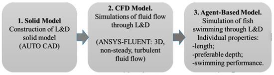
Figure 1.
Flow chart of stages used by the algorithm computational fluid dynamics agent-based (CFD-AB) model.
2.1. Fluid Equations
We consider three-dimensional incompressible fluid flow through a model channel with a tainter gate (Figure 2) which mimics the spillway portion of the typical Mississippi River LD. The computational region consists of a channel encased by the following boundaries: —bottom, top (i.e., water surface), left and right sides of the channel, inflow and outflow surfaces, and is the surface of the immersed tainter gate (Figure 2).
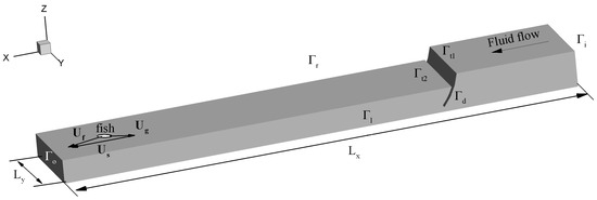
Figure 2.
Schematic model structure of a channel. The major surfaces of the computational region are: are the inflow and outflow surfaces; are left, right and top surfaces; is the surface of the gate, is the surface of the bottom (not shown). Vectors and are fluid velocity, ground velocity of a fish, and swimming speed of the fish, respectively.
The computational fluid mesh is generated by the ANSYS Mesh Editor and contains ~31,000 nodes with a minimum element edge length The solution of fluid flow in this computational region was obtained by FLUENT.
The Equations governing the motion of Newtonian incompressible fluid in the channel with geometry/surface of dam immersed in the fluid domain read as follows:
In the above Equations, is the mass density of the fluid, is the material or Lagrangian time derivative, is the fluid velocity and is the fluid stress tensor. The above Equations are subjected to Dirichlet and Neumann boundary conditions on all surfaces of the computational region:
Here, Equation (3) is the Dirichlet nonslip boundary conditions on the dam, bottom, right and left sides of the computational domain; Equation (4) is the inflow condition with prescribed velocity , which is defined from the known fluid discharge () and value of inflow surface area . Velocity at the inflow surface is equal to , is a unit vector coincided with the fluid flow direction; Equation (5) is a Neumann boundary which indicates the absence of stresses on the top of the water, and Equation (6) is the outflow boundary condition. Fluid flows around navigation dams are characterized by high turbulence conditions, and it is necessary to take into account the spatial distribution of turbulence. To solve fluid Equations (1)–(2) with ANSYS-FLUENT the Reynolds-Averaged Equations with the turbulence model [31] were used. The instantaneous fluid velocity can be written as , where is the mean velocity and is turbulent fluctuation of velocity.
The computational fluid dynamics (CFD) set-up (i.e., software package, mesh size, numerical solvers and turbulence closure) is consistent with that used by Zielinski et al. (2018) [4]. Zielinski et al. (2018) qualitatively validated the CFD model of LD8 with acoustic doppler current profiler (ADCP) surveys and a physical model study across seven different river discharge scenarios. By using a similar approach, the above CFD model is expected to resolve the major hydraulic features near a Mississippi River LD accurately.
2.2. Agent-Based Model
The Agent-Based fish passage model developed by Zielinski et al. (2018) [4] can be written as follows:
where , are the ground velocity and position/coordinate of the agent (e.g., fish), is the fatigue time defined by a relative swim speed (see below Equation (9), and (Figure 3). Fish swim upstream, i.e., in the coordinate system (Figure 2) its velocity will be negative, . The right-hand side of Equation (7) is a nonlinear abstract function which implicitly defines the acceleration of fish swimming from a known ground velocity, fluid velocity and swim speed to a fatigue time relationship generated from experimental swim tunnel data.
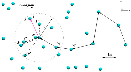
Figure 3.
This sketch explains the algorithm of upstream fish swimming (to simplify, we show a 2D Figure, which does not affect the generality of the 3D approach). Solid spheres are nodes of the fluid mesh generated by the ANSYS Mesh Editor. The current position of fish is a point ; is the radius of the searching algorithm; are points of a possible new fish location (i.e., neighboring nodes within the searching algorithm radius and positioned upstream of the current fish position) where the increment of fatigue is estimated, and is the new position of the fish, i.e., here, movement—red vector from point i to point that had caused the least fatigue. If for all directions , the next node is selected randomly.
Activity levels of fish swimming are defined by a swim speed to fatigue time relationship. Three basic modes of fish swimming are commonly recognized [32,33]: Sustainable, prolonged and burst swimming. In this paper, we only consider sustained and prolonged modes of swimming in bigheaded carp as experiments by Hoover et al. (2017) [21] could not distinguish between a prolonged and burst swimming mode. The prolonged mode can be defined based on the time for which a given speed can be maintained and read as:
where is the fatigue time (in minutes) and is the maximum sustainable swim speed. All velocities in Equation (11) and below are measured in body length per second (BL/s), otherwise we notice that the considered velocity is measured in meters per second (m/s). Fish can maintain swimming speeds less than the maximum sustainable swim speed indefinitely, and is conventionally defined as fatigue time . When fish swim at speeds greater than their maximum sustainable swim speed, they switch to the unsustainable prolonged (p) mode. The relationship between swim speed and fatigue time during prolonged mode swimming is characterized by coefficients in Equation (9). Castro-Santos (2005) [20] showed that for fish to overtake a velocity barrier using the least amount of energy, fish should swim at their theoretical distance-maximizing swim speed. According to this theory, fish swim with optimal ground speed , where is a fish’s speed relative to the ground (bottom of the channel). Hence, ground velocity, i.e., the velocity relative to the bottom of the channel, can be written as:
In the model, when fish swim at the sustained mode velocity, decreases when water velocity increases, and can become extremely low at . With further increasing water velocity , fish change to their prolonged swimming mode and maintain a constant ground speed .
2.2.1. Main Assumptions and Algorithm of the Agent-Based (AB) Model
- (a)
- The main assumptions of the original AB fish passage model used by Zielinski et al. (2018) [4] to simulate fish passing through a LD are as follows:
- (b)
- Fish only swim upstream;
- (c)
- fish swim in the direction that minimizes energy expenditure (minimal fatigue);
- (d)
- changes of fish velocity from a sustained mode to an unsustained (prolonged) speed and vice-versa are attached to the fluid velocity at the fish’s position (Equation (9));
- (e)
- at unsustainable swimming speeds, fish swim at a theoretical distance-maximizing ground speed (Equation (10));
- (f)
- fish try to maintain a species-specific depth that is determined using the best available data;
- (g)
- all fish swim until they pass through the dam or are completely exhausted.
During simulations, it takes no more than several minutes to reach the dam and pass through it. If the fish does not pass, it is assumed to be washed downstream, and cannot be used again because it can take several hours for fish to restore their energy [23], and these are viewed in the model as a new individual passage attempt.
Using Figure 3, we present a brief explanation of the original [1] AB algorithm, which describes successive steps of fish upstream movement in a known field of fluid flow (velocities). The fish in Figure 3 is assumed to be located at some node of the computational fluid mesh—, and selects the next step using the following algorithm:
Identification of closest nodes. Solid circles in Figure 3 are coordinates (nodes) of the 3D fluid computational mesh generated using the ANSYS Mesh Editor, and the fluid flow velocities , generated from solving Equations Equation (1)–Equation (8), are known at all nodes. Let us denote by and positions of fish on the previous and current time steps, respectively. In order to find the next coordinate position of the fish at, the searching algorithm is implemented to find nodes nearest to the fish, which are indicated in Figure 3 as. The selected nodes must be located in front of the current fish position and are close to the current fish position, i.e., , where is a vector connecting nodes and , and is a small length value for the searching algorithm. In the region close to the gate, where the mesh size is finest and the velocity gradients are likely the greatest ( downstream of the gates in this test case), the initial radius was set to half the total length of the fish, (approximately three times the minimum node spacing for the smallest modeled fish ).
In the region far from the dam, where the mesh size is coarse and velocity gradients are the lowest, the initial radius was equal to . The closest nodes located in the hemisphere will be found by searching all nodes of computational mesh . The searching algorithm is stopped when the number of nodes exceeds the maximum allowable number of nodes . If after the searching procedure there are either at least three nodes or no more than nodes, these nodes will be considered as the possible nodes of the next position of the fish. On the discussed example (Figure 3), there are six nodes in the hemisphere . In the original algorithm . If no nodes are located within the hemisphere radius after searching (), the radius will be increased as , and all nodes will be searched again.
Calculate resultant velocity at the selected nodes. In order to define the relative swim speed we use a resultant velocity , which is defined by analyzing directions of fluid velocity and possible fish displacement :
where ; , where is the coordinate of the water surface downstream of the gate (Figure 2), and is the preferable depth for specific species. Equation (11) essentially describes that when directions of velocity and displacement are the same, fish can swim to the particular node without spending energy, and hence in this direction is equal to zero, otherwise. For example, in the direction, because, according to the assumption of the algorithm, the fish always swims upstream ( see Figure 2), and
Definition of fish swimming mode. After the definition of velocities (Equation (11)) we can define the fish swimming mode. If the resultant velocity is rather small, i.e.,, the fish will swim at their maximum sustained speed. If the resultant velocity exceeds the maximum sustained swim speed, fish will switch from the sustained to prolonged swimming mode. We can define from Equation (10) and hence the relative swim speed. Note that because the direction of fluid flow and ground speed are opposite, the swimming speed of a fish will be higher than the fluid flow, and equal, for example, in the direction to. After the definition of ground speed for the all nearest nodes we can estimate the incremental fatigue fish must expend to reach each node.
Estimation of fatigue. The incremental fatigue fish must expend to reach nodes is defined [20] as
where , | are the time and distance swimming from the current to the next points, where is defined from Equation (9), and is a nondimensional value which is used as an indicator of incremental fatigue. Note that velocity is measured in (m/s). We use the same notation for velocity measured in (BL/s) (see, for example, Equation (10)) and here, and think it does not confuse readers. The next point is defined from. If for any of the nearest points,, then the next point is selected randomly from those points.
Updated final position and fatigue. The new position and fatigue of the fish at node is defined as:
So, when the fish reaches its fatigue limit and is considered completely exhausted. These ()() steps are repeated until the fish either reaches the opposite side of the dam (passes through the dam) or exhausts .
2.2.2. The Modification of the Original Algorithm of the Agent-Based Model
The original AB model [4] (Zielinski, et al., 2018) uses the nodes of the computational mesh from the CFD model to locate future fish positions. According to the algorithm, fish move from one mesh node to another. The solution of fluid Equations (1)–(8) depends on a dam structure, and hence on a computational fluid mesh. All LD structures vary in size and in geometry, which can influence the size and structure of the computational mesh used in the CFD model. We propose to use a special algorithm, allowing fish to be at any spatial position (not only at mesh nodes) by modifying the original version of the CFD-AB model, using smaller time steps in the integration of fish swimming Equations, which leads to smoother swimming trajectories of fish. It is demonstrated by solving a test problem of fish swimming in a channel (see below Section 3.1). Note, the proposed modifications of the original algorithm concerns only the computational aspect of the model, and its relation to actual swimming behavior is yet unknown. Close examination of the original algorithm revealed to heavily influence the fish swimming trajectory and passage index (see Section 3); therefore, we propose to modify the initial selection of and the position selection.
Identification of closest nodes. To make the CFD-AB approach independent of structure (mesh) size (for example, as we do it here by considering a small model part of a real LDs), we propose to select an initial radius for searching the closest nodes as . For the channel in Figure 2 , is a constant coefficient, which from our simulations (see Section 3) should be equal to . In the application at LD8, [1] set , and the initial radius was equal to half the total length of the fish close to the spillway gates, i.e., for fish. Using the proposed modification, the original algorithm utilized a constant equal to in the area close to the dam. Further away from the gates, the initial radius was equal to twice the total body length, i.e., , hence the constant was equal to . These two areas were separated ~ downstream of the spillway gates and distinguished as areas with fine and coarse mesh. Such separation could lead to erroneous pathway selections, because the mesh adaptively changed with the continual increasing/decreasing spatial step, and it is difficult to separate the computational region into two parts with strongly different spatial steps. Zielinski et al. (2018) [4] used this approach to simply reduce the computational time because the large mesh spacing away from the spillway gates required repeated searches through the mesh to locate more than three nodes within the initial search region. Selection of ensures fish locate the closest mesh nodes in any point of the computational region where fish are positioned. This value of is utilized for all of the computational region. If the computational mesh employs uniform, multi-block meshes, it would be possible to separate the computational region into different sub-regions with specific and. Such actions allow the selection of the closest nodes to the fish position while minimizing the possibility of bypassing nodes defining large velocity gradients. We also found that is a good selection for the collected max number of nodes in the hemisphere . Increasing this number increases computational resources, but does not change the final results with fish passage (see Section 3).
Steps (II) and (III) remain unchanged for the modified algorithm. Following step (III), rather than shift the fish to the next computational mesh node, we allow the fish to move in the direction of least fatigue for a pre-specified duration. We define a unit vector as the direction of fish advancing: . Fish swims along the unit vector with a smaller displacement according to a smaller time step. Figure 4 demonstrates how a fish, starting at position #1, moves through a computational region with uniform time steps (pink circles). The computational node chosen by the search algorithm sets the direction of movement (dashed arrows).
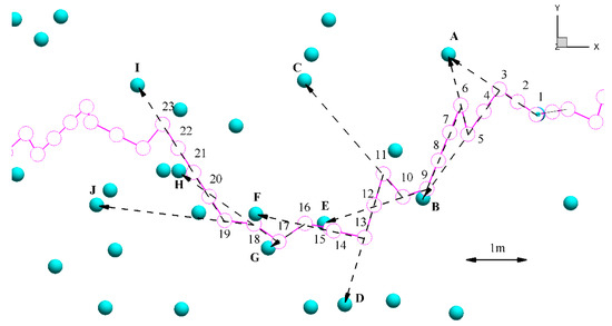
Figure 4.
Movement path of a fish using the modified algorithm. Numbers (pink circles) #1–#23 are indicators of fish positions. Letters A–J (light blue spheres) indicate nodes of the computational mesh. Dashed arrows indicate the direction of movement, and point towards the computational node used to calculate fluid, ground and swimming velocity.
Instead of step () the next step () is implemented.
() Estimation of fatigue. The incremental fatigue of the fish at the next node is defined as:
where is a time step for fish swimming (Equations (7)8)), which is smaller than the average time step in the original algorithm (Equation (12)), is the incremental fatigue accrued while fish swim in the direction .The next point is defined as in from
Updated final position and fatigue. The coordinates of fish position and total fatigue are defined as:
2.3. Comparison of Methods
We compared the original and modified algorithms by simulating an upstream passage of fish through a simplified channel with a tainter gate raised off the channel bottom. To construct the simplified channel we have taken only one part of the real LD 5 with the tainter gate, but instead of the real bathymetry, a simple flat bottom was used. The swimming performance parameters of fish trying to pass through the gate were chosen for bighead carp (Zielinski, et al., 2018 [4]): , . In our simulations, the size of bighead carp is , the preferable depth is Equal to , and the initial total number of fish starting to swim upstream is equal to 100. In order to estimate the mean and standard deviation of the fish passage index, the calculations were repeated 10 times.
In the original algorithm, the time step is dependent upon the computational mesh and ground velocity (Equation (14)) which are changing. Far from the gate where the mesh is coarser, the time step is bigger than in close proximity to the gate where the mesh is finer. For example, oscillations of the time step (Figure 5) mostly occur due to changes in the distance swam between mesh nodes. Examining the time step selection of a fish moving through the test case, the time step changes from a minimum to maximum value , with a mean value of (Figure 5). This observation, along with reaction times documented for fish responding to hydrodynamic disturbances [34], prompted us to simulate fish pathways using the modified approach with time steps set at and

Figure 5.
Dependence of time step versus the distance of fish movement for the original approach.
2.3.1. Role of and in Algorithm Performance
To demonstrate the improvement of the modified algorithm over the original algorithm, we begin by evaluating the role of parameters and in the original searching algorithm performance and their impact on estimates of fish passage. These parameters were introduced in (I) Identification of closest nodes. While it is intuitively clear that reductions in the initial hemisphere radius will provide a selection of nodes closest to the fish, it will also require many more calculations of fish swimming steps, and drastically increase computational time. To obtain the optimal (from the point of view of minimizing computer time) value of we simulated fish passage through the simplified domain using the initial radius , with To investigate the dependence of %FPI from changing the maximum number of nodes in sphere (Figure 3), we also simulated the test case with .
2.3.2. Influence of Discharge
To estimate how changes with increasing input flow velocity , we varied input velocities . Although it is evident that by increasing flow discharge through the channel the fish passage will decrease, but it is not known quantitatively how fast it will go down. Our simulations show that such decreasing will go down exponentially with increasing flow discharge.
2.3.3. Pathway Characteristics
To compare the smoothness, defined as a measure of pathway variability and direction change, the maximum deviation of the pathways from two types of linear functions were calculated for the original and modified algorithm.
Linear functions formed using the standard least-squares method to approximate the fish’s pathway were constructed for the original and three cases of the modified algorithm. Because the linear functions do not fit all pathway curves well, a second set of approximations were generated using a LOWESS smoother [35].
3. Results
To demonstrate the utility of the modified algorithm, comparative simulations of fish swimming in a model channel for the original CFD-AB and modified approaches are shown in Figure 6. The flow field contains a large recirculation zone downstream of the tainter gate (Figure 6a). Trajectories displayed in Figure 6b–e demonstrate similar pathways across all algorithm settings, but the modified approach using a step size of 0.1 s produces a pathway with less variability and reduced direction changes. Pathway solutions for the original and modified algorithm were obtained using the same parameters and with a gradually decreasing time step. As a result of the smoother pathway, fish swimming trajectories calculated by the modified algorithm also reduce the required energy expended. The reason is that with a smaller time step, fish adjust to the flow and try to swim into the recirculation zone by using vortex energy (Figure 6c–e). Fish swim without spending energy within the recirculation zone because the water velocity direction coincides with the fish trajectory.
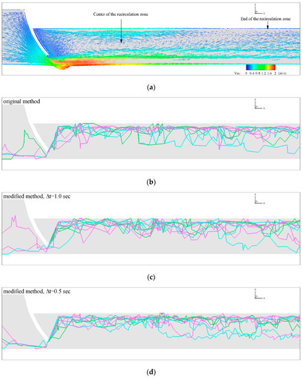
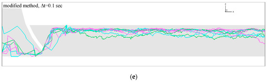
Figure 6.
Pathway of fishes for the original and modified agent-based (AB) method. (a) Velocity vectors of fluid flow showing the generation of a big circulation zone behind the tainter gate. Colors indicate the magnitude of the velocities. The center and the end of the circulation zone are shown with arrows. (b) Fishes pathway of the original algorithm and (c–e) of the modified algorithm with (c) , (d) and (e) . To facilitate the visual view of the fishes pathway only 10 of the simulated 100 fishes are shown here.
3.1. Role of and in Algorithm Performance for
The fish passage index %FPI with , and are shown in Figure 6. While results with and are very similar (Figure 7a), increasing the initial searching radius of with and gives results presented in Figure 7b,c, respectively, that are significantly higher than in Figure 7a. A larger sphere allows nodes closer to the fish to be ignored, and preference is given to nodes far from the fish with . Hence, more fish in this case will be able to pass through the gate. We note that increasing fish passage with increasing occurs both for the original and modified algorithm as it is seen from Figure 7b,c. Further increasing results in one hundred percent of fish passage, i.e., %FPI = 100.
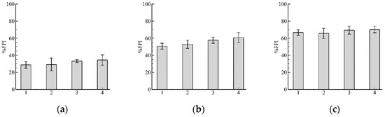
Figure 7.
Results of fish passage index (%FPI) with varying: (a) ; (b) and (c) . The numbers of the abscissa indicate bars 1, 2, 3 and 4, where 1 refers to the original algorithm, 2, 3 and 4 refer to the modified algorithm with , , and s, respectively. These results clearly show that increasing the initial radius in the searching algorithm leads to increases to %FPI, and hence to errors in the estimation of the fish passage.
Analyzing the differences of %FPI between the original and modified algorithm (Figure 7a) show that the values of the fish passage index of the modified algorithm are larger. Calculations of relative errors give the values: where Here is the fish passage index for the original algorithm, and is the fish passage index for the updated algorithm with time step ∆t. We can visually estimate from Figure 7a that with decreasing the time step the fish passage index %FPI is slowly increased and converged to the level .
The fish passage index %FPI for , are shown in Figure 8. It is clearly seen that the mean values of %FPI do not change visibly by increasing , which is logical because guarantees that nodes closest to the current fish position are selected. Reducing the number of nodes from to leads to a reduction in computational time by half. From these results, we can make a conclusion that is sufficient to provide simulations of fish swimming.
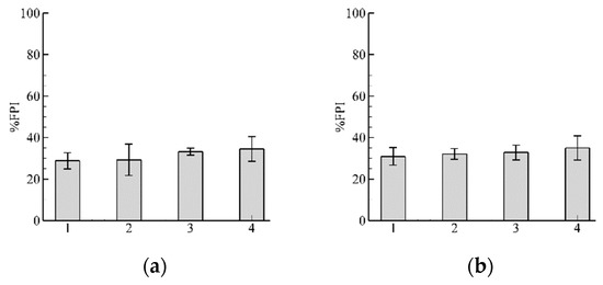
Figure 8.
Results of fish passage index %FPI for and two different closest to fish position nodes: (a) and (b) . It is clearly seen that the mean values of %FPI do not change by increasing , which is reasonable, because guarantees that nodes closest to the current fish position are selected. From these results, we can make a conclusion that is sufficient to provide simulations of fish swimming. The numbers of the abscissa indicate bars with the same meaning as in Figure 7.
3.2. Influence of Discharge
Results with and are shown in Figure 9a,b, respectively. With increasing input flow the decreases (Figure 9b). Further increasing leads to an almost complete blockage of the fish passage ).
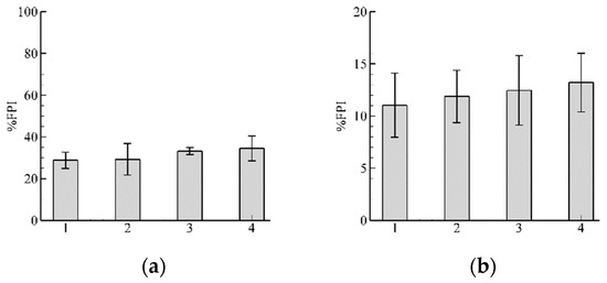
Figure 9.
Results of %FPI for two different flow discharges: (a) Inflow ; (b) . Results with leads to an almost complete blockage of fish passage ), and does not show here. Note that scales for (a,b) are different and Equal to 100% and 20%, respectively.
3.3. Pathway Characteristics
The results of max deviations of fish’s pathway from appropriate linear functions were defined and are shown in Table 1 (first row).

Table 1.
Maximum deviations for original () and modified ( algorithms.
Note that . for the modified algorithm is bigger than of the original algorithm (). It is explainable by the fact that in the considered area close to the gate, the mesh is fine, and the time step for the original algorithm is less than the time step for the modified algorithm s (see Figure 5). The results with the implementation of the LOWESS smoother (α = 0.5) are shown in Table 1 (second row). Comparisons of the two approximations show that the max deviations of the LOWESS smoother are smaller than in case of the linear function, and both linear and our LOWESS functions indicate the modified algorithm provides a smoother fish pathway in comparison to the original approach based upon the max deviation analysis.
4. Discussion
The proposed modified algorithm improves the CFD-AB model of Zielinski, et al. (2018) [4] by setting a constant movement time step , which allows fish to occupy any location in the computational domain. Changing the time step and fish position selection alters the fish passage index results from the original and approaches by 2–16% (Figure 7a). The proposed modification of the CFD-AB algorithm provides smoother fish swimming trajectories which reduces mesh dependency and further improves the models search algorithm seeking the least energetic path. In Figure 6b–e are clearly seen the qualitative comparisons of fishes pathway for the original and modified approaches. It is seen that already from the pathway of the modified becomes smoother.
Using the flow features with vortex formation (Figure 6a) fishes save their energy, which gives them a possibility to pass through the gate. Although it is known that “fish appear to use very large eddies as conveyor belts for migration” [36], it does not mean that we present and argue biological fish behavior. We only use the idea of the least fatigue, and it seems that according to this idea when fish moves with a smaller time step at a smaller distance, it finds a way to save energy.
In conclusion, a modified approach for the Zielinski et al. (2018) [4] CFD-AB model describing fish passage through LDs has been developed. In the original algorithm, the freedom to find the direction of fish swimming is restricted by an existing computational mesh, which in some areas of the domain can be rather coarse. The modified algorithm with decreasing time step gives fish more freedom in the simulation to move to any point in the domain that can be reached within a defined time step, not necessarily coinciding with the mesh nodes. The modification of the original algorithm by using the decreasing of the time step provides minimizing mesh dependency, and gives the maximum difference for fish passage equal to 16% between the original and modified approaches. We also showed that the modified algorithm gives the smoother fish pathway that is based on qualitative and quantitative comparisons.
It is well known that silver carp, in some cases, demonstrate spectacular leaping abilities, which could be used to overcome areas of high water velocity. One of the possible future developments of the CFD-AB approach is to take jumping into account (e.g., incorporate a ballistic model approach similar to Powers and Osborn (1985) [37]), which would require a substantial expenditure of energy, but would also have major benefits in terms of bypassing areas of very high water velocity.
Author Contributions
Conceptualization, A.G., D.Z.; methodology, A.G., D.Z., V.V; software, A.G., D.Z.; validation, A.G.; formal analysis, A.G., D.Z., V.V.; investigation, A.G.; writing—original draft preparation, A.G.; writing—review and editing, A.G., D.Z., V.V., P.S.; visualization, A.G.
Funding
This work was done with Funding from the Environment and Natural Resources Trust Fund in association with the Minnesota Aquatic Invasive Species Research Center.
Acknowledgments
The computational simulation was done on the Supercomputer Institute of Minnesota.
Conflicts of Interest
The authors declare no conflict of interest.
References
- Larson, J.H.; Knights, B.C.; McCalla, S.G.; Monroe, E.; Tuttle-Lau, M.; Chapman, D.C.; George, A.E.; Vallazza, J.M.; Amberg, J. Evidence of Asian Carp Spawning Upstream of a Key Choke Point in the Mississippi River. North Am. J. Fish. Manag. 2017, 37, 903–919. [Google Scholar] [CrossRef]
- Kokotovich, A.; Andow, D.; Aadland, L.; Bertrand, K.; Coulter, A.; Frohnauer, N.; Hoff, M.; Hoxmeier, J.; O’Hara, M.; Phelps, Q.; et al. Minnesota Bigheaded Carps Risk Assessment; Minnesota Department of Natural Resource: Saint Paul, MN, USA, 2017. [Google Scholar]
- Upper Mississippi River Asian Carp Partnership. Upper Mississippi River Basin Asian Carp Control Strategy Framework; Jackson, N., Runstrom, A., Eds.; Upper Mississippi River Conservation Committee Fisheries Technical Section: Marion, IL, USA, 2018; p. 13. [Google Scholar]
- Zielinski, D.P.; Voller, V.R.; Sorensen, P.W. A physiologically inspired agent-based approach to model fish swimming fatigue and its application to upstream passage of invasive fish at a lock and dam. Ecol. Modeling 2018, 382, 18–32. [Google Scholar] [CrossRef]
- Knights, B.C.; Vallazza, J.M.; Zigler, S.J.; Dewey, M.R. Habitat and movement of lake sturgeon in the upper Mississippi River system. USA Trans. Am. Fish. Soc. 2002, 131, 507–522. [Google Scholar] [CrossRef]
- Zigler, S.J.; Dewey, M.R.; Knights, B.C.; Runstrom, A.L.; Steingraeber, M.T. Movement and habitat use by radio-tagged paddlefish in the upper Mississippi River and tributaries. North Am. J. Fish. Manag. 2003, 23, 189–205. [Google Scholar] [CrossRef]
- Hussey, N.E.; Kessel, S.T.; Aarestrup, K.; Cooke, S.J.; Cowley, P.D.; Fisk, A.T.; Whoriskey, F.G. Aquatic animal telemetry: A panoramic window into the underwater world. Science 2015, 348, 1255642. [Google Scholar] [CrossRef]
- Kessel, S.T.; Cooke, S.J.; Heupel, M.R.; Hussey, N.E.; Simpfendorfer, C.A.; Vagle, S.; Fisk, A.T. A review of detection range testing in aquatic passive acoustic telemetry studies. Rev. Fish Biol. Fish. 2014, 24, 199–218. [Google Scholar] [CrossRef]
- Silva, A.T.; Lucas, M.C.; Castro-Santos, T.; Katopodis, C.; Baumgartner, L.J.; Thiem, J.D.; Aarestrup, K.; Pompeu, P.; O’Brien, G.C.; Braun, D.C.; et al. The future of fish passage science, engineering, and practice. Fish Fish. 2018, 19, 340–362. [Google Scholar] [CrossRef]
- Castro-Santos, T.; Haro, A. Fish guidance and passage at barriers. In Fish Locomotion: An Eco-Ethological Perspective; Domenici, P., Kapoor, B.G., Eds.; Science Publishers: Enfield, NH, USA, 2010; pp. 62–89. [Google Scholar]
- McElroy, B.; Delonay, A.; Jacobson, R. Optimum swimming pathways of fish spawning migrations in rivers. Ecology 2012, 93, 29–34. [Google Scholar] [CrossRef]
- Thiem, J.D.; Dawson, J.W.; Hatin, D.; Danylchuk, A.J.; Dumont, P.; Gleiss, A.C.; Wilson, R.P.; Cooke, S.J. Swimming activity and energetic costs of adult lake sturgeon during fishway passage. J. Exp. Biol. 2016, 219, 2534–2544. [Google Scholar] [CrossRef]
- Hammer, C. Fatigue and exercise tests with fish. Comp. Biochem. Physiol. Part A 1995, 112, 1–20. [Google Scholar] [CrossRef]
- Plaut, I. Critical swimming speed: Its ecological relevance. Comp. Biochem. Physiol. Part A 2001, 131, 41–50. [Google Scholar] [CrossRef]
- Wardle, C.S.; He, P. Burst swimming speeds of mackerel. J. Fish Biol. 1988, 32, 471–478. [Google Scholar] [CrossRef]
- Bainbridge, R. Speed and stamina in three fish. J. Exp. Biol. 1960, 37, 129–153. [Google Scholar]
- Beamish, F.W.H. Swimming performance of three southwest Pacific fishes. Mar. Biol. 1984, 79, 311–313. [Google Scholar] [CrossRef]
- Dorn, P.; Johnson, L.; Darby, C. The swimming performance of nine species of common California in-shore fishes. Trans. Am. Fish. Soc. 1979, 108, 366–372. [Google Scholar] [CrossRef]
- Videler, J.J. Fish Swimming; Chapman & Hall: London, UK, 1993. [Google Scholar]
- Castro-Santos, T. Optimal swim speeds for traversing velocity barriers: An analysis of volitional high-speed swimming behavior of migratory fishes. J. Exp. Biol. 2005, 208, 421–432. [Google Scholar] [CrossRef]
- Hoover, J.J.; Zielinski, D.P.; Sorensen, P.W. Swimming performance of adult silver and bighead carp. J. Appl. Ichth. 2017, 33, 54–62. [Google Scholar] [CrossRef]
- Davison, W. The effects of exercise training on teleost fish, a review of recent literature. Comp. Biochem. Physiol. Part A Physiol. 1997, 117, 67–75. [Google Scholar] [CrossRef]
- Kieffer, J.D. Limits to exhaustive exercise in fish. Comp. Biochem. Physiol. Part A Mol. Integr. Physiol. 2000, 126, 161–179. [Google Scholar] [CrossRef]
- Goodwin, R.A.; Nestler, J.M.; Anderson, J.J.; Weber, L.J.; Loucks, D.P. Forecasting 3-D fish movement behavior using a Eulerian–Lagrangian–agent method (ELAM). Ecol. Model. 2006, 192, 197–223. [Google Scholar] [CrossRef]
- Smith, D.L.; Goodwin, R.A.; Nestler, J.M. Relating turbulence and fish habitat: A new approach for management and research. Rev. Fish. Sci. Aquac. 2014, 22, 123–130. [Google Scholar] [CrossRef]
- Haefner, J.W.; Bowen, M.D. Physical-based model of fish movement in fish extraction facilities. Ecol. Model. 2002, 152, 227–245. [Google Scholar] [CrossRef]
- Arenas, A.; Politano, M.; Weber, L.; Timko, M. Analysis of movements and behavior of smolts swimming in hydropower reservoirs. Ecol. Modeling 2015, 312, 292–307. [Google Scholar] [CrossRef]
- Eiler, J.H.; Evans, A.N.; Schreck, C.B. Migratory Patterns of Wild Chinook Salmon Oncorhynchus tshawytscha Returning to a Large, Free-Flowing River Basin. PLoS ONE 2015, 10, e0123127. [Google Scholar]
- Furniss, M.; Love, M.; Firor, S.; Moynan, K.; Llanos, A.; Guntle, J.; Gubernick, R. FishXing: Software and Learning Systems for Fish Passage Through Culverts, Version 3.0. U.S. Forest Service; San Dimas Technology and Development Center: San Dimas, CA, USA, 2006. [Google Scholar]
- Gao, Z.; Andersson, H.I.; Dai, H.; Jiang, F.; Zhao, L. A new Eulerian-Lagrangian agent method to model fish paths in a vertical slot fishway. Ecol. Eng. 2016, 88, 217–225. [Google Scholar] [CrossRef]
- Spalart, P.R. Strategies for turbulence modelling and simulations. Int. J. Heat Fluid Flow 2000, 21, 252–263. [Google Scholar] [CrossRef]
- Brett, J.R. The respiratory metabolism and swimming performance of young sockeye salmon. J. Fish. Res. Bd. Can. 1964, 21, 1183–1226. [Google Scholar] [CrossRef]
- Brett, J.R. Swimming performance of sockeye salmon in relation to fatigue time and temperature. J. Fish. Res. Board Can. 1967, 24, 1731–1741. [Google Scholar] [CrossRef]
- Webb, P.W. Response latencies to postural disturbances in three species of teleostean fishes. J. Exp. Biol. 2004, 207, 955–961. [Google Scholar] [CrossRef]
- Cleveland, W.S.; Grosse, E.; Shyu, W.M. Local regression models. In Chapter 8 of Statistical Models in S; Chambers, J.M., Hastie, T.J., Eds.; Wadsworth & Brooks/Cole: Berlin/Heidelberg, Germany, 1992. [Google Scholar]
- Webb, P.W.; Cotel, A.J.; Meadows, L.A. Waves and eddies: effects on fish behaviour and habitat distribution. In Fish Locomotion: An Eco-ethological Perspective; Domenici, P., Kapoor, B.G., Eds.; Science Publishers: Enfield, NH, USA, 2010; pp. 1–39. [Google Scholar]
- Powers, P.D.; Osborn, J.F. Analysis of Barrier to Upstream Fish Migration; Contract DE-A179-82BP36523, Project 82-14; Albrock Hydraulics Laboratory: Pullman, WA, USA, 1985. Available online: http://www.efw.bpa.gov/Publications/U36523–1.pdf (accessed on 1 July 2019).
© 2019 by the authors. Licensee MDPI, Basel, Switzerland. This article is an open access article distributed under the terms and conditions of the Creative Commons Attribution (CC BY) license (http://creativecommons.org/licenses/by/4.0/).