A Cautionary Note on the Reproduction of Dependencies through Linear Stochastic Models with Non-Gaussian White Noise

 , ,
, , 

Abstract
1. Introduction: A Glimpse of History
“Remember that all models are wrong; the practical question is how wrong do they have to be to not be useful.”—George Box and Norman Draper [1]
2. The Envelope Behavior of Linear Stochastic Models with Non-Gaussian White Noise
2.1. The Thomas-Fiering Approach
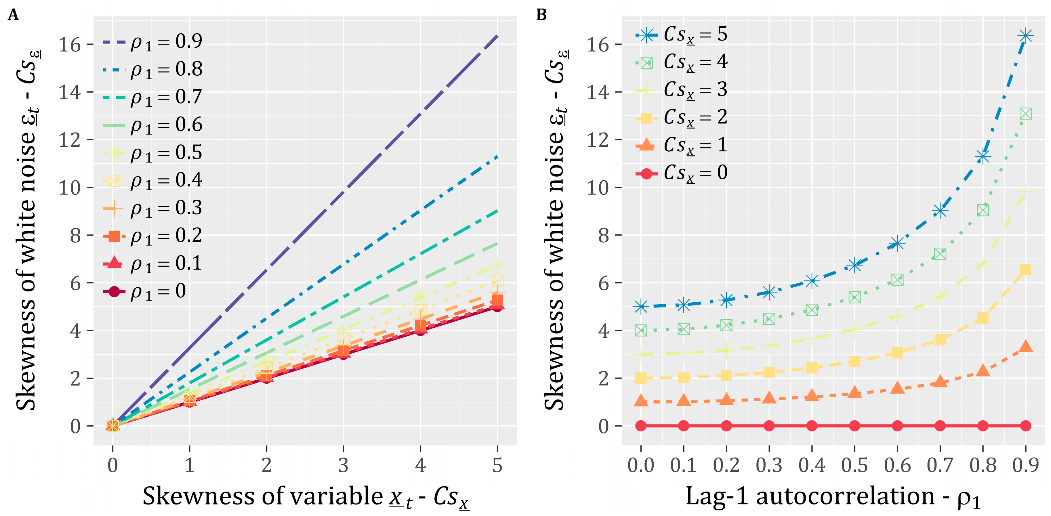
2.2. The Envelope Behavior in the Classical Univariate AR(1) Model
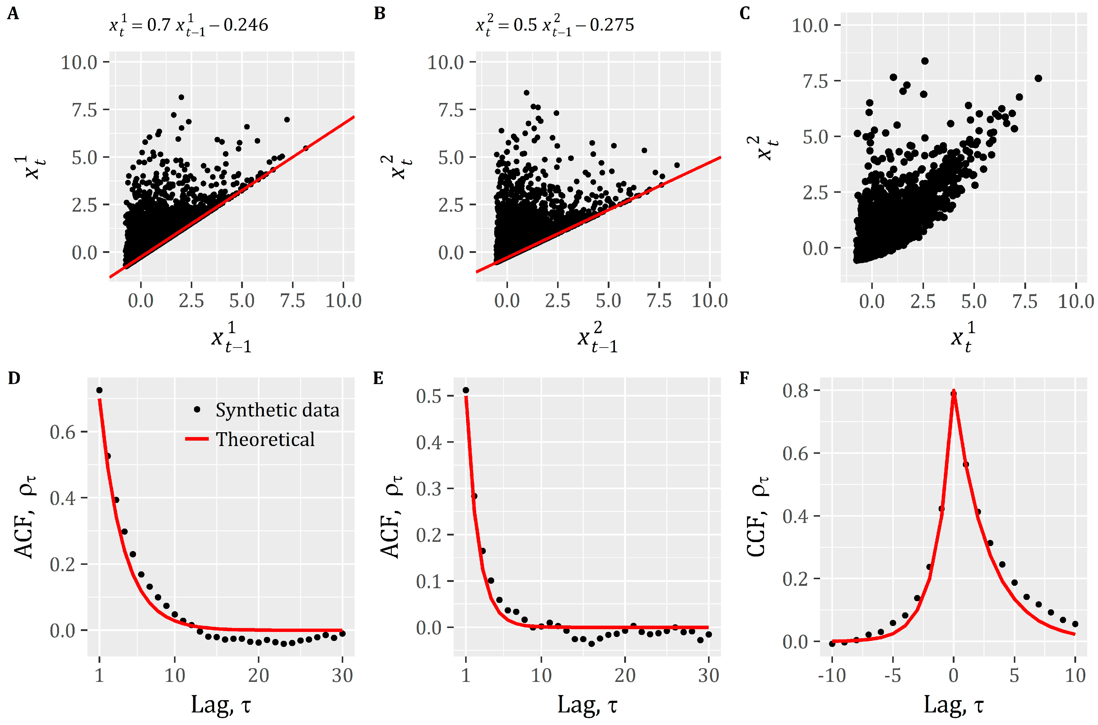
2.3. From the Univariate to the Multivariate AR(1) Model
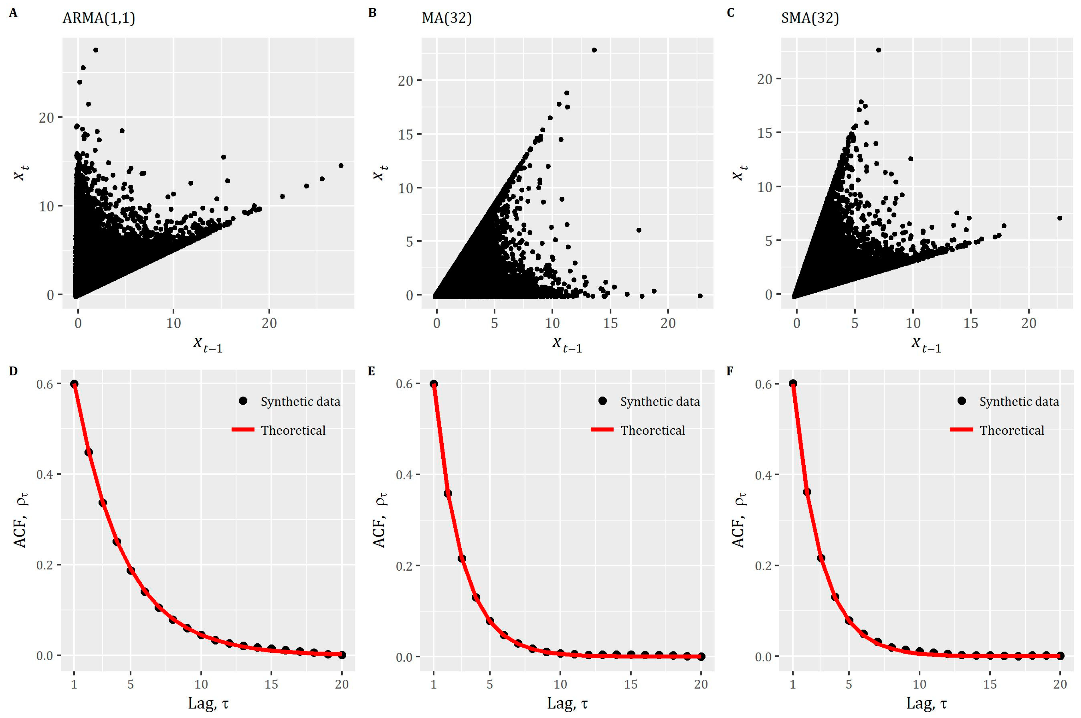
2.4. The Envelope Behavior beyond AR Models
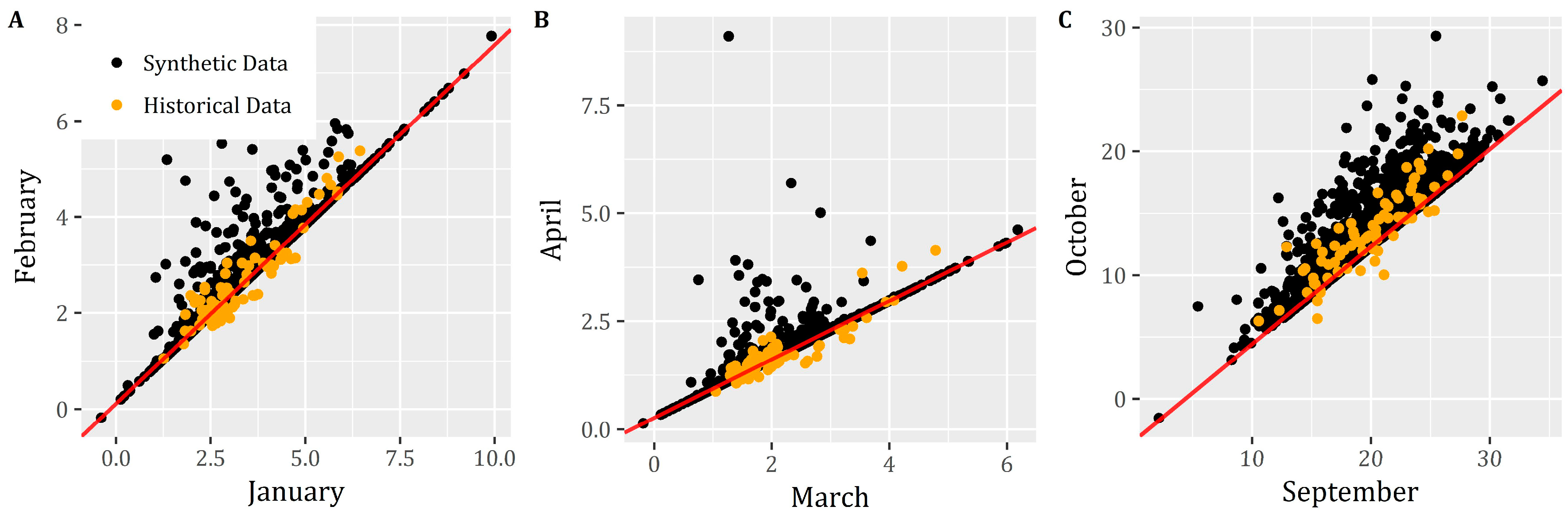
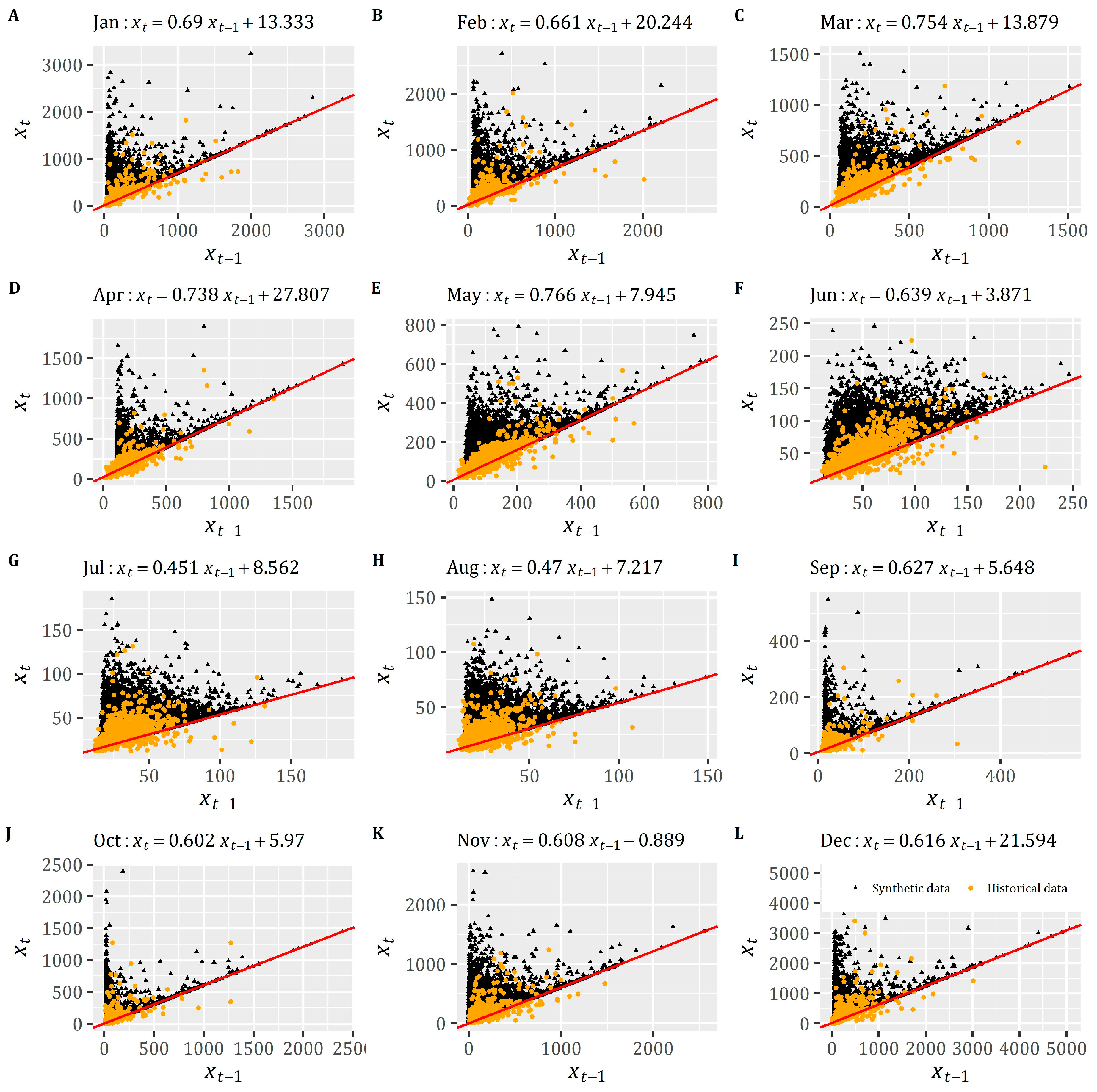
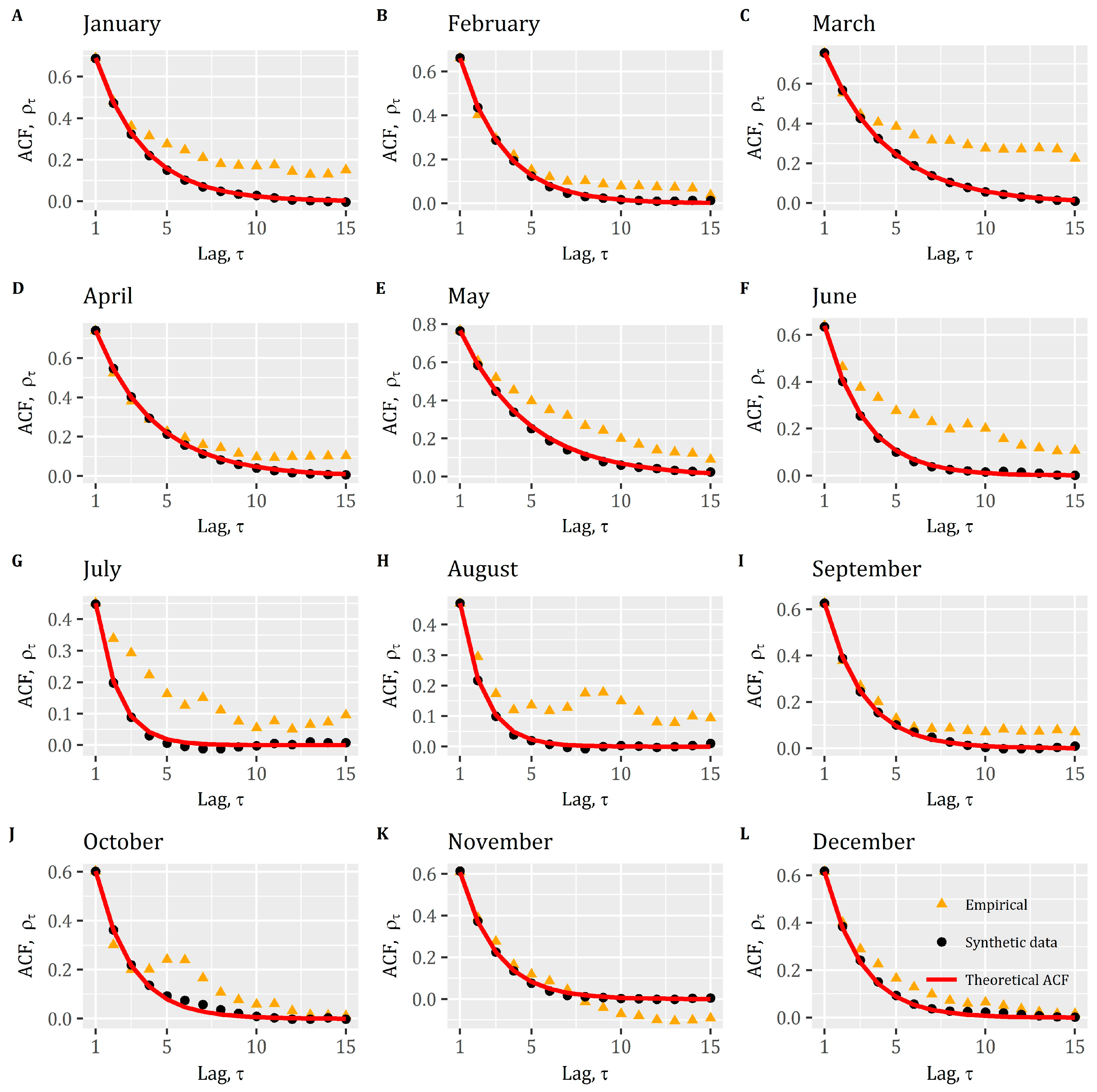
3. Real-World Case Study
4. Discussion
5. Conclusions
Author Contributions
Acknowledgments
Conflicts of Interest
Appendix A
Appendix B

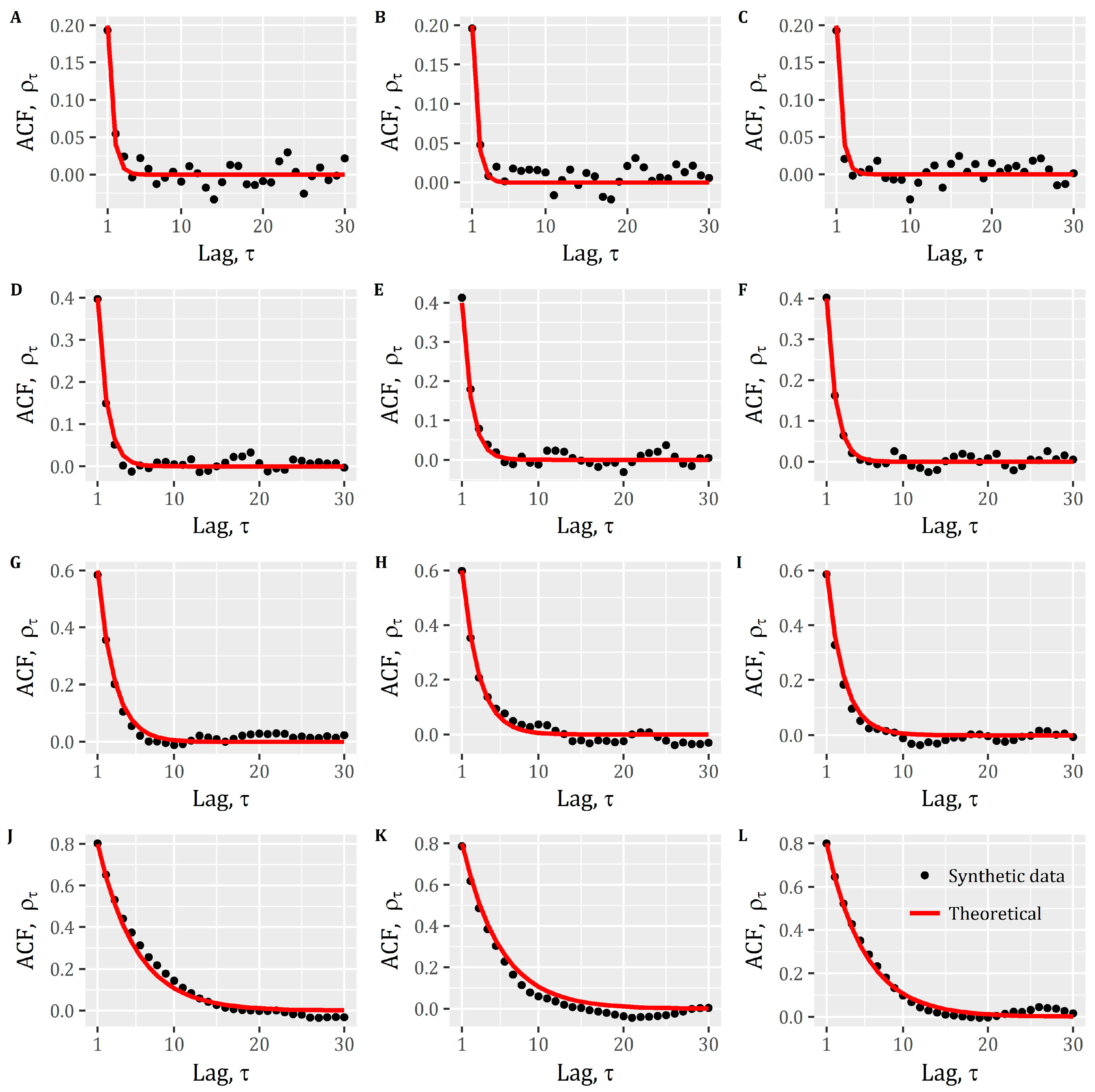
| Scenario | Type | Mean (μ) | Variance (σ2) | Skewness (Cs) | Autocorrelation (ρ1) |
|---|---|---|---|---|---|
| Scenario A | Theoretical | 0.50 | 1.00 | 1.00 | 0.20 |
| Simulated | 0.46 | 0.93 | 1.05 | 0.20 | |
| Scenario B | Theoretical | 0.50 | 1.00 | 2.00 | 0.20 |
| Simulated | 0.54 | 1.06 | 2.07 | 0.18 | |
| Scenario C | Theoretical | 0.50 | 1.00 | 4.00 | 0.20 |
| Simulated | 0.50 | 0.91 | 3.48 | 0.21 | |
| Scenario D | Theoretical | 0.50 | 1.00 | 1.00 | 0.40 |
| Simulated | 0.46 | 0.97 | 0.91 | 0.34 | |
| Scenario E | Theoretical | 0.50 | 1.00 | 2.00 | 0.40 |
| Simulated | 0.49 | 1.11 | 2.09 | 0.45 | |
| Scenario F | Theoretical | 0.50 | 1.00 | 4.00 | 0.40 |
| Simulated | 0.46 | 1.01 | 4.89 | 0.45 | |
| Scenario G | Theoretical | 0.50 | 1.00 | 1.00 | 0.60 |
| Simulated | 0.42 | 0.97 | 0.88 | 0.64 | |
| Scenario H | Theoretical | 0.50 | 1.00 | 2.00 | 0.60 |
| Simulated | 0.48 | 1.04 | 2.20 | 0.62 | |
| Scenario I | Theoretical | 0.50 | 1.00 | 4.00 | 0.60 |
| Simulated | 0.48 | 0.93 | 4.22 | 0.57 | |
| Scenario J | Theoretical | 0.50 | 1.00 | 1.00 | 0.80 |
| Simulated | 0.50 | 1.09 | 0.75 | 0.82 | |
| Scenario K | Theoretical | 0.50 | 1.00 | 2.00 | 0.80 |
| Simulated | 0.45 | 0.97 | 2.11 | 0.81 | |
| Scenario L | Theoretical | 0.50 | 1.00 | 4.00 | 0.80 |
| Simulated | 0.55 | 1.08 | 4.24 | 0.81 |

| Process | Type | Mean (μ) | Variance (σ2) | Skewness (Cs) | Autocorrelation (ρ1) |
|---|---|---|---|---|---|
| Theoretical | 0.50 | 1.00 | 2.00 | 0.00 | |
| Simulated | 0.50 | 1.06 | 2.39 | 0.00 | |
| Theoretical | 0.50 | 1.00 | 2.50 | 0.00 | |
| Simulated | 0.51 | 1.14 | 2.95 | 0.00 | |
| Theoretical cross-correlation (ρ0) = 0.80|Simulated cross-correlation (ρ0) = 0.79 | |||||
| Process | Type | Mean (μ) | Variance (σ2) | Skewness (Cs) | Autocorrelation (ρ1) |
|---|---|---|---|---|---|
| Theoretical | 0.50 | 1.00 | 2.00 | 0.70 | |
| Simulated | 0.52 | 1.08 | 2.00 | 0.70 | |
| Theoretical | 0.50 | 1.00 | 2.50 | 0.50 | |
| Simulated | 0.52 | 1.11 | 2.51 | 0.51 | |
| Theoretical cross-correlation (ρ0) = 0.80|Simulated cross-correlation (ρ0) = 0.80 | |||||
| Month | Type | Mean (μ) | Variance (σ2) | Skewness (Cs) | Autocorrelation (ρ1) |
|---|---|---|---|---|---|
| January | Historical | 167.89 | 33,973.86 | 3.89 | 0.69 |
| Simulated | 166.12 | 35,044.58 | 3.92 | 0.70 | |
| February | Historical | 179.50 | 32,317.25 | 3.95 | 0.66 |
| Simulated | 177.10 | 32,538.62 | 4.28 | 0.66 | |
| March | Historical | 172.07 | 13,773.37 | 2.69 | 0.75 |
| Simulated | 173.37 | 13,608.23 | 2.68 | 0.75 | |
| April | Historical | 172.47 | 10,253.59 | 4.04 | 0.74 |
| Simulated | 171.62 | 10,502.08 | 4.28 | 0.74 | |
| May | Historical | 107.83 | 4055.14 | 2.29 | 0.77 |
| Simulated | 110.20 | 4368.32 | 2.31 | 0.77 | |
| June | Historical | 50.86 | 591.95 | 1.59 | 0.64 |
| Simulated | 51.26 | 604.55 | 1.58 | 0.63 | |
| July | Historical | 31.13 | 177.42 | 2.19 | 0.45 |
| Simulated | 31.06 | 176.04 | 2.17 | 0.45 | |
| August | Historical | 24.00 | 96.04 | 2.41 | 0.47 |
| Simulated | 23.96 | 94.83 | 2.35 | 0.47 | |
| September | Historical | 24.86 | 492.39 | 5.99 | 0.63 |
| Simulated | 24.42 | 432.84 | 5.57 | 0.63 | |
| October | Historical | 51.77 | 8883.06 | 6.70 | 0.60 |
| Simulated | 50.71 | 7905.46 | 6.26 | 0.60 | |
| November | Historical | 114.63 | 24,332.88 | 3.49 | 0.61 |
| Simulated | 111.69 | 23,039.17 | 3.63 | 0.61 | |
| December | Historical | 197.14 | 68,785.55 | 4.87 | 0.62 |
| Simulated | 193.85 | 63,948.33 | 4.53 | 0.61 |

References
- Box, G.E.P.; Draper, N.R. Empirical Model-Building and Response Surfaces; Wiley: New York, NY, USA, 1987; Volume 424, p. 74. [Google Scholar]
- Maass, A.; Hufschmidt, M.M.; Dorfman, R.; Thomas, H.A.; Marglin, S.A.; Fair, G.M.; Bower, B.T.; Reedy, W.W.; Manzer, D.F.; Barnett, M.P. Design of Water-Resource Systems; Harvard University Press: Cambridge, UK, 1962. [Google Scholar]
- Fiering, B.; Jackson, B. Synthetic Streamflows (Water Resources Monograph); American Geophysical Union: Washington, DC, USA, 1971; Volume 1, ISBN 0-87590-300-2. [Google Scholar]
- Thomas, H.A.; Fiering, M.B. Mathematical synthesis of streamflow sequences for the analysis of river basins by simulation. In Design of Water Resources-Systems; Harvard University Press: Cambridge, UK, 1962; pp. 459–493. [Google Scholar]
- Fiering, M.B. Streamflow Synthesis; Harvard University Press: Cambridge, UK, 1967; p. 139. [Google Scholar]
- Jackson, B.B. The use of streamflow models in planning. Water Resour. Res. 1975, 11, 54–63. [Google Scholar] [CrossRef]
- Matalas, N.C. Mathematical assessment of synthetic hydrology. Water Resour. Res. 1967, 3, 937–945. [Google Scholar] [CrossRef]
- Hirsch, R.M. Synthetic hydrology and water supply reliability. Water Resour. Res. 1979, 15, 1603–1615. [Google Scholar] [CrossRef]
- Klemeš, V. Water storage: Source of inspiration and desperation. In Reflections on Hydrology: Science and Practice; American Geophysical Union: Washington, DC, USA, 1997; pp. 286–314. ISBN 9781118668085. [Google Scholar]
- Loucks, D.P.; van Beek, E. An Introduction to Probability, Statistics, and Uncertainty. In Water Resource Systems Planning and Management; Springer: Berlin, Germany, 2017; pp. 213–300. [Google Scholar]
- Kottegoda, N.T. Stochastic Water Resources Technology; Palgrave Macmillan: London, UK, 1980; ISBN 1349034673. [Google Scholar]
- Reddy, P.J.R. Stochastic Hydrology; Laxmi Publications, Ltd.: New Delhi, India, 1997; ISBN 817008086X. [Google Scholar]
- Bras, R.L.; Rodríguez-Iturbe, I. Random Functions and Hydrology; Addison-Wesley, Reading, Mass: Boston, MA, USA, 1985; ISBN 0486676269. [Google Scholar]
- Salas, J.D. Analysis and modeling of hydrologic time series. In Handbook of Hydrology; Maidment, D.R., Ed.; Mc-Graw-Hill, Inc.: New York, NY, USA, 1993; pp. 19.1–19.72. [Google Scholar]
- Hipel, K.W.; McLeod, A.I. Time Series Modelling of Water Resources and Environmental Systems; Elsevier: New York, NY, USA, 1994; Volume 45, ISBN 0080870368. [Google Scholar]
- Salas, J.D.; Pielke, R. A Stochastic characteristics modeling of hydroclima tic processes. In Handbook of Weather, Climate, and Water: Atmospheric Chemistry, Hydrology, and Societal Impact; Potter, T., Colman, B., Eds.; John Wiley & Sons: Hoboken, NJ, USA, 2003; Volume 2, pp. 587–605. ISBN 0471214892. [Google Scholar]
- Thomas, H.A.; Fiering, M.B. The nature of the storage yield function. In Operations Research in Water Quality Management; Harvard University Water Program: Cambridge, MA, USA, 1963. [Google Scholar]
- Thomas, H.A.; Burden, R.P. Operations Research in Water Quality Management; Division of Engineering and Applied Physics, Harvard University: Cambridge, MA, USA, 1963. [Google Scholar]
- Adeloye, A.J.; Soundharajan, B.-S.; Musto, J.N.; Chiamsathit, C. Stochastic assessment of Phien generalized reservoir storage–yield–probability models using global runoff data records. J. Hydrol. 2015, 529, 1433–1441. [Google Scholar] [CrossRef]
- McMahon, T.A.; Miller, A.J. Application of the Thomas and Fiering Model to Skewed Hydrologic Data. Water Resour. Res. 1971, 7, 1338–1340. [Google Scholar] [CrossRef]
- Montaseri, M.; Amirataee, B.; Nawaz, R. A Monte Carlo Simulation-Based Approach to Evaluate the Performance of three Meteorological Drought Indices in Northwest of Iran. Water Resour. Manag. 2017, 31, 1323–1342. [Google Scholar] [CrossRef]
- Efstratiadis, A.; Dialynas, Y.G.; Kozanis, S.; Koutsoyiannis, D. A multivariate stochastic model for the generation of synthetic time series at multiple time scales reproducing long-term persistence. Environ. Model. Softw. 2014, 62, 139–152. [Google Scholar] [CrossRef]
- Koutsoyiannis, D. Optimal decomposition of covariance matrices for multivariate stochastic models in hydrology. Water Resour. Res. 1999, 35, 1219–1229. [Google Scholar] [CrossRef]
- Koutsoyiannis, D.; Onof, C.; Wheater, H.S. Multivariate rainfall disaggregation at a fine timescale. Water Resour. Res. 2003, 39, 1–62. [Google Scholar] [CrossRef]
- Vogel, R.M.; Stedinger, J.R. The value of stochastic streamflow models in overyear reservoir design applications. Water Resour. Res. 1988, 24, 1483–1490. [Google Scholar] [CrossRef]
- Koutsoyiannis, D.; Manetas, A. Simple disaggregation by accurate adjusting procedures. Water Resour. Res. 1996, 32, 2105–2117. [Google Scholar] [CrossRef]
- Unal, N.E.; Aksoy, H.; Akar, T. Annual and monthly rainfall data generation schemes. Stoch. Environ. Res. Risk Assess. 2004, 18. [Google Scholar] [CrossRef]
- Kim, U.; Kaluarachchi, J.J.; Smakhtin, V.U. Generation of Monthly Precipitation Under Climate Change for the Upper Blue Nile River Basin, Ethiopia. J. Am. Water Resour. Assoc. 2008, 44, 1231–1247. [Google Scholar] [CrossRef]
- Jothiprakash, V.; Shanthi, G. Comparison of Policies Derived from Stochastic Dynamic Programming and Genetic Algorithm Models. Water Resour. Manag. 2009, 23, 1563–1580. [Google Scholar] [CrossRef]
- Koutsoyiannis, D. A generalized mathematical framework for stochastic simulation and forecast of hydrologic time series. Water Resour. Res. 2000, 36, 1519–1533. [Google Scholar] [CrossRef]
- O’Connell, P.E. Stochastic Modelling of Long-Term Persistence in Streamflow Sequences. Ph.D. Thesis, University of London, London, UK, 1974. [Google Scholar]
- Lawrance, A.J.; Kottegoda, N.T. Stochastic Modelling of Riverflow Time Series. J. R. Stat. Soc. Ser. A 1977, 140, 1. [Google Scholar] [CrossRef]
- Tsoukalas, I.; Efstratiadis, A.; Makropoulos, C. Stochastic Periodic Autoregressive to Anything (SPARTA): Modeling and Simulation of Cyclostationary Processes with Arbitrary Marginal Distributions. Water Resour. Res. 2018, 54, 161–185. [Google Scholar] [CrossRef]
- Lombardo, F.; Volpi, E.; Koutsoyiannis, D.; Papalexiou, S.M. Just two moments! A cautionary note against use of high-order moments in multifractal models in hydrology. Hydrol. Earth Syst. Sci. 2014, 18, 243–255. [Google Scholar] [CrossRef]
- Papalexiou, S.M. Stochastic modelling of skewed data exhibiting long-range dependence. In XXIV General Assembly of the International Union of Geodesy and Geophysics; Umbria Scientific Meeting Association: Perugia, Italy, 2007. [Google Scholar]
- Moschopoulos, P.G. The distribution of the sum of independent gamma random variables. Ann. Inst. Stat. Math. 1985, 37, 541–544. [Google Scholar] [CrossRef]
- Matalas, N.C.; Wallis, J.R. Generation of Synthetic Flow Sequences, Systems Approach to Water Management; Biswas, A.K., Ed.; McGraw-Hill: New York, NY, USA, 1976; p. 66. [Google Scholar]
- Lettenmaier, D.P.; Burges, S.J. An operational approach to preserving skew in hydrologic models of long-term persistence. Water Resour. Res. 1977, 13, 281–290. [Google Scholar] [CrossRef]
- Todini, E. The preservation of skewness in linear disaggregation schemes. J. Hydrol. 1980, 47, 199–214. [Google Scholar] [CrossRef]
- Pegram, G.G.S.; James, W. Multilag multivariate autoregressive model for the generation of operational hydrology. Water Resour. Res. 1972, 8, 1074–1076. [Google Scholar] [CrossRef]
- Camacho, F.; McLeod, A.I.; Hipel, K.W. Contemporaneous autoregressive-moving average (CARMA) modeling in water resources. J. Am. Water Resour. Assoc. 1985, 21, 709–720. [Google Scholar] [CrossRef]
- Higham, N.J. Computing the nearest correlation matrix--a problem from finance. IMA J. Numer. Anal. 2002, 22, 329–343. [Google Scholar] [CrossRef]
- Obeysekera, J.T.B.; Yevjevich, V. A Note on Simulation of Samples of Gamma-Autoregressive Variables. Water Resour. Res. 1985, 21, 1569–1572. [Google Scholar] [CrossRef]
- Kirby, W. Computer-oriented Wilson-Hilferty transformation that preserves the first three moments and the lower bound of the Pearson type 3 distribution. Water Resour. Res. 1972, 8, 1251–1254. [Google Scholar] [CrossRef]
- Song, W.T.; Hsiao, L.C.; Chen, Y.J. Generating pseudo-random time series with specified marginal distributions. Eur. J. Oper. Res. 1996, 94, 194–202. [Google Scholar] [CrossRef]
- Jeong, C.; Lee, T. Copula-based modeling and stochastic simulation of seasonal intermittent streamflows for arid regions. J. Hydro-Environ. Res. 2015, 9, 604–613. [Google Scholar] [CrossRef]
- Gaver, D.P.; Lewis, P.A.W. First-order autoregressive gamma sequences and point processes. Adv. Appl. Probab. 1980, 12, 727–745. [Google Scholar] [CrossRef]
- Lawrance, A.J.; Lewis, P.A.W. Generation of Some First-Order Autoregressive Markovian Sequences of Positive Random Variables with Given Marginal Distributions; Naval Postgraduate School: Monterey, CA, USA, 1981. [Google Scholar]
- Lawrance, A.J.; Lewis, P.A.W. A new autoregressive time series model in exponential variables (NEAR (1)). Adv. Appl. Probab. 1981, 13, 826–845. [Google Scholar] [CrossRef]
- Fernandez, B.; Salas, J.D. Periodic Gamma Autoregressive Processes for Operational Hydrology. Water Resour. Res. 1986, 22, 1385–1396. [Google Scholar] [CrossRef]
- Anscombe, F.J. Graphs in Statistical Analysis. Am. Stat. 1973, 27, 17–21. [Google Scholar] [CrossRef]
- Matejka, J.; Fitzmaurice, G. Same stats, different graphs: Generating datasets with varied appearance and identical statistics through simulated annealing. In Proceedings of the 2017 CHI Conference on Human Factors in Computing Systems, Denver, CO, USA, 6–11 May 2017; ACM: New York, NY, USA, 2017; pp. 1290–1294. [Google Scholar]
- Sklar, M. Fonctions de repartition an dimensions et leurs marges. Publ. Inst. Stat. Univ. Paris 1959, 8, 229–231. [Google Scholar]
- Sklar, A. Random variables, joint distribution functions, and copulas. Kybernetika 1973, 9, 449–460. [Google Scholar]
- De Michele, C.; Salvadori, G. A Generalized Pareto intensity-duration model of storm rainfall exploiting 2-Copulas. J. Geophys. Res. 2003, 108, 4067. [Google Scholar] [CrossRef]
- Favre, A.; El Adlouni, S.; Perreault, L.; Thiémonge, N.; Bobée, B. Multivariate hydrological frequency analysis using copulas. Water Resour. Res. 2004, 40. [Google Scholar] [CrossRef]
- Salvadori, G.; De Michele, C. On the Use of Copulas in Hydrology: Theory and Practice. J. Hydrol. Eng. 2007, 12, 369–380. [Google Scholar] [CrossRef]
- Genest, C.; Favre, A.-C. Everything you always wanted to know about copula modeling but were afraid to ask. J. Hydrol. Eng. 2007, 12, 347–368. [Google Scholar] [CrossRef]
- Zhang, L.; Singh, V.P.; Asce, F. Using the Copula Method. Water 2006, 11, 150–164. [Google Scholar]
- Wang, Y.; Li, C.; Liu, J.; Yu, F.; Qiu, Q.; Tian, J.; Zhang, M. Multivariate Analysis of Joint Probability of Different Rainfall Frequencies Based on Copulas. Water 2017, 9, 198. [Google Scholar] [CrossRef]
- Zhang, L.; Singh, V.P. Gumbel–Hougaard Copula for Trivariate Rainfall Frequency Analysis. J. Hydrol. Eng. 2007, 12, 409–419. [Google Scholar] [CrossRef]
- Salvadori, G.; De Michele, C. Frequency analysis via copulas: Theoretical aspects and applications to hydrological events. Water Resour. Res. 2004, 40. [Google Scholar] [CrossRef]
- Hao, Z.; Singh, V.P. Review of dependence modeling in hydrology and water resources. Prog. Phys. Geogr. 2016, 40, 549–578. [Google Scholar] [CrossRef]
- Serinaldi, F. A multisite daily rainfall generator driven by bivariate copula-based mixed distributions. J. Geophys. Res. 2009, 114, D10103. [Google Scholar] [CrossRef]
- Gyasi-Agyei, Y. Copula-based daily rainfall disaggregation model. Water Resour. Res. 2011, 47, 1–17. [Google Scholar] [CrossRef]
- Hao, Z.; Singh, V.P. Modeling multisite streamflow dependence with maximum entropy copula. Water Resour. Res. 2013, 49, 7139–7143. [Google Scholar] [CrossRef]
- Bárdossy, A.; Pegram, G. Copula based multisite model for daily precipitation simulation. Hydrol. Earth Syst. Sci. Discuss. 2009, 6, 4485–4534. [Google Scholar] [CrossRef]
- Chen, L.; Singh, V.P.; Guo, S.; Zhou, J.; Zhang, J. Copula-based method for multisite monthly and daily streamflow simulation. J. Hydrol. 2015, 528, 369–384. [Google Scholar] [CrossRef]
- Lee, T.; Salas, J.D. Copula-based stochastic simulation of hydrological data applied to Nile River flows. Hydrol. Res. 2011, 42, 318–330. [Google Scholar] [CrossRef]
- Lee, T. Multisite stochastic simulation of daily precipitation from copula modeling with a gamma marginal distribution. Theor. Appl. Climatol. 2017. [Google Scholar] [CrossRef]
- Nataf, A. Statistique mathematique-determination des distributions de probabilites dont les marges sont donnees. C. R. Acad. Sci. Paris 1962, 255, 42–43. [Google Scholar]
- Lebrun, R.; Dutfoy, A. An innovating analysis of the Nataf transformation from the copula viewpoint. Probabilistic Eng. Mech. 2009, 24, 312–320. [Google Scholar] [CrossRef]
- Cario, M.C.; Nelson, B.L. Autoregressive to anything: Time-series input processes for simulation. Oper. Res. Lett. 1996, 19, 51–58. [Google Scholar] [CrossRef]
- Biller, B.; Nelson, B.L. Modeling and generating multivariate time-series input processes using a vector autoregressive technique. ACM Trans. Model. Comput. Simul. 2003, 13, 211–237. [Google Scholar] [CrossRef]
- Tsoukalas, I.; Efstratiadis, A.; Makropoulos, C. Stochastic simulation of periodic processes with arbitrary marginal distributions. In Proceedings of the 15th International Conference on Environmental Science and Technology, CEST 2017, Rhodes, Greece, 31 August–2 September 2017. [Google Scholar]
- Tsoukalas, I.; Makropoulos, C.; Koutsoyiannis, D. Simulation of stochastic processes exhibiting any-range dependence and arbitrary marginal distributions. 2018; submitted. [Google Scholar]
- Papalexiou, S.M. Unified theory for stochastic modelling of hydroclimatic processes: Preserving marginal distributions, correlation structures, and intermittency. Adv. Water Resour. 2018. [Google Scholar] [CrossRef]
- Serinaldi, F.; Lombardo, F. BetaBit: A fast generator of autocorrelated binary processes for geophysical research. Europhys. Lett. 2017, 118, 30007. [Google Scholar] [CrossRef]
- Blum, A.G.; Archfield, S.A.; Vogel, R.M. On the probability distribution of daily streamflow in the United States. Hydrol. Earth Syst. Sci. 2017, 21, 3093–3103. [Google Scholar] [CrossRef]
- Papalexiou, S.M.; Koutsoyiannis, D. A global survey on the seasonal variation of the marginal distribution of daily precipitation. Adv. Water Resour. 2016, 94, 131–145. [Google Scholar] [CrossRef]
- Koutsoyiannis, D. Uncertainty, entropy, scaling and hydrological stochastics. 1. Marginal distributional properties of hydrological processes and state scaling/Incertitude, entropie, effet d’échelle et propriétés stochastiques hydrologiques. 1. Propriétés distributionnel. Hydrol. Sci. J. 2005, 50, 381–404. [Google Scholar] [CrossRef]
- McMahon, T.A.; Vogel, R.M.; Peel, M.C.; Pegram, G.G.S. Global streamflows—Part 1: Characteristics of annual streamflows. J. Hydrol. 2007, 347, 243–259. [Google Scholar] [CrossRef]
- Kroll, C.N.; Vogel, R.M. Probability Distribution of Low Streamflow Series in the United States. J. Hydrol. Eng. 2002, 7, 137–146. [Google Scholar] [CrossRef]
- Bowers, M.C.; Tung, W.W.; Gao, J.B. On the distributions of seasonal river flows: Lognormal or power law? Water Resour. Res. 2012, 48, 1–12. [Google Scholar] [CrossRef]
- Papalexiou, S.M.; Koutsoyiannis, D. Entropy based derivation of probability distributions: A case study to daily rainfall. Adv. Water Resour. 2012, 45, 51–57. [Google Scholar] [CrossRef]


| Scenario | A | B | C | D | E | F | G | H | I | J | K | L | |
|---|---|---|---|---|---|---|---|---|---|---|---|---|---|
| 1 | 2 | 4 | 1 | 2 | 4 | 1 | 2 | 4 | 1 | 2 | 4 | ||
| 0.2 | 0.4 | 0.6 | 0.8 | ||||||||||
| 0.4 | 0.3 | 0.2 | 0.1 | ||||||||||
| 0.96 | 0.84 | 0.64 | 0.36 | ||||||||||
| 1.05 | 2.11 | 4.22 | 1.22 | 2.43 | 4.86 | 1.53 | 3.06 | 6.13 | 2.26 | 4.52 | 9.04 | ||
| III distribution | 3.596 | 0.899 | 0.225 | 2.706 | 0.677 | 0.169 | 1.706 | 0.426 | 0.107 | 0.784 | 0.196 | 0.049 | |
| 0.517 | 1.033 | 2.067 | 0.557 | 1.114 | 2.229 | 0.613 | 1.225 | 2.450 | 0.678 | 1.356 | 2.711 | ||
| −1.458 | −0.529 | −0.065 | −1.208 | −0.454 | −0.077 | −0.845 | −0.322 | −0.061 | −0.431 | −0.166 | −0.033 | ||
© 2018 by the authors. Licensee MDPI, Basel, Switzerland. This article is an open access article distributed under the terms and conditions of the Creative Commons Attribution (CC BY) license (http://creativecommons.org/licenses/by/4.0/).
Share and Cite
Tsoukalas, I.; Papalexiou, S.M.; Efstratiadis, A.; Makropoulos, C. A Cautionary Note on the Reproduction of Dependencies through Linear Stochastic Models with Non-Gaussian White Noise. Water 2018, 10, 771. https://doi.org/10.3390/w10060771
Tsoukalas I, Papalexiou SM, Efstratiadis A, Makropoulos C. A Cautionary Note on the Reproduction of Dependencies through Linear Stochastic Models with Non-Gaussian White Noise. Water. 2018; 10(6):771. https://doi.org/10.3390/w10060771
Chicago/Turabian StyleTsoukalas, Ioannis, Simon Michael Papalexiou, Andreas Efstratiadis, and Christos Makropoulos. 2018. "A Cautionary Note on the Reproduction of Dependencies through Linear Stochastic Models with Non-Gaussian White Noise" Water 10, no. 6: 771. https://doi.org/10.3390/w10060771
APA StyleTsoukalas, I., Papalexiou, S. M., Efstratiadis, A., & Makropoulos, C. (2018). A Cautionary Note on the Reproduction of Dependencies through Linear Stochastic Models with Non-Gaussian White Noise. Water, 10(6), 771. https://doi.org/10.3390/w10060771