1. Introduction
The amount of energy consumed in pressurized water transport is considerable. For instance, in California, over 6% of the state’s total energy consumption is due to pump usage for water transport [
1]. A similar percentage has been reported in Spain, where irrigation is responsible for 3% of the total energy consumption [
2]. This percentage increases to 8–10% when industrial uses are included [
3,
4]. Globally, these percentages will increase in the future as a result of increasing populations as well as the need to supply additional water to large cities located in sunny but water scarce areas which comprise the major areas of population growth.
As a result of these economic and environmental factors, a reduction of energy consumption in water pressurized systems is crucial. The first step in this process is to perform a network energy audit [
5] to identify and quantify inefficiencies. This paper focused on network friction losses, which is an inefficiency that can be considerable in some systems. By determining the economic level of friction (ELF or
J0), establishing a pragmatic target for these friction losses is possible.
Procedures have been established to evaluate the global efficiency of a system [
6] and to assess its losses. Pumping losses can be gauged with a European directive [
4,
7], whereas water loss efficiency can be obtained using the Infrastructure Leakage Index, ILI, as well as the Economic Level of Leakage (ELL) [
8,
9]. However, no standardized method exists to assess the efficiency of friction losses. Together, these partial assessments enable the estimation of the overall efficiency of a network. In short, ELF (Economic Level of Friction losses) is to friction losses what ELL is to leakage.
The simplest process to tackle this problem is the use of traditional guiding criteria which provide the maximum and minimum admissible values for the hydraulic gradient
J. These threshold values provide rough guidance and may even show significant discontinuities in their values. For example, the figures suggested by the American Water Works Association (AWWA) [
10] sharply drop from 6 m/km for pipes below 16 inches to 2 m/km (for pipes above 16 inches). Different sources may also provide contradictory guidance and, although the AWWA has set a limit for velocity of 1.5 m/s, other organizations have increased this limit for peak flow values up to 2.4 m/s [
11]. These criteria ignore several key parameters, such as energy cost, that have a significant influence on the ELF, while only providing a basic rule of thumb to determine the diameter from the maximum flow circulating through the pipe.
At the other end of the scale of this simplistic approach, some sophisticated methodologies to size pipe diameters in networks have been introduced, including the optimum design of water networks. This issue has been the subject of hundreds of papers, with the conclusions of some of the most impactful included below. To minimize total costs, an objective function is stated and the mathematical problem is solved. Initially, this was achieved using a linear programming method [
12] and, later, by applying more sophisticated methods [
13,
14,
15]. Parallel to this evolution, objective functions were modified to achieve other complementary goals, such as increased reliability [
16]. However, this complex and necessarily top-down design approach, which was based on the available data and assumptions at the time of the design, was not conceived to respond to changes in the network requirements over time in a continuously changing context. Yet, many cities are growing beyond forecasts and per capita demands are dropping, driven by end-use programs and particularly by highly volatile energy costs.
In consideration of the two methodologies, a clear gap exists between the two approaches. The first is too simple, whereas the second, which is fully justified at the design stage, cannot easily adapt to the future evolution of the network. The need for an intermediate approach is necessary; focus should be on maintaining and expanding existing networks rather than constructing new ones. Currently, the most common problem is the renovation of operating networks, and, to that purpose, some bottom-up feedback appears necessary. The solution can be sourced from the ELF, a value based on the mathematical network model, the current context, and working conditions. Because the model and context conditions will change, the ELF must be recalculated periodically.
J0 is a dynamic global metric (a unique value for the whole network) that (1) answers an important energy-related question: what friction losses are reasonable in a water network? (2) J0 sets pipe renovation priorities based on the friction losses criterion; (3) helps to define the right diameter for new pipes from J0 and the average circulating flow; (4) allows for the determination of the impact of leakage and pumping inefficiencies on the optimum design of the network; (5) enables the updating of renewal policies to changing context conditions; and (6) in leaky networks, helps to determine the necessary leakage reduction leading to J ≈ J0.
This paper is organised as follows. Firstly, to provide context about friction losses and determine their relation with other inefficiencies, a global water network energy balance is established. Secondly, as a starting point to determine J0, a summary of the hydraulic gradient concept J, is presented. Thirdly, the total costs function, which is the operational expenditures (OPEX) plus the capital expenditures (CAPEX), is established. OPEX costs increase with J, whereas CAPEX costs decrease. Therefore, a minimum value of the total function exists for J0. Fourthly, to provide clarity to the process, J0 is calculated for the network’s steady state flow. Lastly, the model is extended to dynamic flows, and, to validate the process, two networks flows, static and dynamic, are analysed.
Results show that important flow variations in a network have limited impact on the initial value of J0. However, a sensitivity analysis has demonstrated that J0 is dependent on the context parameters and consequently, tracking the variation in J0 with time is necessary.
2. Energy Balance of a Pressurized Water Network
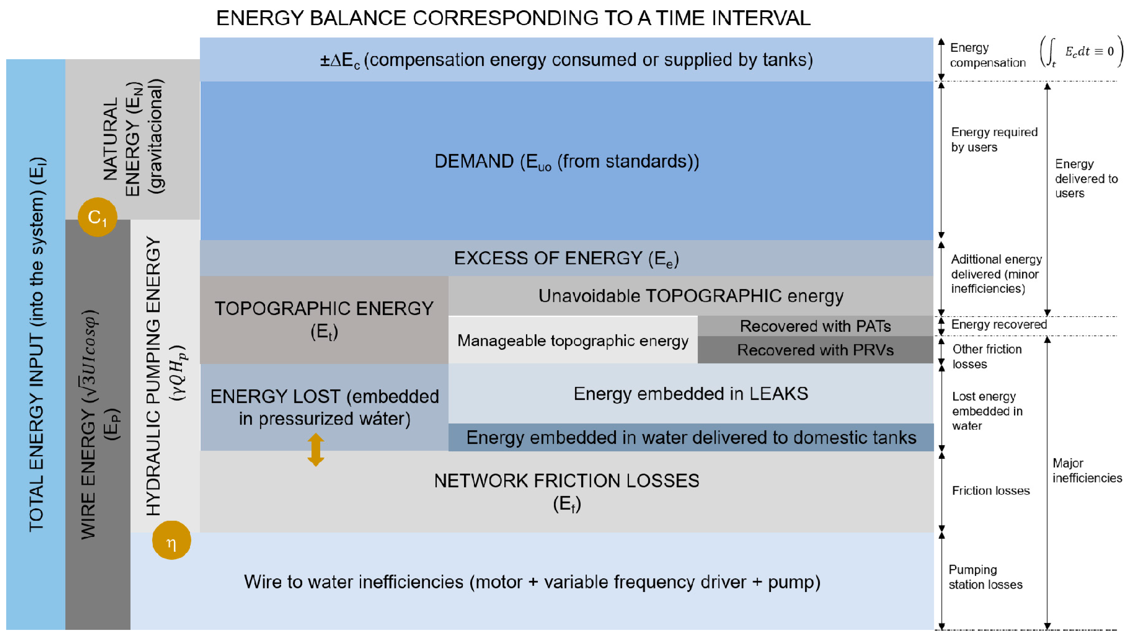
Figure 1 shows the global energy balance for a water network. As with any other balance, a certain timeframe must be provided. The context indicator C
1 [
5] specifies whether the total energy, E
I, injected into the system is natural (gravitational), E
N, or supplied by pumping (shaft), E
P. The values range from one, which indicates all energy is natural, to zero, in which all energy is derived from pumping. The natural energy, which is hydraulic in nature, is not affected by any reduction, whereas some of the shaft energy is lost due to inefficiencies in the pumping station. These inefficiencies are quantified by the global efficiency parameter η and are dependent on the operating point of the pumps and complementary devices, such as electric motors.
There are six possible destinations for the energy of the system. The concepts developed in previous works [
5,
6] are summarized as follows:
Compensation energy, ∆Ec. The energy involved in filling and emptying the compensation tanks. Energy is consumed as the tanks are filled and is released when they are emptied. Depending on the analysis interval, either a net consumption or supply of energy exists. When the energy balance is extended over a long-time period, for example, one year, the net result is zero.
Minimum energy required by users, Euo, is calculated from the user’s demand and the pressure set by the standards.
Excess energy, Ee, is energy that is over the minimum required by the users. This is avoidable energy.
Topographic energy, E
t. This is the energy required by the system as a result of the topography or the configuration. A portion of this energy is unavoidable unless the design is changed [
6]. The rest may be managed with pressure reducing valves (PRV) or with pumps as turbines (PAT).
Energy is embedded in leaks or is lost when water is depressurized in domestic tanks.
Energy dissipates in pipes through friction Ef; this energy is the focus of this paper.
To convert the qualitative balance (
Figure 1) to a quantitative balance requires an energy audit of a water system [
5]. In this analysis, different energies are coupled as leaks increase flows and, consequently, friction; accordingly, a modification of the operating point of pumps and their efficiency for a load condition means that each term of the balance can be independently calculated. As we focused on friction losses, once calculated, we needed to establish the final impact on the supplied energy by considering the pump efficiency, η.
In the global balance, natural energy is constant; therefore, any energy variation is a shaft energy variation. Clearly, as per the principle of energy conservation, the sum of all parts must coincide with the total supplied energy.
3. Optimum Hydraulic Gradient of a Static Network Flow
Given specific load conditions, J0 was calculated assuming that:
Current prices apply. Using current prices for pipelines that have been operating for decades might be considered incoherent. However, current optimum friction cannot depend on a network’s depreciation, and using current prices appears reasonable to achieve the pursued objective. Moreover, when it is time to renew the main (J0 will indicate the new diameter), it will be replaced with pipes at current prices.
Cost variations over time were not considered; firstly, because the optimal hydraulic gradient J0 is a value that depends on the current costs of both energy and materials and therefore changes over time, as do the costs, and must be updated. Secondly, the cost variations were not considered because its update helps to analyze the impact of new policies related to the increase in water and energy tariffs as well as the implementation of new environmental taxes.
The analysis can be performed at all times with current data as opposed to only completing it at the beginning stage, using design hypotheses.
Only the most significant economic factors, capital and energy costs that are both J-dependent, were considered. Other costs, such as investments in pumping stations, were not included because their dependence on J is minimally relevant. Other costs should only be included if the investment costs are strongly dependent on friction losses, such as pumping costs in a closed loop, and these costs account for a significant percentage of the overall investment.
The flow rates for the whole system were obtained from the network mathematical model.
Inefficiencies were coupled and consequently considered. Leaks were included in the model; therefore, flow rates were higher, as were investment and energy costs, as shown in Equations (4) and (16), respectively. The global efficiency ηg that accounts for losses at pumping stations is a multiplying factor of the dissipated energy, as shown in Equation (11).
The model does not consider local losses because they represent a low percentage of the total friction. If they were to be considered, the corresponding equivalent length would be added only in the energy term to the corresponding main length.
The friction factor was assumed to be constant and equal to the average value resulting for the entire system. This hypothesis could appear to be an over-simplification; as in a network, the friction factor is highly variable, although, in practice, it is not. An analysis of sensitivity proves this in the Sensitivity Analysis section.
3.1. Cost of Installed Pipes
The unit cost of mains per linear meter
Cp is calculated [
16] from:
where
a0(
p) is the constant pipe cost. This figure depends on the nominal pressure,
p, and on the pipe material. Both factors are assumed invariable in the analysed system. The value is calculated from commercial values.
D is the pipe diameter and
c is an exponent depending on the pipe material and the manufacturing process. The literature reports a wide range of possible values for
c. The widest range was considered, which covers all possible values, 1 ≤
c ≤ 2 [
17] to other slightly more restrictive ranges of 1 ≤
c ≤ 1.75 [
18]. In a later paper, Swamee et al. [
19] proposed the lowest value reported in the literature,
c = 0.866, which is valid for smaller diameter pipes. In each case, the exponent that best fits the catalogue prices should be adopted. Other documented values include 1.51 [
20] and 1.24 [
21]
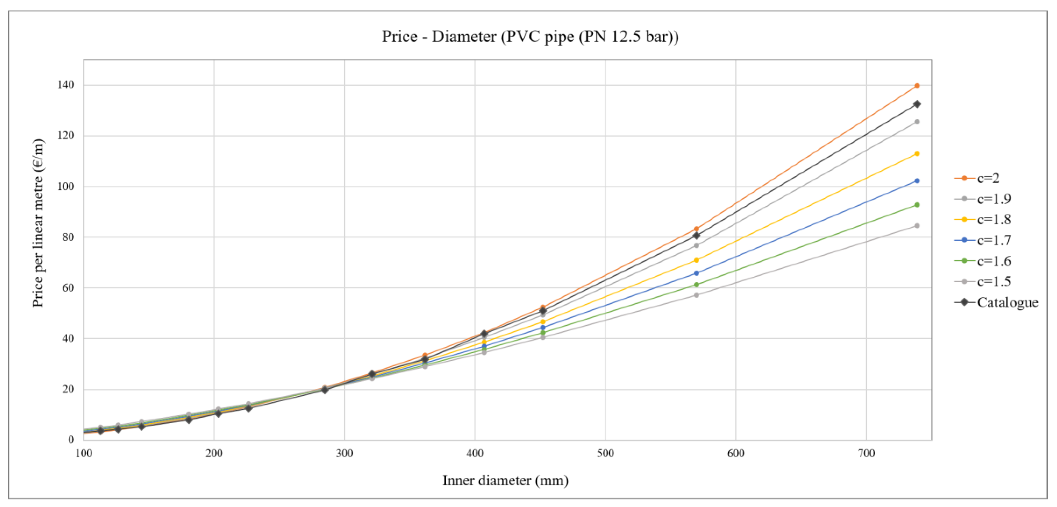
Both c and a0(p) were determined from the price catalogue. In the two examples provided in this paper (PVC and PE materials with nominal pressures of 6 and 10 bars, respectively), the final value for both cases was c = 2. Nevertheless, for ductile cast pipes with a nominal pressure between 30 and 64 bars and 32 and 85 bars, depending on diameter, the c values that best follow the prices trend were 1.6 and 1.2, similar to previously documented figures.
To finish, we must consider that Equation (1) only models the pipe cost. Transport, installation, restoring affected utility services, and other factors must also be included. The catalogue of additional costs is large [
22]. All additional costs must be included in the installation factor
Fi, which is sensitive to local costs and to the location where the pipe will be installed (urban or peripheral) as well as to its use (irrigation or urban). In short, the final price cost,
Cpf, of the installed pipeline is:
Practice shows that installation factors, Fi, range from 1.5 (irrigation use) to 3.5 in city center urban water networks. Therefore, each network requires its own individual analysis.
3.2. Annual Cost of the Network as a Function of the Hydraulic Gradient
The Darcy-Weisbach equation relates the hydraulic gradient
J (head loss
hf per length
L) with the flow rate
q, as follows:
where
f is the friction factor.
The combination of Equations (1) and (2) provides the pipeline cost as a function of the flow rate and the hydraulic gradient, leading to:
where
kp(
f,
p), is the pipe cost constant, equal to:
Notably, 0.0826 is a dimensional constant, only valid in the SI system framework. Therefore, appropriate units for q (m3/s) and D (m) must be used.
In consideration of the flow rate of each pipe
i of the system
qi, and a generic hydraulic gradient
J, the total cost (in today’s values) of the whole network
CN, is:
If a cost factor of the network,
λN, is defined as the product of the cost constant
kp and
, we obtain:
Assuming an average life span
n (years) for the pipes, the annual network cost is:
This cost depends on the network cost factor λN, the average pipe life span n, and the hydraulic energy grade line J.
3.3. Annual Energy Cost Dissipated Through Friction
In a static flow network, the final annual (yearly) energy
Efy needed to overcome friction losses in pipes is:
where γ is the water specific weight, and
h is the number of hours that the network operates annually. Regardless, the total energy consumed must include pumping inefficiencies. If
ηg represents the global pumping station performance (annual average value), the annual dissipated energy will be:
with all the variables expressed in SI units, except γ at 9.81 kN/m
3 and
h in hours/year,
Efyg results in kWh/year.
When a fraction of the supplied energy is natural, the energy savings represent an opportunity to reduce the pumping energy, which is the most expensive factor, while making full use of the available natural energy. Consequently, Equation (11) is valid as long as 1 – C1 > I3, where I3 is the ratio between Ef (energy dissipated in pipes through friction) and EI (total energy injected).
For an average energy price,
(€/kWh), the annual energy cost is:
where
e is the energy cost factor that depends on the network transport activity per unit of time,
. This concept is similar to the one used to measure the efficiency of any transport activity in tkm units [
23]. In summary, this energy factor
e is:
Therefore, the annual cost function to minimize the sum of both costs in Equations (8) and (11) is:
We must recall that Equation (13) provides the total costs (capital and energy), which are linked to friction losses. Other energy losses, such as the embedded energy in leaks, do not have a direct relationship with the network size and are therefore not included in this cost equation.
From Equation (13), the optimum hydraulic gradient is derived:
where
fp is, through
c and
n, a pipe dependent parameter. In short:
The optimum average hydraulic gradient for the network is:
Three parameters: fp, pipe dependent from Equation (15); λN, network cost-dependent from Equation (7); and e, energy cost dependent from Equation (12) prove that J0 is a parameter that also depends on the system and working conditions.
4. Refining the ELF Calculation Model
Equation (16) is traceable and therefore permits the substitution of the simplest hypotheses with other, more complex ones. Although they are presented separately, the hypotheses can be later combined. The potential improvements are described and their impacts on Equation (16) are analysed, including: (1) networks with different materials and pressures; (2) the energy supplied to the system as a combination of natural and shaft energy; (3) energy costs calculated from real rates and with environmental taxes; and (4) a network with dynamic behavior.
4.1. Networks with Different Materials and Nominal Pressures
Calculating the ELF requires modelling the price of pipes in accordance with a diameter that is sensitive to the type of material and the nominal pressure. Equation (16), which demonstrates the base of the optimum gradient
J0, assumes material and pressure uniformity in the network. If this is not the case, the system has to be divided into as many sectors (
k denotes the sub-system) as the materials present, finding the function to optimize each one as follows:
This expression clearly proves that capital costs are sensitive to the materials; however, energy costs are not. Equation (17) provides the optimum hydraulic gradient for each sub-system.
In old urban networks, finding pipes of different materials is normal. Over time, many older, once commonly used materials have been banned (e.g., asbestos cement) or abandoned, whereas new materials have been incorporated (e.g., HDPE). Managers are now likely to install the same material for the same conditions; however, in old networks, with different diameter pipes and conditions, situations in which pipes are of a single material for the whole network are almost non-existent.
4.2. The Energy Supplied to the System is a Combination of Natural and Shaft Energy
In previous papers [
5], some indicators to qualify the network behavior in terms of energy have been defined. In this subsection, two of indicators are of interest:
C1 (previously discussed) and
I3 (the ratio between E
f and E
I). This second indicator assesses the weighting of friction losses.
Consequently, if the shaft energy exceeds the friction inefficiencies (i.e., if 1 − C1 > I3), a friction reduction has a direct effect on economic savings because it supposes a reduction in the energy consumed in pumps. This, predictably, is the most common scenario.
When 1 − C1 > I3, the energy saved by the decrease of friction is not transferred directly to the energy bill (or only a part). In this case, from an economic point of view, the price of energy should be affected by a factor that compares the savings that have an impact on the pumped energy versus the total energy savings. This approach should be modified if the natural energy saved is recoverable through turbines.
4.3. Energy Costs Calculated from Real Rates with Environmental Taxes
In the previous model, a simplified average energy cost (€/kWh) was used. However, an electricity bill is somewhat more complex. In general, an electricity bill includes two items: the contracted power (kW) and the energy consumed (kWh). As part of a bill, unit prices can change over time, both throughout the day and depending on the month of the year. Significant penalties are incurred when the demanded power exceeds the contracted power. Finally, as a saving incentive, environmental charges can be included as part of an electricity bill.
Adjusting the cost of energy to reality is easy to implement; it only requires the breakdown of Equation (12) into the two terms included in the electricity bill: power and energy. The former is within the invoicing period (usually one month) and a fixed cost. As a result, the balance must be extended to the same time period.
In short, where
pep, the power cost (in €/kW and month)
pew, the energy cost (in €/kWh), and
hm the monthly hours of operation, the bill
Cem for that period leads to:
From which, we obtain the average energy monthly cost,
:
As energy tariffs vary throughout the year, pem is monthly dependent, which must be considered when extending this average monthly cost to a year. In any case, a similar procedure should be followed. The average yearly cost is calculated by dividing the yearly energy cost (Cey) by the total energy (kWh) consumed throughout the year (). On the basis of tariff structures and the economic balances, the average energy prices for short, medium, or long periods of hours, months, and years, respectively, were calculated. Notably, as the excess of required power over the contracted value can be avoided, this additional cost was not included.
Greenhouse gas emissions charges
pet, proportional to energy consumption, can be added to the energy cost. In this environmental context, a comparison of the sustainability of pipeline water transport with conventional means of transportation is important, a simple exercise using MJ/tkm [
23] as transport intensity unit
It instead of the traditional kWh/m
3. The friction energy resulting from transport, as the one required by users does not depend on transport, needs to be considered in MJ; it must then be referred to the displaced load (tkm). In short,
It is the quotient between the work required to overcome friction and the load factor, both per unit of time, leading to:
where
It, as works quotient, is dimensionless. Nevertheless, this indicator is singular because energies are in different unit systems. In the numerator of Equation (21), the specific weight of water is expressed in MN/m
3 (γ = 9.81 × 10
–3 MN/m
3), whereas the denominator is in t/m
3 (γ = 1 t/m
3), leading to:
For a
J value of 1.5 m/km and a pumping efficiency of 75%, the pipe transport intensity is 0.02 MJ/tkm. In comparison [
23] to other means of transportation (trucks 3.5 MJ/tkm, trains 0.3 MJ/tkm, and large ships 0.20 MJ/tkm), we conclude that this transport is by far the most sustainable.
5. ELF Calculation in a Dynamic Network
Equation (18) shows the optimum hydraulic gradient of a static network flow. This is the case for many irrigation networks (Example 1) programmed in similar shifts, which are as close as possible to the optimum conditions. However, in an irrigation network which has been scheduled to function on demand or in urban networks with time-varying patterns of demand, flows are not constant. The network’s behavior was simulated with hourly intervals with a quasi-static flow network model. For each hourly demand pattern, an optimum hydraulic gradient exists. However, as the gradient of every system is unique, determining which is best from among those 24 hourly optimum gradients is necessary or, if possible, other values close to any of the optimum gradients.
To determine this, a similar process to the one performed previously was followed, except with hourly intervals. For simplicity, we assumed that the hourly pattern demand was constant throughout the year. In this case, the cost calculation interval refers to the generic hour interval
j, adopted for this period. In a network operating uninterruptedly, the capital annual impact referring to an annual hourly period in Equation (12) is:
where
λNj, the network hourly cost factor, depends on the hourly flow rate
qij through the equation:
If the system does not work continuously, such as during rain storms, when irrigation networks are not in use, in developing countries, or in some urban networks, the investment must refer to the operating time. There is no amortization if the system is stopped. Nevertheless, the energy cost, which is intrinsically linked to the operating hours, is automatically adapted to the working hours in its energy term (not totally the less relevant power term, not included in this formulation, is time independent).
The annual energy cost of an hourly period from Equation (15) is:
where
hj is the annual number of hours that the system operates in the interval period
j, with
and
being the average energy price and global pumping performance in that period, respectively.
The hourly energy cost factor is:
In conclusion, for an hourly period
j, the annual cost function to be minimized is the sum of Equations (23) and (25):
which provides an optimum hourly hydraulic gradient equal to:
and similar to Equation (16). However, in this case, the cost parameters are variable with time, whereas the pipe dependent parameter
fp in Equation (15) remains constant.
The final step of the process, not needed in the static case, is to identify which of those 24-h gradients
J0j is the optimum
J0. Notably, once a
J0 for a given time has been adopted, the costs for the remaining periods depend on the selected gradient. The total cost for each hourly interval
J0j must be calculated using the equation:
Twenty-four values of optimal hydraulic gradient , with 24 different static conditions, one for each j time interval, were calculated. The total cost of the network was calculated assuming the same gradient for all different operating conditions. In this way, 24 total costs of the network were obtained, one for each different gradient, choosing the optimal that supposes a minimum total cost of each .
Because this is a potentially continuous function, the optimum may be provided by an adjacent value to one of the discrete 24 values. In this case, one of the discrete values was extremely close to the minimum; hence, we used this value without further calculations.
By plotting the corresponding curve with J0j and costs as the axes from among the 24 possibilities, a minimum value was found. The figure shows the absolute or relative characteristic of the selected minimum value. In very singular cases, such as firewater networks with practically zero energy costs, as J0 increases, the required investment and, accordingly, the capital costs in the absence of OPEX decreased. In this case, pumping costs, which are dependent on J, and other criteria, such as a maximum value for the velocity, should be considered. Otherwise, the optimum would not exist (J0 →∞).
6. Case Studies
To show the applicability of the model presented in this paper, two real case studies, static and dynamic, were analysed.
6.1. Case 1: Static Flow Irrigation Network
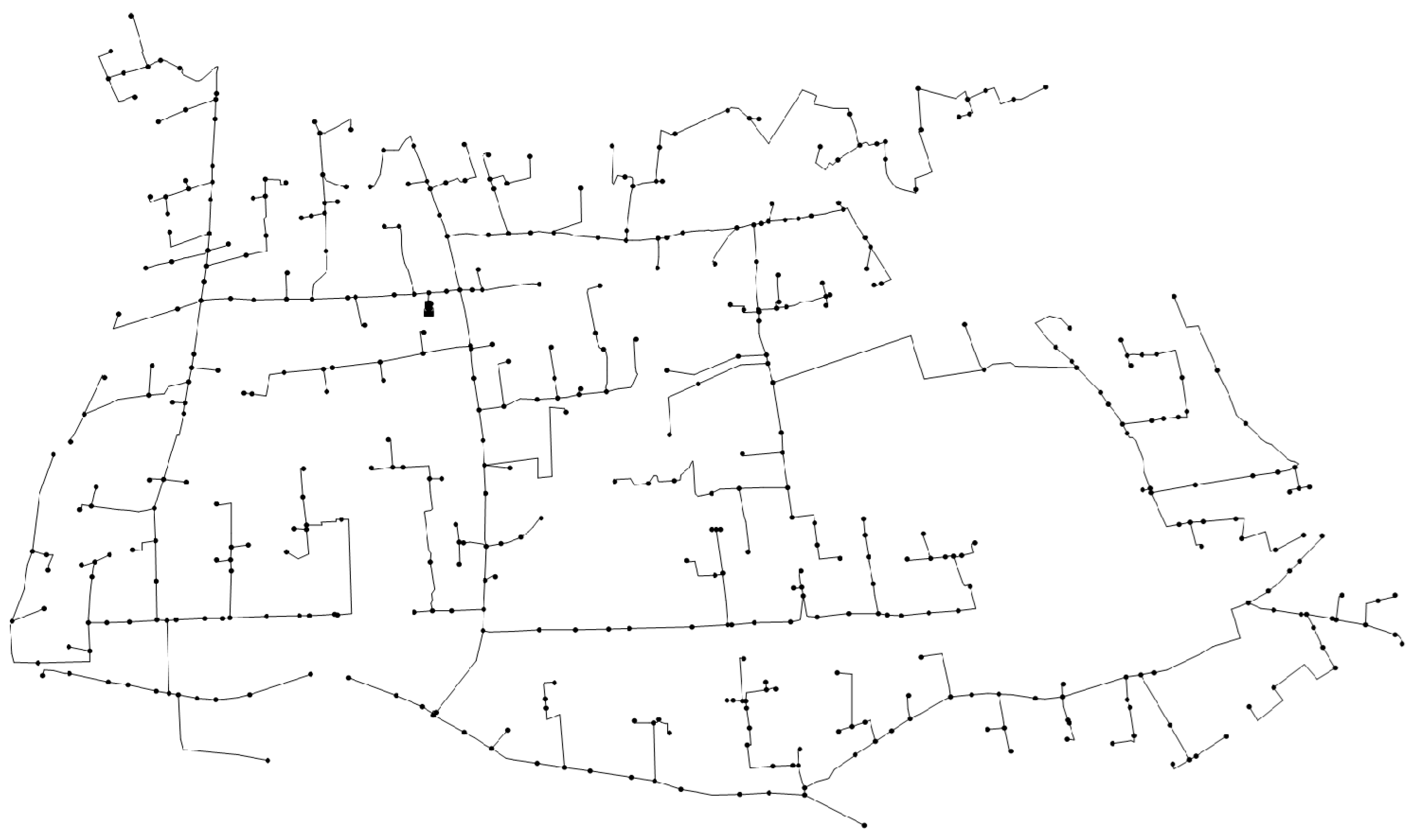
A tree irrigation network (
Figure 2) was analysed. Irrigation was scheduled for eight off-peak hours, from midnight to 8:00 a.m. Four similar shifts, each lasting for two hours, permitted static simulation because flow rates were practically constant except at the smaller end branches. The number of irrigation hours per year depended on annual rainfall. Basic parameters were as follows: total network length was 55.37 km, total flow was 672.30 L/s, operating hours were 1600 h/year, current diameter range was 63–800 mm (majority 200 mm), material was PVC, and network pressure was 22–63 mWc (average pressure 36 mWc).
6.1.1. Network Annual Capital Cost
On the basis of the PVC pipe price catalogue (PN12.5), the value of
a0(
p) was calculated and the exponent
c was adjusted. Results were
a0(
p) = 256.29 €/m·m
2 and
c = 2 (
Figure 3).
Complementary data included the average friction factor,
f = 0.014; installation factor,
Fi = 1.6; and pipe life span,
n = 50 years. The network cost parameter
λN was:
6.1.2. Network Annual Capital Cost
The average energy cost of this network with energy and power terms included is
= 0.12 €/kWh, constant for the eight off-peak hours. Efficiency of the pumping station was
ηg = 0.7. From these values, and taking into account the network load factor, the annual energy cost
e was:
The optimum hydraulic gradient was:
with an annual total cost equal to:
The contribution of the annual capital cost was 71.4%, whereas the annual cost of the required energy to dissipate the friction was 28.6%. The total energy bill was obviously higher because the aforementioned amount was only for dissipation through friction. If we compare J0 with the actual value , at 1.35 m/km, which was the average head loss weighted with flow and length for the entire pipe network, we can conclude that, for the actual operating conditions at current prices, the friction that occurred in the network was above the optimum value of friction. Therefore, the network was convenient to study from a cost-benefit point as well as the possibility to reduce friction losses in the network.
The context indicator C1 was 0.217 (i.e., 78.3% of the energy supplied to the system is shaft energy), whereas I3 was 0.044, meaning only 4.44% was friction loss. Therefore, shaft energy exceeded friction inefficiencies (clearly 1 − C1 > I3) and, therefore, energy costs were correctly estimated.
Finally, with an optimum hydraulic gradient of 1.75 m/km and an efficiency at the pumping station of 0.7, the optimum transport energy intensity It, from a strictly economic point of view, was 0.024 MJ/tkm.
6.2. Case 2: Dynamic Urban Network
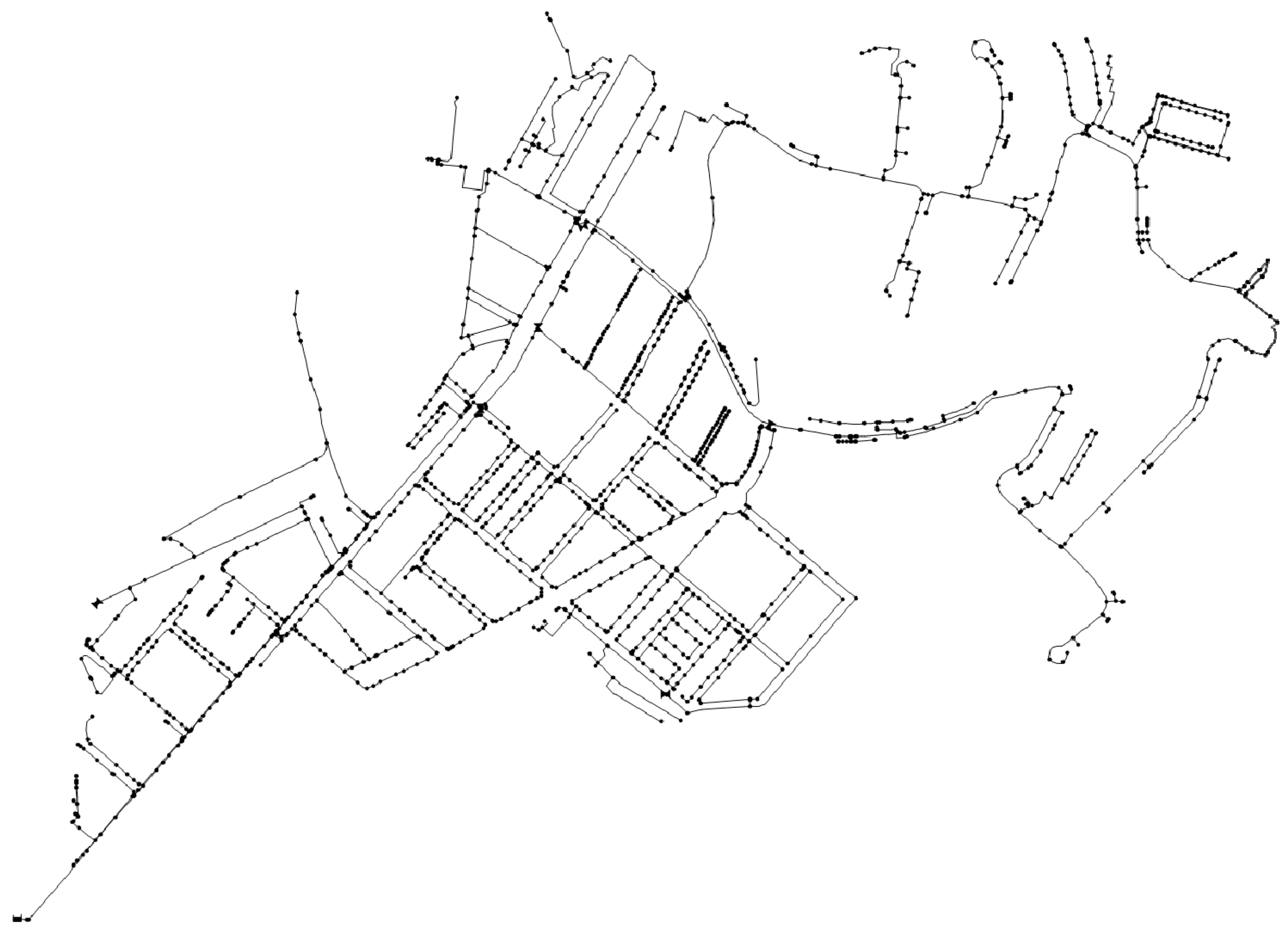
Case 2 represents a District Metering Area of a Spanish urban network (
Figure 4). Parameters included total network length: 27.23 km; supplied average flow: 59.59 L/s (21.93% of this flow corresponded to leakage); operating hours: 24 h/day (with the corresponding pattern demand); current diameter range: 32–400 mm (majority 80 mm); material: asbestos cement (52%), HDPE (40%), and Ductile cast pipes (8%); and average network pressure: 70 mWc.
Although the current pipe material in this network was predominantly asbestos cement, it was being replaced. Concurrently, as it is no longer manufactured, no catalogue prices were available. For this reason, we assumed that all the new pipe material was polyethylene. For HDPE (PN10), on the basis of the catalogue data, results were a0(p) = 583.38 €/m·m2 and c = 2. A mean friction factor f = 0.016 was assumed, whereas the installation factor (higher than in the previous urban network case) was Fi = 2.3. As a final point, the same pipe lifespan was adopted (n = 50 years).
A real Time of Use (ToU) tariff was applied and the prices included off peak time = 0.042930 €/kWh, shoulder time = 0.120514 €/kWh, and peak time = 0.187982 €/kWh, with power terms included in the preceding energy costs. The average global efficiency for the pumping station was 0.75, assumed constant for all time periods. For these values, the different
J0,j are outlined in
Table 1.
The total cost of G
Ty,j in Equation (33) was calculated assuming a constant value of
J0,j for the entire day but in consideration of both the daily demand pattern and, accordingly, the flow rate for each hour. Once the total cost for each value of
J0,j was calculated, the final solution
J0 was the one with the lowest cost. In this case,
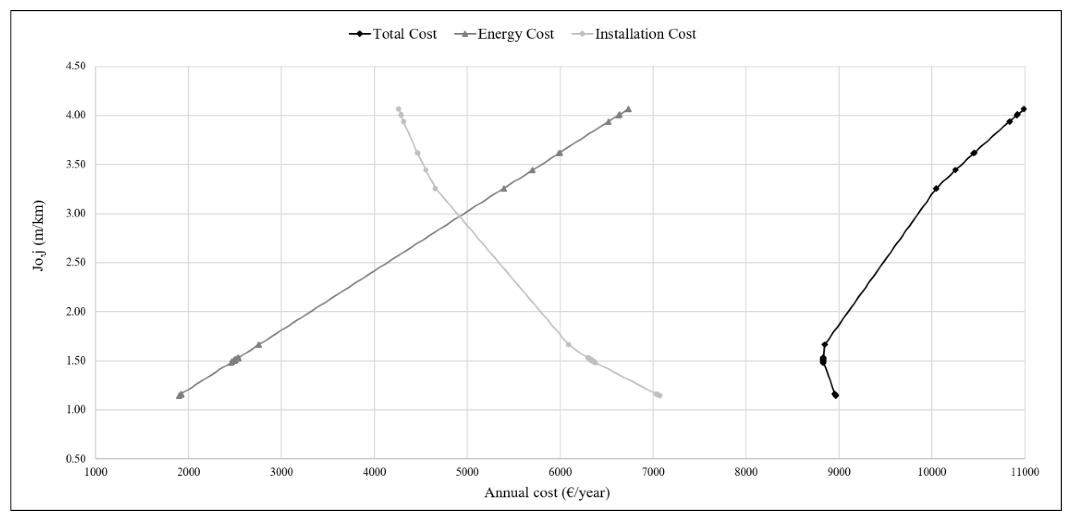
J0 was 1.65 m/km, which matches the optimum gradient calculated for 4:00 p.m., with a total annual cost of 6512 €, of which 72% was capital costs and 28% was energy costs.
Figure 5 shows the results for each time interval as well as the existence of a total minimum cost (optimum). In this case, the value almost coincided with that corresponding to
J0 = 1.65 m/km. Should the costs curve not show an absolute minimum value, an exploration of other
J values outside the interval defined by the hourly demand patterns would be necessary; in this case, from 1.242 to 4.081 m/km, but such values must always be within reasonable limits, for instance, from 0.5 to 6 m/km. Only in very rare cases, such as with very short operating times in a fire network, the minimum value will not be within the explored interval.
If this same system is analysed as a static flow network, with nodal demands equivalent to the daily average, the optimum hydraulic gradient would be 1.81 m/km, slightly higher than obtained in the dynamic simulation. Finally, the actual hydraulic gradient of the network, , weighted by the flow and the length of each pipe, was 0.8 m/km, which is a value lower than the optimum gradient of 1.65 m/km.
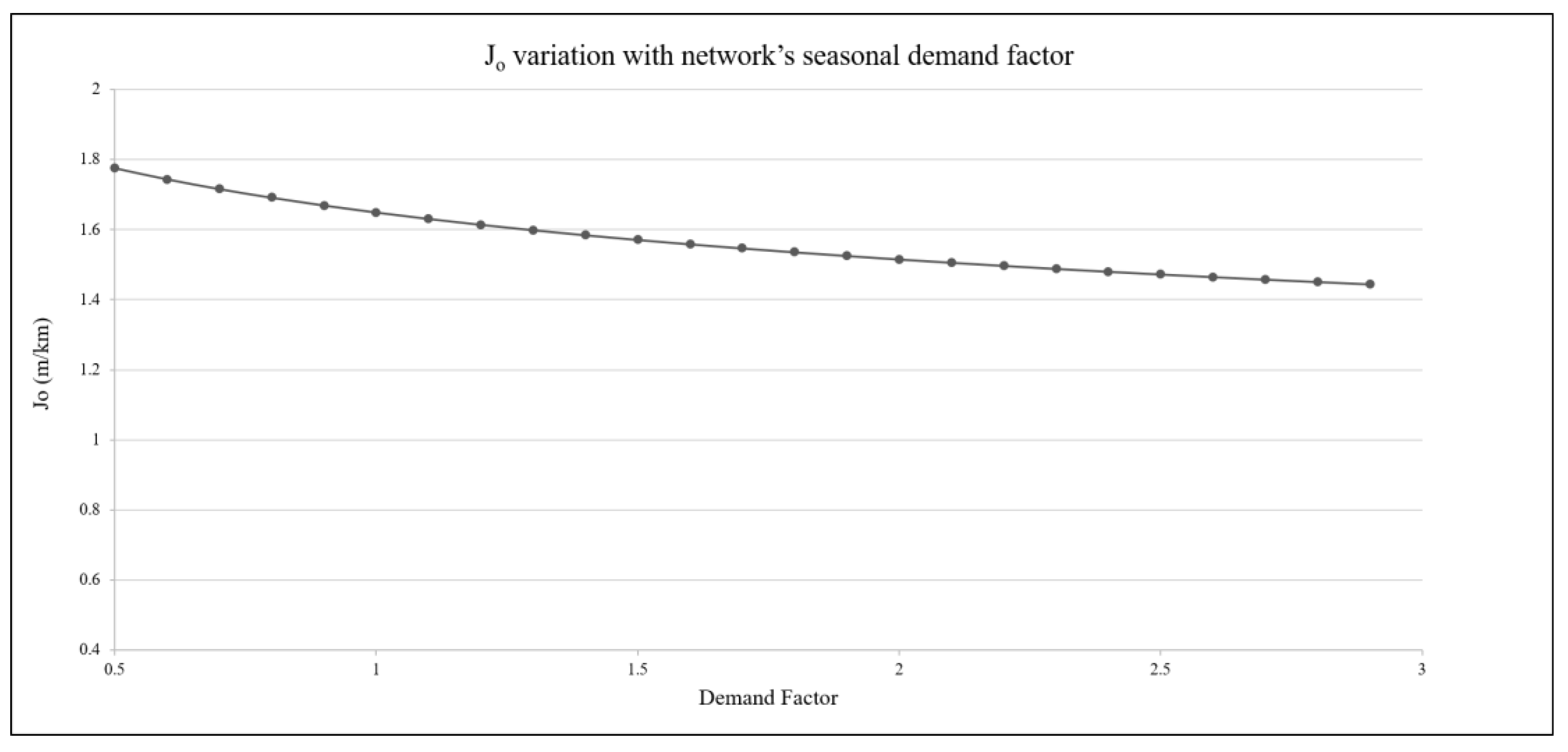
Finally, an exploration of the evolution of
J0 in systems with significant time flow variations is convenient, such as for cities with a high seasonality factor.
Figure 6 illustrates this evolution, showing the limited impact of these variations. Taking into account the same pattern but with different demand factors, from 0.5 to 2.9 m/km, the variation in
J0 was quite moderate, ranging from 1.77 to 1.44 m/km (
Figure 6). A variation that has little impact on
J0 led to a discrete set of solutions (diameters), and similar
J0 values will result in the same commercial diameter. Conversely, the impact of this short interval is, in practice, very low. As the range of commercial diameters is discontinuous, regardless of the
J value, the solution is the same. For example, in this case study, we obtained identical solutions (diameter = 400 mm) using the upper value (
J = 1.77 m/km, D = 376 mm), the lower value (
J = 1.44 m/km, D = 392 mm), or the optimum solution (
J0 = 1.65 m/km, D = 380 mm).
This low
J0 dynamic variability can be explained by Equation (20). Both the numerator λ
N and the denominator
e are sensitive to the circulating flows. However, whereas the exponent for the former is 2
c/5, which is 0.8 when
c is 2, the dissipated energy
e increases linearly with the flow. Therefore, as the denominator increases at a faster rate than the numerator, the final value of
J0 decreases (
Figure 6). However, because both exponents were similar, the result barely changed. Lower values of
c in the pipe cost function reduced the weight of the numerator, whereas the energy factor was maintained. This slightly diminished the value of
J0; however, the 2/5 multiplying factor mitigated this effect.
7. Sensitivity Analysis
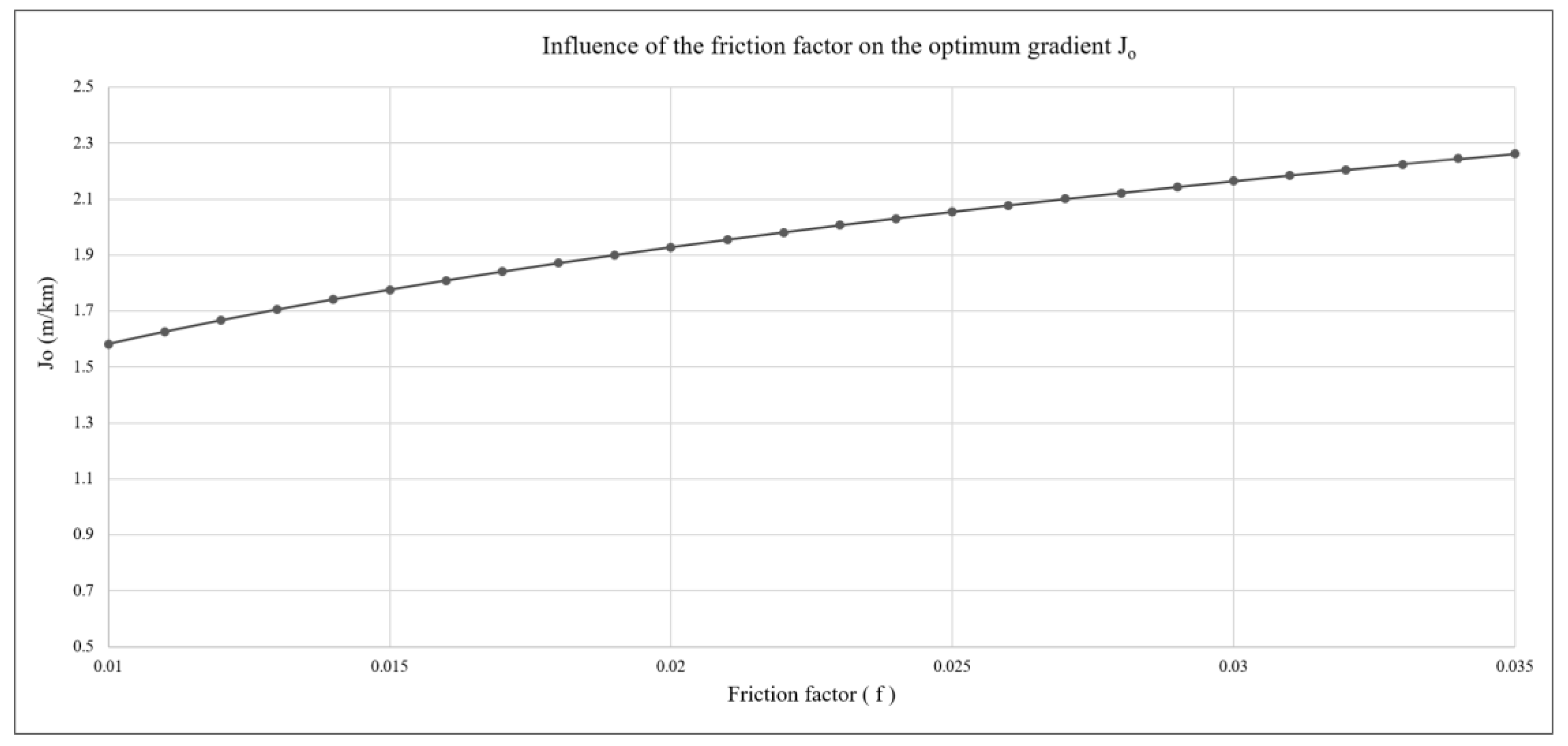
From the results obtained in the irrigation network, a sensitivity analysis was performed. Firstly, to validate one of the hypotheses that could appear weak, the impact of the constant friction factor
f was explored.
Figure 7 validates this hypothesis. Having calculated
J0 for different
f values from the lowest to the highest, as found in the network analysis, the plotted results show a quasi-flat curve. The selected
J0 (
f = 0.014) is the network weighted average.
Conversely, the value of
J0 was very sensitive to certain pipe cost parameters, such as the pipe lifespan
n (
Figure 8). By shortening the life of pipes, the capital costs became relevant and
J0 increased to mitigate this impact, whereas an increase in life expectancy produced the opposite effect. This behavior was not symmetrical. Although a 60% reduction (20 years) in the lifespan of a pipe increased the value of
J0 from 1.75 to 3.38 m/km, a similar extension in its life (60% or 80 years) had a reduced impact on the change of
J0 (1.75 to 1.25 m/km). The remaining parameters changed linearly.
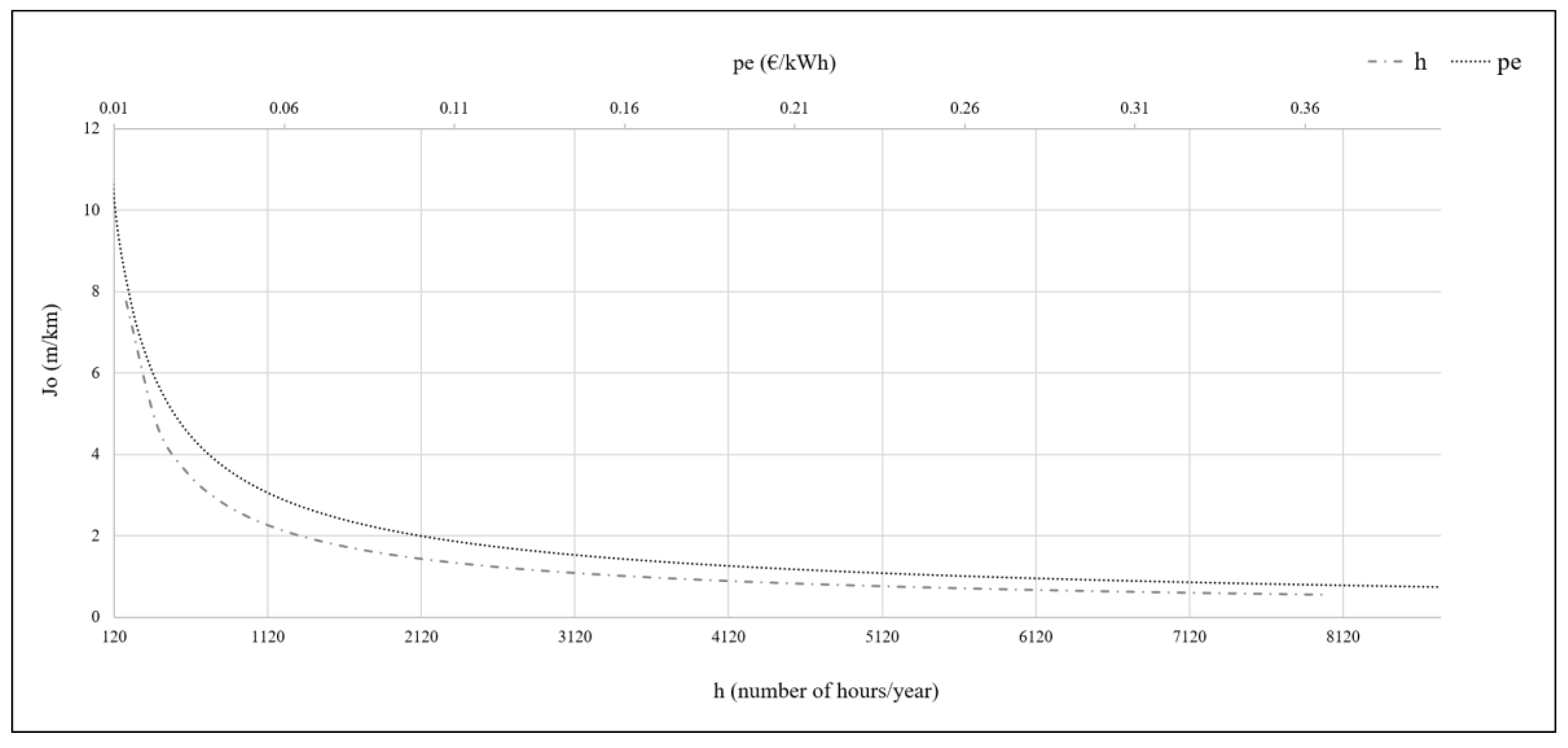
Figure 9 shows
J0 sensitivity to two key OPEX parameters: energy cost and operating hours of the system. A dramatic variation occurred when the system only operated a few hours per year. Fire water networks were the most extreme case, where h→0. In the second example, a similar influence of the energy cost in
J0 was found.
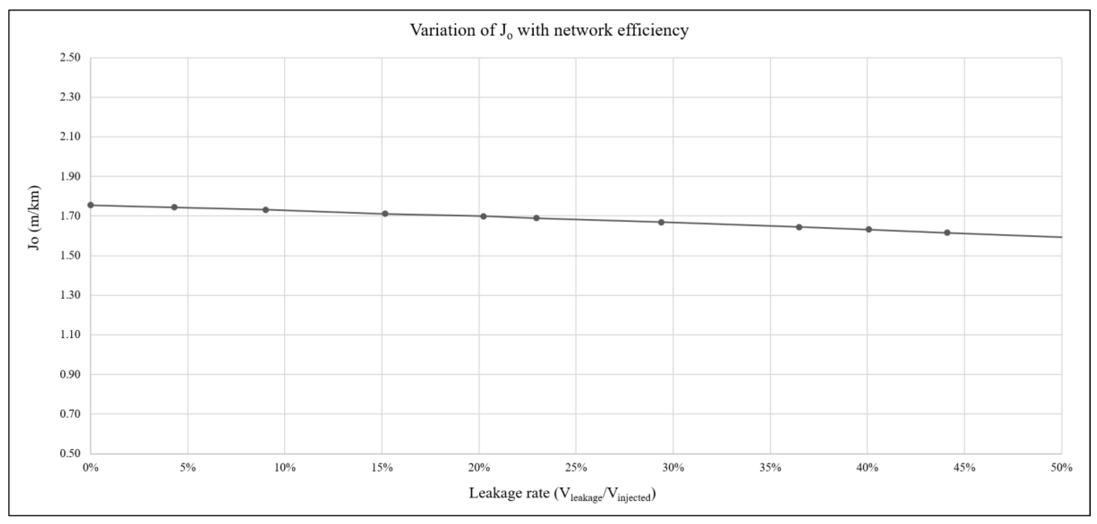
Finally, the sensitivity analyses for the inefficiencies are presented.
Figure 10 shows the variation in
J0 with leakage. The sensitivity was low; even when the flows were duplicated (50% efficiency), the optimum gradient barely changed (1.75–1.59 m/km). This was hardly surprising since, in the same system and with an identical framework,
J0 varied little with increased flows, as previously shown for the demand factor (
Figure 6).
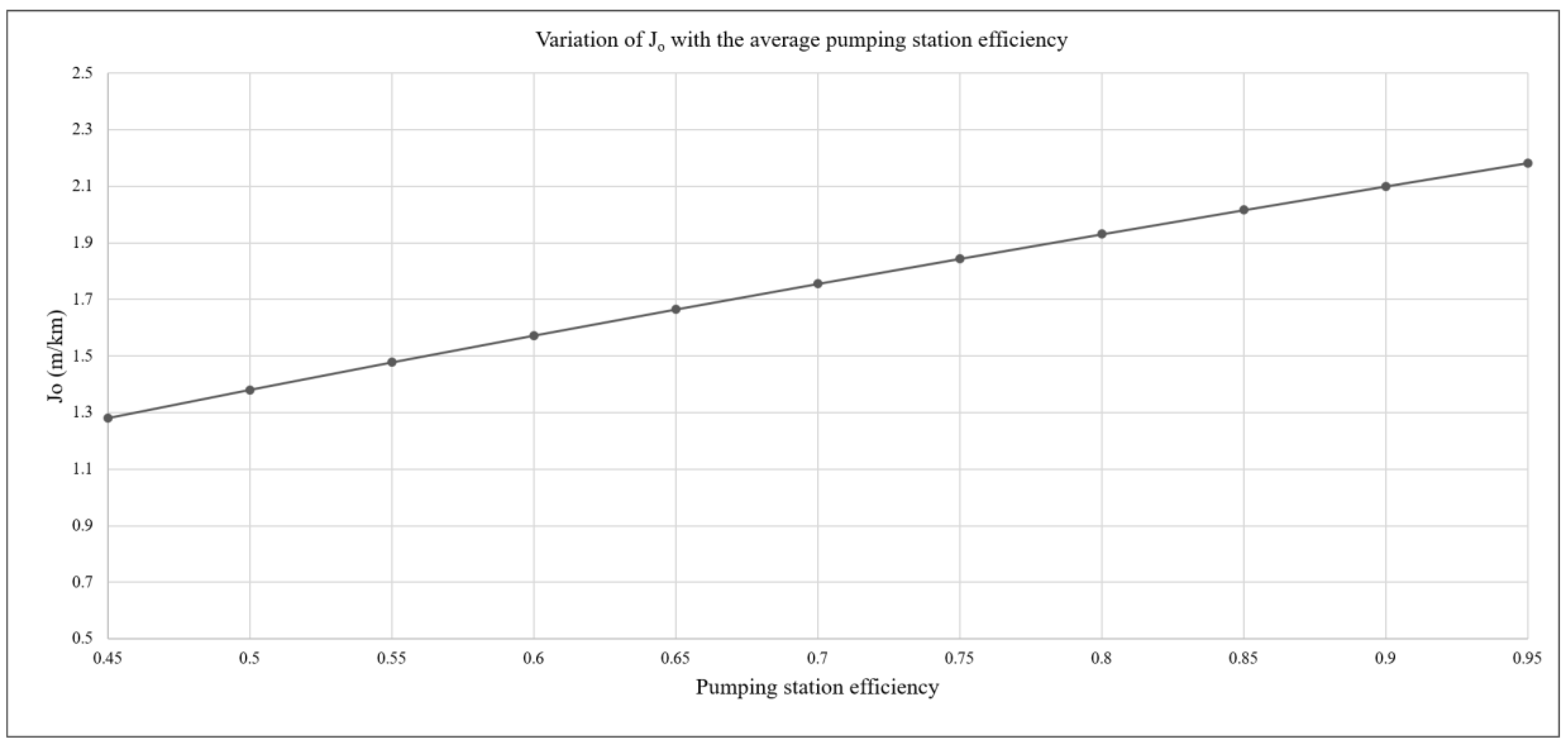
However, the influence of the average efficiency of the pumps was greater because only the denominator of Equation (16) had an impact. A diminishing efficiency yielded greater energy costs and a decrease in
J0 (
Figure 11).
A discussion of the potential error in the ELF value is relevant because the pumping station costs were not included in the CAPEX costs. Two factors provide the answer. The first is the impact of friction losses in the total head pump: if this value is moderate because the energy needs are led by service pressure requirements and elevation, the pumping station costs, even in consideration of their shorter life span of around 15 years, are practically friction independent and therefore do not influence J0. Secondly, if the cost of the pumping station is a small percentage of the total cost of the network, the effect is also minimal. Currently, in urban or irrigation networks, this may account for 5% of the total costs. Therefore, we conclude that including pumping costs in the CAPEX is not necessary. Perhaps this would not be the case with a closed industrial water circuit.
8. Results Analysis and Validation
The methodology to obtain J0 was based on the validity of the supporting hypotheses, on the quality of the mathematical model of the network, and on the consistency of the context parameters. The process to calculate J0 was deterministic; it did not rely on random factors or on forecasts.
The case studies were selected on the basis of two criteria: a search for complementarity and verification that all the required information was available. The irrigation network operated eight hours/day; however, it remained pressurized at all times to avoid air intrusion and bursts. Therefore, the relationship between
J0 and the hours of operation was obvious. In this example, as the network only operated during off-peak hours, the energy cost was constant. The second network corresponded to a District Metering Area, a subsystem of an urban network, which served a stable population. This example shows that
J0 was only slightly sensitive to dynamic changes. To demonstrate this, large flow variations were introduced through the demand factor (
Figure 6). In practice, this low variability had a limited impact (in practice, the solution was essentially the same) and the adopted
J0 corresponded to the average demand factor. The same effect was analysed in the irrigation network through the hydraulic network efficiency in this case (
Figure 10). In the end, we obtained identical conclusions.
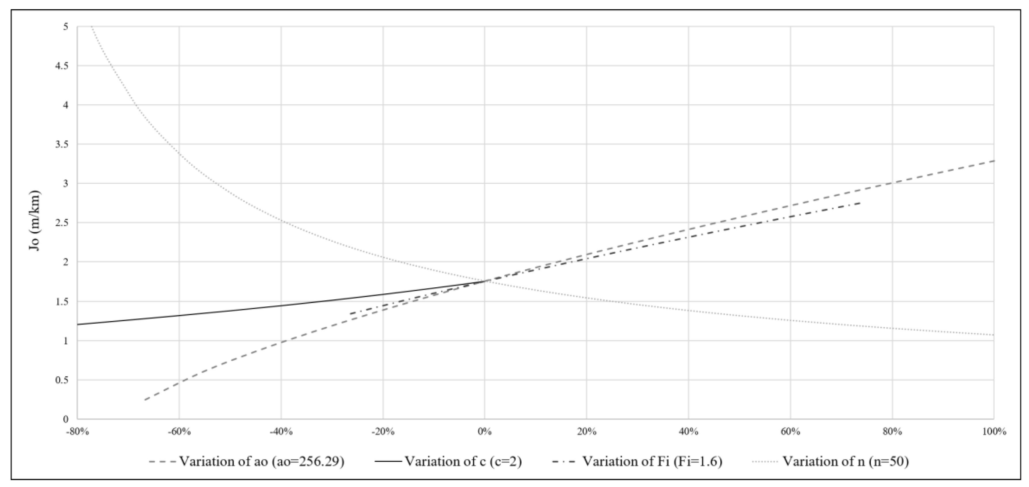
However,
J0 showed high sensitivity to both kinds of costs: first, to CAPEX, through the pipe cost constant value
a0, the diameter exponent in the cost variation equation exponent
c, the installation costs
Fi, and the average life,
n (
Figure 8); and, second, to OPEX, through the time of activity (hours of operation per year), the price of the energy (
Figure 9), and the tariff structure, and, to a lesser extent, the pumping efficiency (
Figure 11).
Table 1 highlights the influence of the electric tariff on the final value of
J0 and simultaneously proves that operational costs had a greater impact on the result than the dynamic behavior of the network. An initial analysis suggested, in an apparent contradiction with the above, that
J0 was quite sensitive to dynamic flow changes, as the range of 1.215 to 4.06 range was very wide. However, a deeper analysis showed that these values were greatly influenced by the hourly price of energy and were much less sensitive to the flow rates. This was evidenced during the period when the price of energy was lowest (0.042930 €/kWh), as the values of
J0 were surprisingly high, showing a much greater influence than that of the circulating flows.
In conclusion, the time and space aspects of J0 prevented any kind of comparison, even between similar networks. Results must be compared in consideration of the context of the system. Therefore, such a comparison makes sense within the same network (J0 vs. ). An analysis of a set of real networks would be interesting, assuming that all the information is available, and comparing J0 with in all networks. These differences would provide relevant information on how, in practice, context information affects the gap ( – J0) and when and where networks have or have not been well designed.
Although the developed procedure is valid for any kind of network, a further generalization was needed to include pumping station costs in the total capital cost function in very particular cases. With this in mind, this inclusion only makes sense when the pump selection is strongly influenced by the friction losses level. This is not an easy task. Pump costs are highly variable and, despite the proposal of some models in the technical literature [
19,
24], they are far from capable of reasonably reproducing actual price variability. A major cause for this is that pump costs depend on many factors, such as type of pump, materials, manufacturing, and efficiency. This is not the case with pipe costs, as they can be adjusted fairly well, given that they are more standardized products. Furthermore, these pump costs should be modelled with their dependence on
J, as we have done with the pipe cost in Equation (4). Fortunately, owing to aforementioned reasons, this is not necessary in urban and irrigation networks, such as the ones considered in this paper.
9. Conclusions
A new metric to assess the energy efficiency of a pressurized water network from the point of view of friction losses was developed. We compared the average optimum hydraulic gradient J0 and the current value, , to determine if friction losses are economically acceptable in a given network and context. This metric plays a similar role to the well-established economic level of leakage (ELL). Both are economic benchmarks of network inefficiencies and both are highly dependent on context parameters and service conditions. In addition, J0 is a reliable substitute for the guide values provided in the literature for the hydraulic gradient J and can update the pipe replacement criteria.
Once J0 is well established, available metrics can independently assess the three main energy inefficiencies, friction, leaks, and pumping, in a water network. Although these inefficiencies are dependent on each other, they can be determined independently for a given load condition. The overall energy efficiency of a system is a combination of these three partial efficiencies. The final result will only be maximized if the existing interdependence is adequately addressed. For instance, it is illogical that the most efficient point of working pumps corresponds to a leaky system with excessive friction losses. This paper has clarified this issue and is therefore the starting point for further global assessment.


