Hydrological Modeling in Data-Scarce Catchments: The Kilombero Floodplain in Tanzania

 , , , and
Abstract
:1. Introduction
- (i)
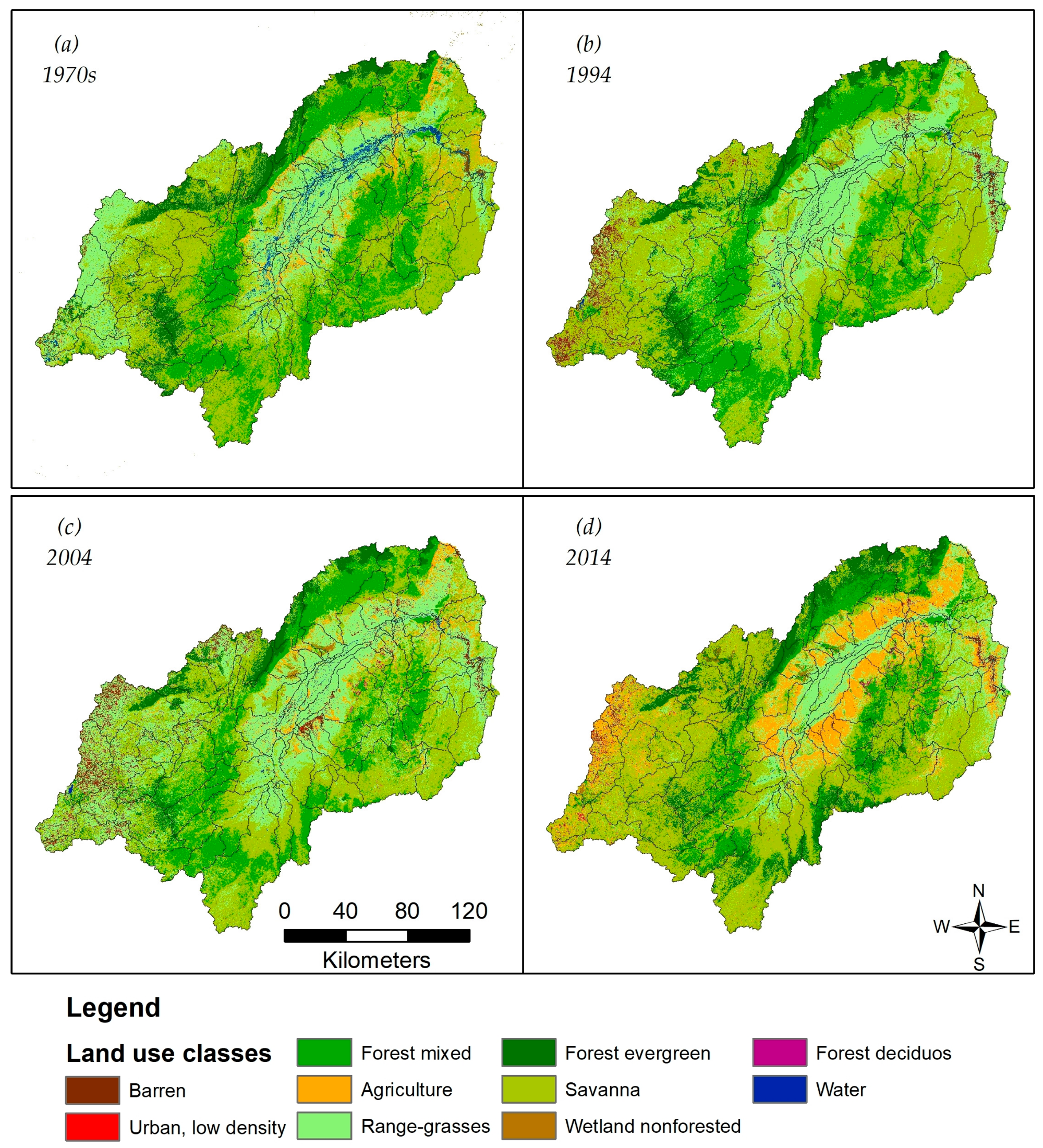
- Assessing LULCC in the Kilombero Catchment since the 1970s;
- (ii)
- Setting up a distributed hydrological model suitable to simulate impacts of LULCC;
- (iii)
- Analyzing the impacts of LULCC on water balance components in the catchment.
2. Materials and Methods
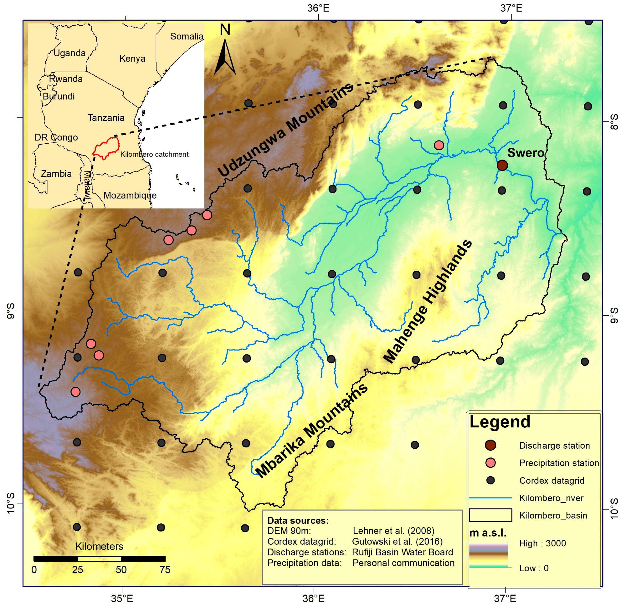
2.1. Study Site
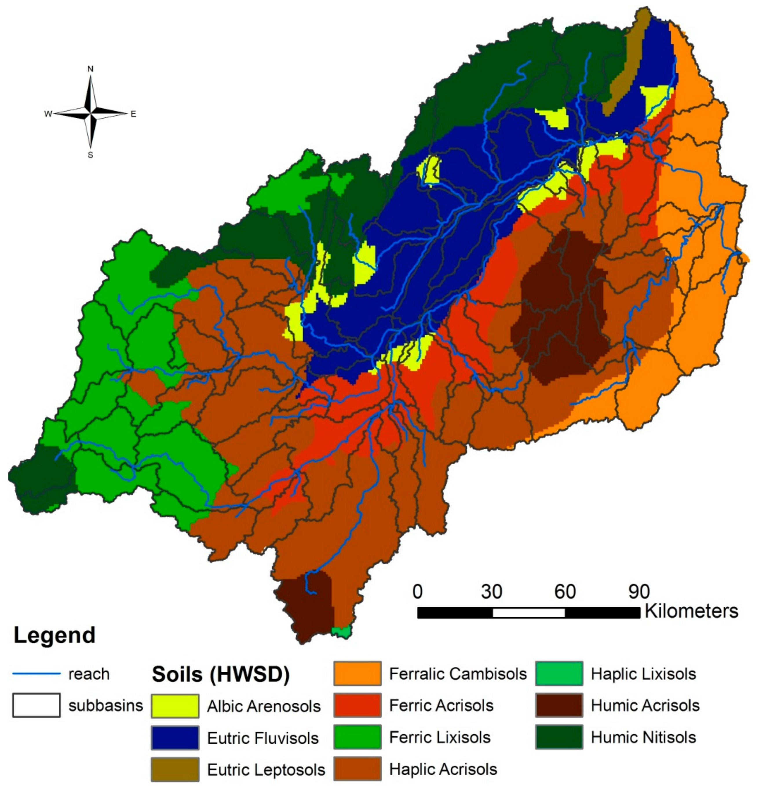
2.2. Input Data
2.3. Model Description
2.4. Model Setup and Evaluation
3. Results
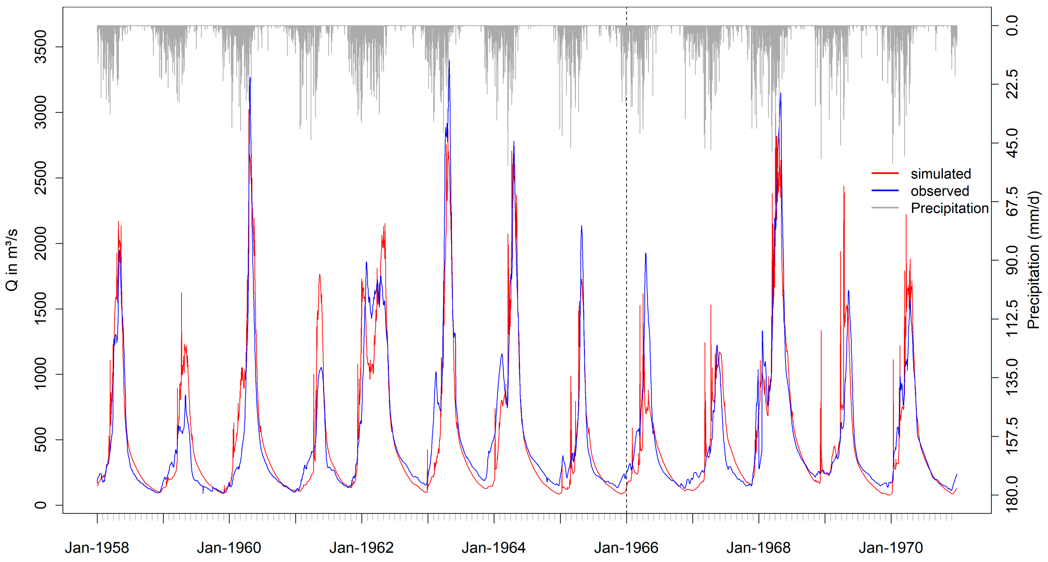
3.1. Model Calibration and Validation
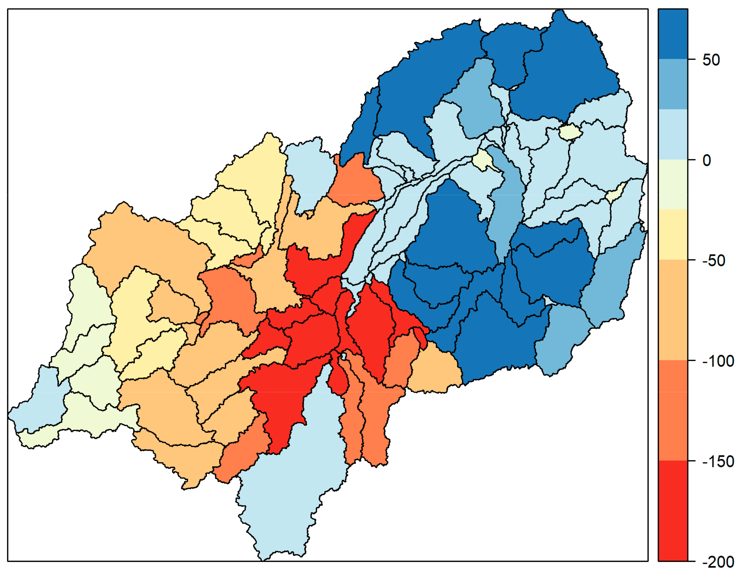
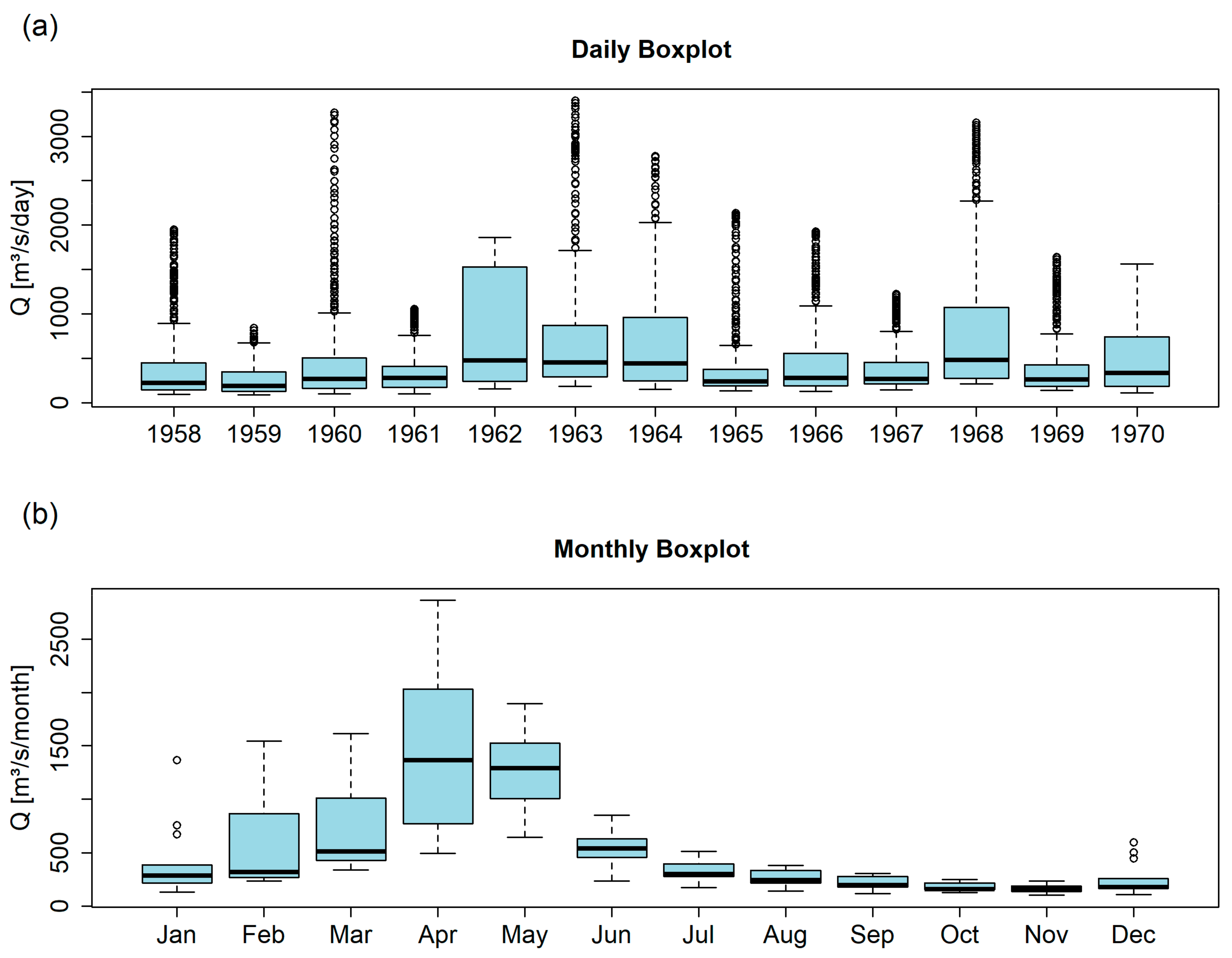
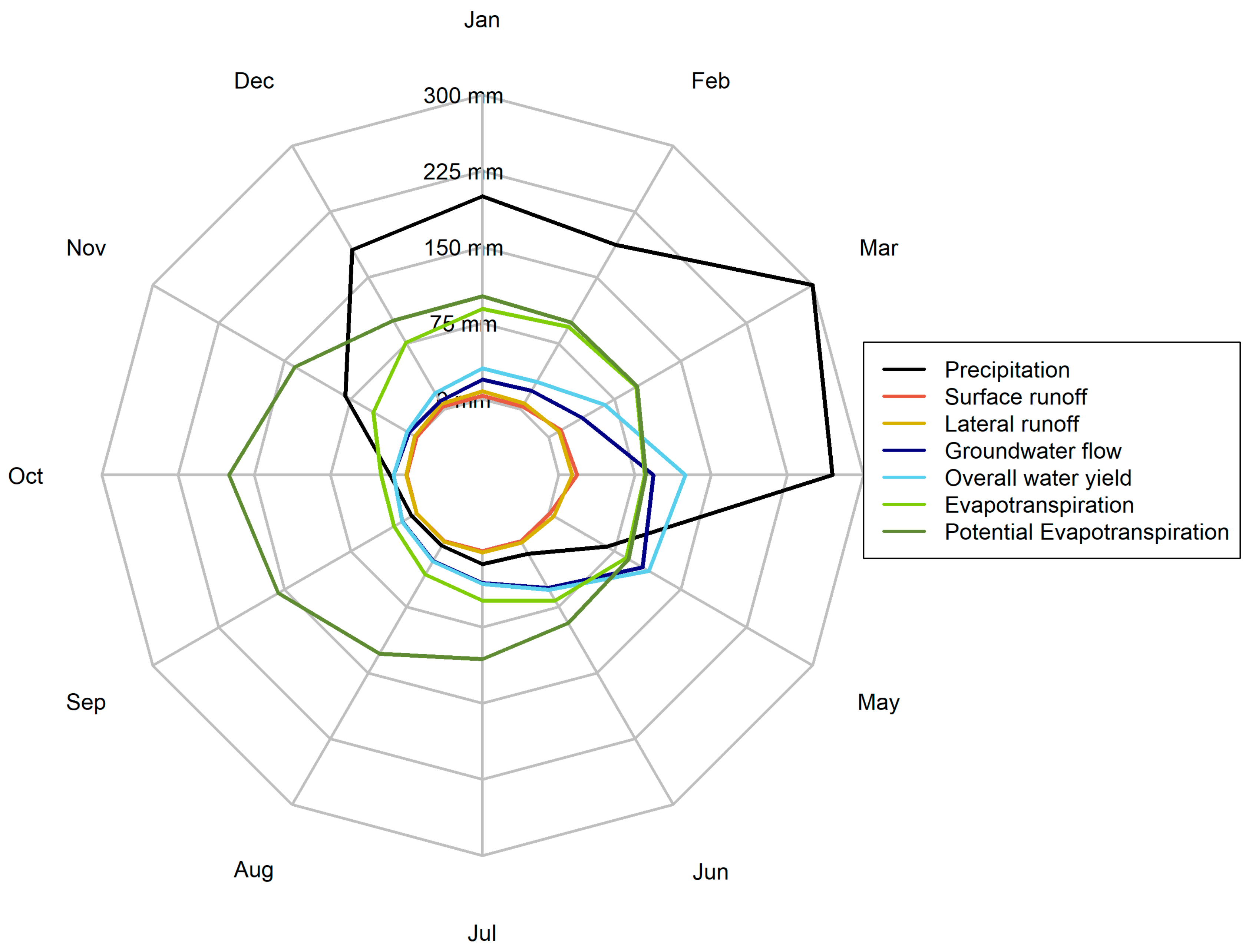
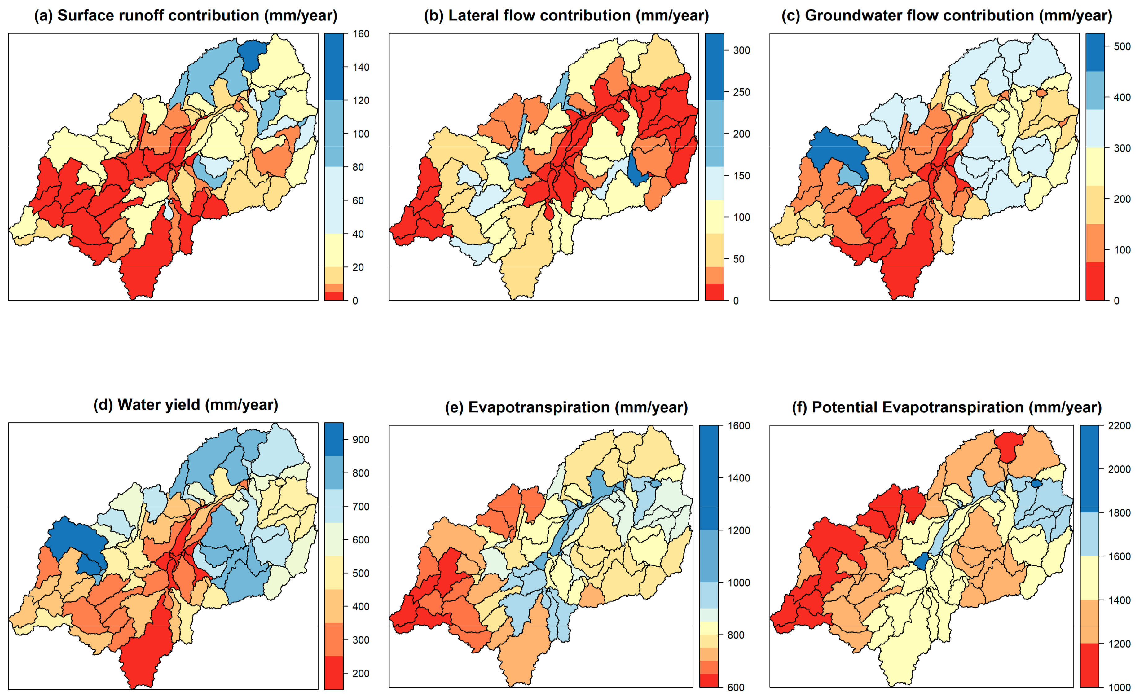
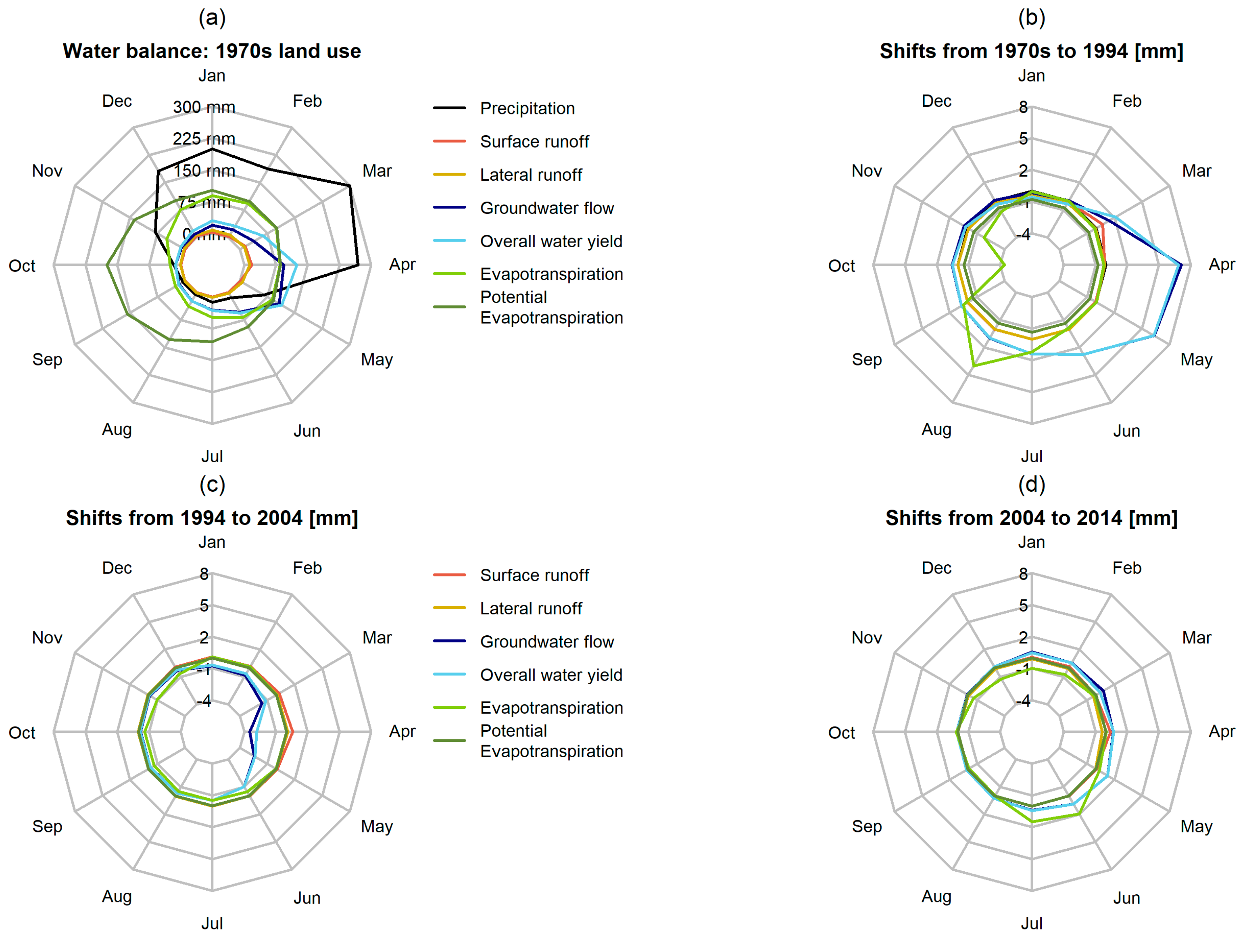
3.2. Spatio-Temporal Analysis
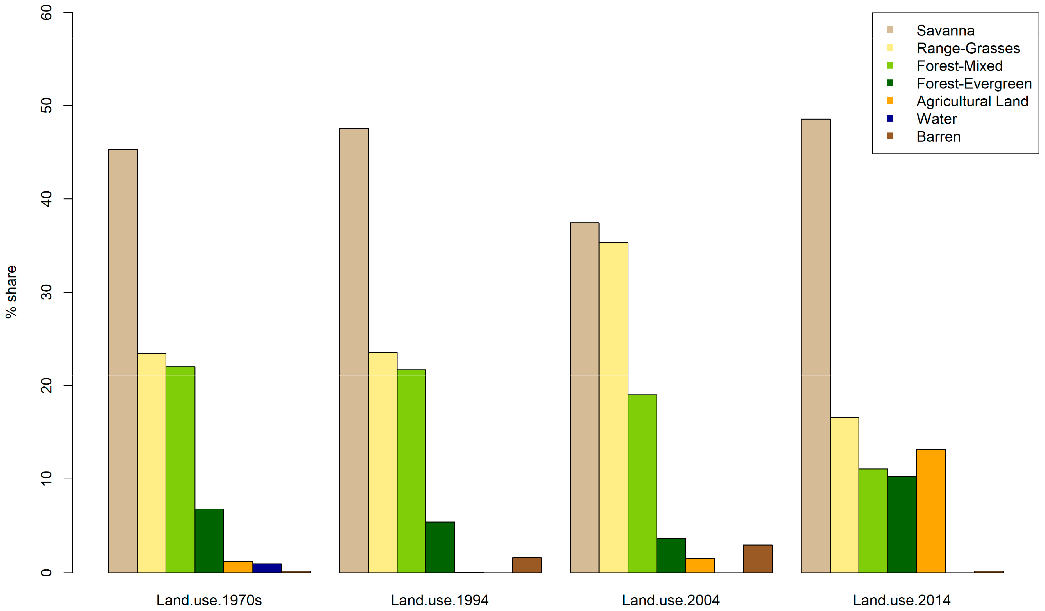
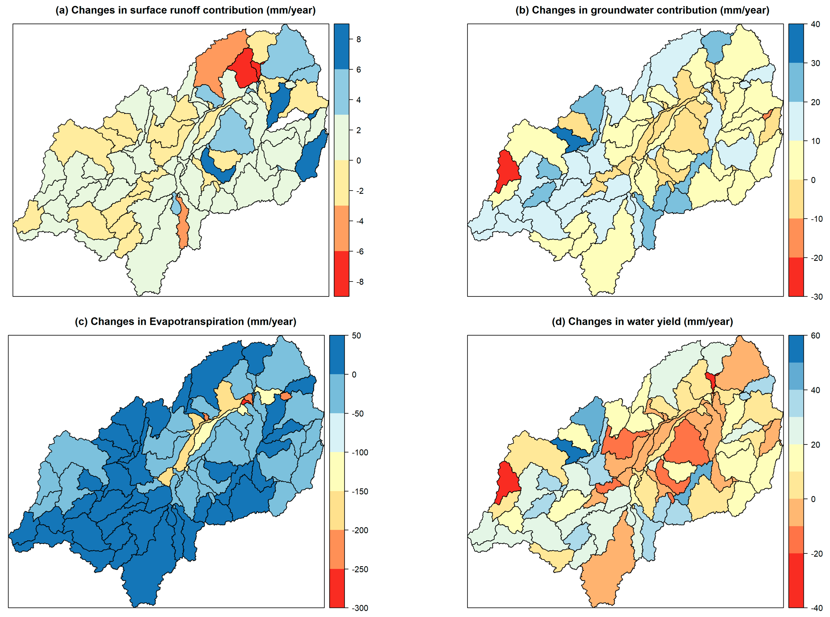
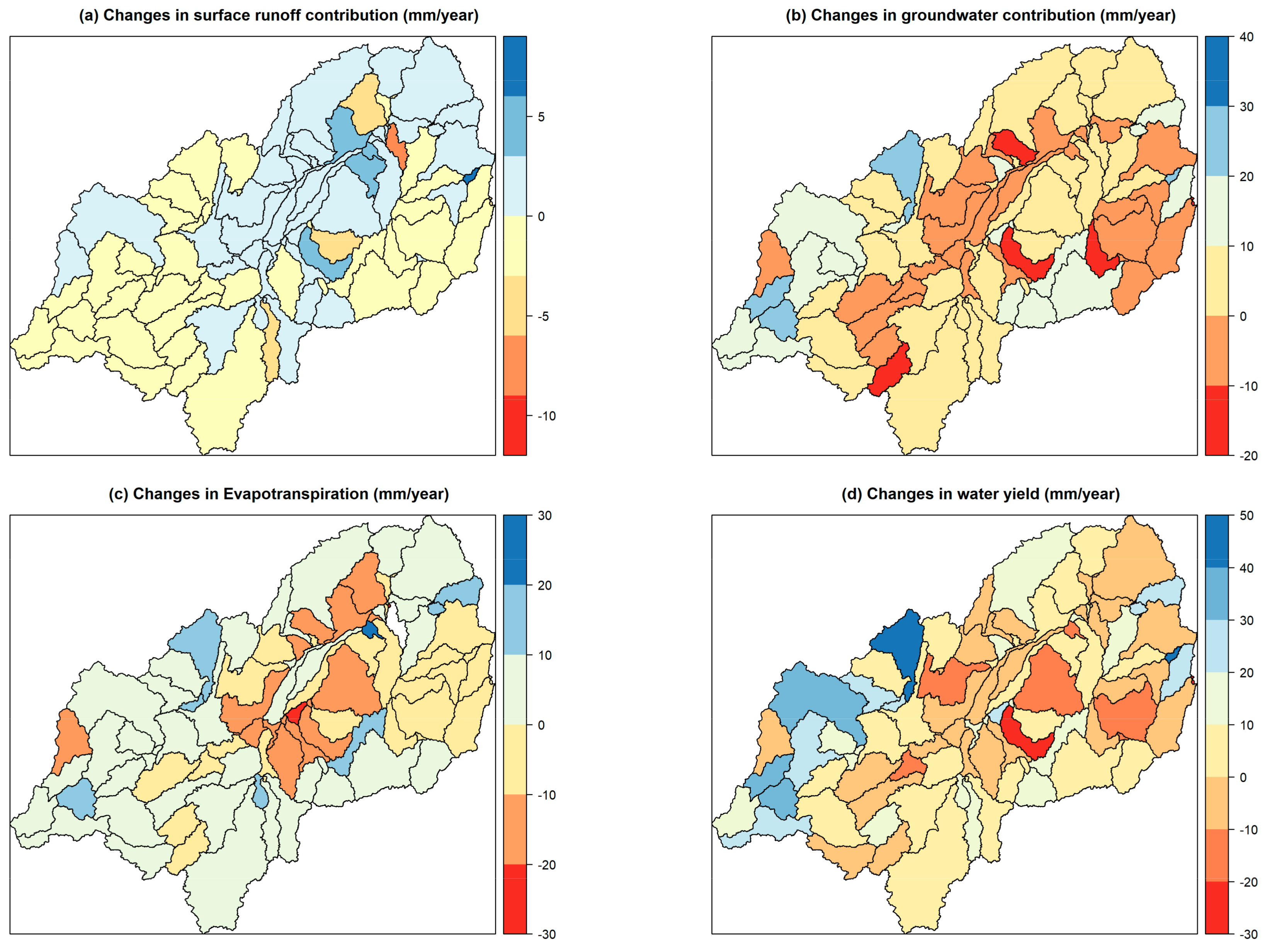
3.3. Land Use and Land Cover Changes and Their Impact on Water Resources
4. Discussion
4.1. Model Evaluation and Spatio-Temporal Analysis
4.2. Impact of Land Use and Land Cover Change
5. Conclusions
Author Contributions
Funding
Acknowledgments
Conflicts of Interest
References
- Leemhuis, C.; Amler, E.; Diekkrüger, B.; Gabiri, G.; Näschen, K. East African wetland-catchment data base for sustainable wetland management. Proc. Int. Assoc. Hydrol. Sci. 2016, 374, 123–128. [Google Scholar] [CrossRef]
- Sakané, N.; Alvarez, M.; Becker, M.; Böhme, B.; Handa, C.; Kamiri, H.W.; Langensiepen, M.; Menz, G.; Misana, S.; Mogha, N.G.; et al. Classification, characterisation, and use of small wetlands in East Africa. Wetlands 2011, 31, 1103–1116. [Google Scholar] [CrossRef]
- Ulrich, A. Export-oriented horticultural production in Laikipia, Kenya: Assessing the implications for rural livelihoods. Sustainability 2014, 6, 336–347. [Google Scholar] [CrossRef]
- Jew, E.; Bonnington, C. Socio-demographic factors influence the attitudes of local residents towards trophy hunting activities in the Kilombero Valley, Tanzania. Afr. J. Ecol. 2011, 49, 277–285. [Google Scholar] [CrossRef]
- Gabiri, G.; Diekkrüger, B.; Leemhuis, C.; Burghof, S.; Näschen, K.; Asiimwe, I.; Bamutaze, Y. Determining hydrological regimes in an agriculturally used tropical inland valley wetland in Central Uganda using soil moisture, groundwater, and digital elevation data. Hydrol. Process. 2017, 32, 349–362. [Google Scholar] [CrossRef]
- Munishi-Kongo, S. Ground and Satellite-Based Assessment of Hydrological Responses to Land Cover Change in the Kilombero River Basin, Tanzania. Ph.D. Thesis, University of KwaZulu-Natal, Pietermaritzburg, South Africa, November 2013. [Google Scholar]
- Beuel, S.; Alvarez, M.; Amler, E.; Behn, K.; Kotze, D.; Kreye, C.; Leemhuis, C.; Wagner, K.; Willy, D.K.; Ziegler, S.; et al. A rapid assessment of anthropogenic disturbances in East African wetlands. Ecol. Indic. 2016, 67, 684–692. [Google Scholar] [CrossRef]
- McCartney, M.; Rebelo, L.M.; Senaratna Sellamuttu, S.; de Silva, S. Wetlands, Agriculture and Poverty Reduction; IWMI Research Report 137; IWMI: Colombo, Sri Lanka, 2010. [Google Scholar] [CrossRef]
- Godfray, H.C.J.; Beddington, J.R.; Crute, I.R.; Haddad, L.; Lawrence, D.; Muir, J.F.; Pretty, J.; Robinson, S.; Thomas, S.M.; Toulmin, C. Food security: The challenge of feeding 9 billion people. Science 2010, 327, 812–818. [Google Scholar] [CrossRef] [PubMed]
- Schulla, J. Model Description WaSiM; Schulla, J., Ed.; Hydrology Software Consulting J. Schulla: Zürich, Switzerland, 2017. [Google Scholar]
- Arnold, J.G.; Srinivasan, R.; Muttiah, R.S.; Williams, J.R. Large area hydrologic modeling and assessment part I: Model Development. J. Am. Water Resour. Assoc. 1998, 34, 73–89. [Google Scholar] [CrossRef]
- Refsgaard, J.C.; Storm, B. MIKE SHE. In Computer Models of Watershed Hydrology; Singh, V.P., Ed.; Water Resources Publications: Highlands Ranch, CO, USA, 1995; pp. 809–846. ISBN 0918334918. [Google Scholar]
- Poméon, T.; Jackisch, D.; Diekkrüger, B. Evaluating the performance of remotely sensed and reanalysed precipitation data over West Africa using HBV light. J. Hydrol. 2017, 547, 222–235. [Google Scholar] [CrossRef]
- Montzka, C.; Canty, M.; Kunkel, R.; Menz, G.; Vereecken, H.; Wendland, F. Modelling the water balance of a mesoscale catchment basin using remotely sensed land cover data. J. Hydrol. 2008, 353, 322–334. [Google Scholar] [CrossRef]
- Mango, L.M.; Melesse, A.M.; McClain, M.E.; Gann, D.; Setegn, S.G. Land use and climate change impacts on the hydrology of the upper Mara River Basin, Kenya: Results of a modeling study to support better resource management. Hydrol. Earth Syst. Sci. 2011, 15, 2245–2258. [Google Scholar] [CrossRef]
- Bossa, A.Y.; Diekkrüger, B.; Agbossou, E.K. Scenario-based impacts of land use and climate change on land and water degradation from the meso to regional scale. Water 2014, 6, 3152–3181. [Google Scholar] [CrossRef]
- Wagner, P.D.; Kumar, S.; Schneider, K. An assessment of land use change impacts on the water resources of the Mula and Mutha Rivers catchment upstream of Pune, India. Hydrol. Earth Syst. Sci. 2013, 17, 2233–2246. [Google Scholar] [CrossRef]
- Baker, T.J.; Miller, S.N. Using the Soil and Water Assessment Tool (SWAT) to assess land use impact on water resources in an East African watershed. J. Hydrol. 2013, 486, 100–111. [Google Scholar] [CrossRef]
- Cornelissen, T.; Diekkrüger, B.; Giertz, S. A comparison of hydrological models for assessing the impact of land use and climate change on discharge in a tropical catchment. J. Hydrol. 2013, 498, 221–236. [Google Scholar] [CrossRef]
- Alemayehu, T.; van Griensven, A.; Bauwens, W. Improved SWAT vegetation growth module for tropical ecosystem. Hydrol. Earth Syst. Sci. 2017, 21, 4449–4467. [Google Scholar] [CrossRef]
- Mashingia, F.; Mtalo, F.; Bruen, M. Validation of remotely sensed rainfall over major climatic regions in Northeast Tanzania. Phys. Chem. Earth 2014, 67, 55–63. [Google Scholar] [CrossRef]
- Notter, B.; Hurni, H.; Wiesmann, U.; Ngana, J.O. Evaluating watershed service availability under future management and climate change scenarios in the Pangani Basin. Phys. Chem. Earth 2013, 61, 1–11. [Google Scholar] [CrossRef]
- Wambura, F.J.; Ndomba, P.M.; Kongo, V.; Tumbo, S.D. Uncertainty of runoff projections under changing climate in Wami River sub-basin. J. Hydrol. Reg. Stud. 2015, 4, 333–348. [Google Scholar] [CrossRef]
- Yawson, D.K.; Kongo, V.M.; Kachroo, R.K. Application of linear and nonlinear techniques in river flow forecasting in the Kilombero River basin, Tanzania. Hydrol. Sci. J. 2005, 50, 37–41. [Google Scholar] [CrossRef]
- Lyon, S.W.; Koutsouris, A.; Scheibler, F.; Jarsjö, J.; Mbanguka, R.; Tumbo, M.; Robert, K.K.; Sharma, A.N.; van der Velde, Y. Interpreting characteristic drainage timescale variability across Kilombero Valley, Tanzania. Hydrol. Process. 2015, 29, 1912–1924. [Google Scholar] [CrossRef]
- Burghof, S.; Gabiri, G.; Stumpp, C.; Chesnaux, R.; Reichert, B. Development of a hydrogeological conceptual wetland model in the data-scarce north-eastern region of Kilombero Valley, Tanzania. Hydrogeol. J. 2017, 26, 267–284. [Google Scholar] [CrossRef]
- Koutsouris, A. Building a Coherent Hydro-Climatic Modelling Framework for the Data Limited Kilombero Valley of Tanzania. Ph.D. Thesis, Stockholm University, Stockholm, Sweden, June 2017. [Google Scholar]
- Daniel, S.; Gabiri, G.; Kirimi, F.; Glasner, B.; Näschen, K.; Leemhuis, C.; Steinbach, S.; Mtei, K. Spatial Distribution of Soil Hydrological Properties in the Kilombero Floodplain, Tanzania. Hydrology 2017, 4, 57. [Google Scholar] [CrossRef]
- Seibert, J.; Vis, M.J.P. Teaching hydrological modeling with a user-friendly catchment-runoff-model software package. Hydrol. Earth Syst. Sci. 2012, 16, 3315–3325. [Google Scholar] [CrossRef] [Green Version]
- Leemhuis, C.; Thonfeld, F.; Näschen, K.; Steinbach, S.; Muro, J.; Strauch, A.; López, A.; Daconto, G.; Games, I.; Diekkrüger, B. Sustainability in the food-water-ecosystem nexus: The role of land use and land cover change for water resources and ecosystems in the Kilombero Wetland, Tanzania. Sustainability 2017, 9, 1513. [Google Scholar] [CrossRef]
- Muro, J.; Canty, M.; Conradsen, K.; Hüttich, C.; Nielsen, A.A.; Skriver, H.; Remy, F.; Strauch, A.; Thonfeld, F.; Menz, G. Short-term change detection in wetlands using Sentinel-1 time series. Remote Sens. 2016, 8, 795. [Google Scholar] [CrossRef]
- Wilson, E.; McInnes, R.; Mbaga, D.P.; Ouedaogo, P. Ramsar Advisory Mission Report; Ramsar Advisory Mission Report: Gland, Switzerland; Kilombero Valley, Tanzania, 2017. [Google Scholar]
- Mombo, F.; Speelman, S.; Van Huylenbroeck, G.; Hella, J.; Moe, S. Ratification of the Ramsar convention and sustainable wetlands management: Situation analysis of the Kilombero Valley wetlands in Tanzania. J. Agric. Ext. Rural Dev. 2011, 3, 153–164. [Google Scholar]
- Kangalawe, R.Y.M.; Liwenga, E.T. Livelihoods in the wetlands of Kilombero Valley in Tanzania: Opportunities and challenges to integrated water resource management. Phys. Chem. Earth Parts A/B/C 2005, 30, 968–975. [Google Scholar] [CrossRef]
- Ramsar Information Sheet. Information Sheet on Ramsar Wetlands (RIS). In Proceedings of the 8th Conference of the Contracting Parties to the Ramsar Convention (COP-8), Valencia, Spain, 18–26 November 2002. [Google Scholar]
- Gabiri, G.; Burghof, S.; Diekkrüger, B.; Steinbach, S.; Näschen, K. Modeling Spatial Soil Water Dynamics in a Tropical Floodplain, East Africa. Water 2018, 10, 191. [Google Scholar] [CrossRef]
- Government of Tanzania. Southern Agricultural Growth Corridor of Tanzania (SAGCOT): Environmental and Social Management Framework (ESMF); Government of Tanzania: Dodoma, Tanzania, 2013; p. 175.
- Koutsouris, A.J.; Chen, D.; Lyon, S.W. Comparing global precipitation data sets in eastern Africa: A case study of Kilombero Valley, Tanzania. Int. J. Climatol. 2016, 36, 2000–2014. [Google Scholar] [CrossRef]
- Camberlin, P.; Philippon, N. The East African March–May Rainy Season: Associated Atmospheric Dynamics and Predictability over the 1968–97 Period. J. Clim. 2002, 15, 1002–1019. [Google Scholar] [CrossRef]
- Nicholson, S.E. The nature of rainfall variability over Africa on time scales of decades to millenia. Glob. Planet. Chang. 2000, 26, 137–158. [Google Scholar] [CrossRef]
- Dewitte, O.; Jones, A.; Spaargaren, O.; Breuning-Madsen, H.; Brossard, M.; Dampha, A.; Deckers, J.; Gallali, T.; Hallett, S.; Jones, R.; et al. Harmonisation of the soil map of Africa at the continental scale. Geoderma 2013, 211, 138–153. [Google Scholar] [CrossRef] [Green Version]
- Zemandin, B.; Mtalo, F.; Mkhandi, S.; Kachroo, R.; McCartney, M. Evaporation Modelling in Data Scarce Tropical Region of the Eastern Arc Mountain Catchments of Tanzania. Nile Basin Water Sci. Eng. J. 2011, 4, 1–13. [Google Scholar]
- Kato, F. Development of a major rice cultivation area in the Kilombero Valley, Tanzania. Afr. Study Monogr. 2007, 36, 3–18. [Google Scholar] [CrossRef]
- Nindi, S.J.; Maliti, H.; Bakari, S.; Kija, H.; Machoke, M. Conflicts over Land and Water in the Kilombero Valley Floodplain, Tanzania. Afr. Study Monogr. 2014, 50, 173–190. [Google Scholar] [CrossRef]
- Gutowski, J.W.; Giorgi, F.; Timbal, B.; Frigon, A.; Jacob, D.; Kang, H.S.; Raghavan, K.; Lee, B.; Lennard, C.; Nikulin, G.; et al. WCRP COordinated Regional Downscaling EXperiment (CORDEX): A diagnostic MIP for CMIP6. Geosci. Model Dev. 2016, 9, 4087–4095. [Google Scholar] [CrossRef]
- Dee, D.P.; Uppala, S.M.; Simmons, A.J.; Berrisford, P.; Poli, P.; Kobayashi, S.; Andrae, U.; Balmaseda, M.A.; Balsamo, G.; Bauer, P.; et al. The ERA-Interim reanalysis: Configuration and performance of the data assimilation system. Q. J. R. Meteorol. Soc. 2011, 137, 553–597. [Google Scholar] [CrossRef]
- United States Geological Survey (USGS). Available online: https://earthexplorer.usgs.gov/ (accessed on 8 December 2016).
- Breiman, L. Random forests. Mach. Learn. 2001, 45, 5–32. [Google Scholar] [CrossRef]
- USGS Department of the Interior Product Guide—Landsat 4–7 Surface Reflectance (LEDAPS) Product Version 8.3. Available online: https://landsat.usgs.gov/sites/default/files/documents/ledaps_product_guide.pdf (accessed on 18 April 2018).
- USGS Department of the Interior Product Guide Landsat 8 Surface Reflectance Code (LASRC) Product Version 4.3. Available online: https://landsat.usgs.gov/sites/default/files/documents/lasrc_product_guide.pdf (accessed on 18 April 2018).
- Crist, E.P. A TM Tasseled Cap equivalent transformation for reflectance factor data. Remote Sens. Environ. 1985, 17, 301–306. [Google Scholar] [CrossRef]
- Crist, E.P.; Cicone, R.C. A Physically-Based Transformation of Thematic Mapper Data—The TM Tasseled Cap. IEEE Trans. Geosci. Remote Sens. 1984, 22, 256–263. [Google Scholar] [CrossRef]
- Yamamoto, K.H.; Finn, M.P. Approximating Tasseled Cap Values to Evaluate Brightness, Greenness, and Wetness for the Advanced Land Imager (ALI); Scientific Investigations Report; USGS: Reston, VA, USA, 2012. [Google Scholar]
- McFeeters, S.K. The use of the Normalized Difference Water Index (NDWI) in the delineation of open water features. Int. J. Remote Sens. 1996, 17, 1425–1432. [Google Scholar] [CrossRef]
- Tucker, C.J. Red and photographic infrared linear combinations for monitoring vegetation. Remote Sens. Environ. 1979, 8, 127–150. [Google Scholar] [CrossRef]
- Lehner, B.; Verdin, K.; Jarvis, A. New Global Hydrography Derived From Spaceborne Elevation Data. Eos Trans. Am. Geophys. Union 2008, 89, 93. [Google Scholar] [CrossRef]
- Riley, S.J.; DeGloria, S.D.; Elliot, R. A terrain ruggedness index that quantifies topographic heterogeneity. Int. J. Sci. 1999, 5, 23–27. [Google Scholar]
- Ruszkiczay-Rüdiger, Z.; Fodor, L.; Horváth, E.; Telbisz, T. Discrimination of fluvial, eolian and neotectonic features in a low hilly landscape: A DEM-based morphotectonic analysis in the Central Pannonian Basin, Hungary. Geomorphology 2009, 104, 203–217. [Google Scholar] [CrossRef]
- Gallant, J.C.; Wilson, J.P. Primary topographic attributes. In Terrain Analysis: Principles and Applications; Wilson, J.P., Gallant, J.C., Eds.; John Wiley & Sons: New York, NY, USA, 2000; pp. 51–85. [Google Scholar]
- Jenness, J. Topographic Position Index (tpi_jen.avx) Extension for ArcView 3.x, Version 1.2; Jenness Enterprises: Flagstaff, AZ, USA, 2006. [Google Scholar]
- Beven, K.J.; Kirkby, M.J. A physically based, variable contributing area model of basin hydrology/Un modèle à base physique de zone d’appel variable de l’hydrologie du bassin versant. Hydrol. Sci. J. 1979, 24, 43–69. [Google Scholar] [CrossRef]
- RBWO; The Rufiji Basin Water Office (RBWO) Discharge Database; Rufiji Basin Water Office (RBWO): Iringa, Tanzania. Personal Communication, 2014.
- Neitsch, S.L.; Arnold, J.G.; Kiniry, J.R.; Williams, J.R. Soil & Water Assessment Tool Theoretical Documentation Version 2009; Neitsch, S.L., Arnold, J.G., Kiniry, J.R., Williams, J.R., Eds.; Grassland, Soil and Water Research Laboratory: Temple, TX, USA, 2011. [Google Scholar]
- Soil Conservation Service (Ed.) Hydrology. In National Engineering Handbook; Soil Conservation Service: Washington, DC, USA, 1972. [Google Scholar]
- Monteith, J.L.; Moss, C.J. Climate and the Efficiency of Crop Production in Britain. Philos. Trans. R. Soc. B Biol. Sci. 1977, 281, 277–294. [Google Scholar] [CrossRef]
- Sloan, P.G.; Moore, I.D. Modeling subsurface stormflow on steeply sloping forested watersheds. Water Resour. Res. 1984, 20, 1815–1822. [Google Scholar] [CrossRef]
- Arnold, J.G.; Kiniry, J.; Srinivasan, R.; Williams, J.R.; Haney, E.B.; Neitsch, S.L. Soil and Water Assessment Tool Input/Output File Documentation Version 2009; No. 365; Texas Water Resources Institute: College Station, TX, USA, 2011; pp. 1–662. [Google Scholar]
- Arnold, J.G.; Kiniry, J.R.; Srinivasan, R.; Williams, J.R.; Haney, E.B.; Neitsch, S.L. Soil & Water Assessment Tool: Input/Output Documentation Version 2012; No. 439; Texas Water Resources Institute: College Station, TX, USA, 2012; pp. 1–650. [Google Scholar]
- Abbaspour, K.C. SWAT-CUP 2012. SWAT Calibration and Uncertainty Programs; Abbaspour, K.C., Ed.; Eawag: Dübendorf, Switzerland, 2013. [Google Scholar]
- Arnold, J.G.; Moriasi, D.N.; Gassman, P.W.; Abbaspour, K.C.; White, M.; Srinivasan, R.; Santhi, C.; Harmel, R.D.; van Griensven, A.; Van Liew, M.W.; et al. SWAT: Model use, calibration, and validation. Trans. ASABE 2012, 55, 1491–1508. [Google Scholar] [CrossRef]
- Abbaspour, K.C.; Rouholahnejad, E.; Vaghefi, S.; Srinivasan, R.; Yang, H.; Kløve, B. A Continental-Scale Hydrology and Water Quality Model for Europe: Calibration and uncertainty of a high-resolution large-scale SWAT model. J. Hydrol. 2015, 524, 733–752. [Google Scholar] [CrossRef]
- Gupta, H.V.; Kling, H.; Yilmaz, K.K.; Martinez, G.F. Decomposition of the mean squared error and NSE performance criteria: Implications for improving hydrological modelling. J. Hydrol. 2009, 377, 80–91. [Google Scholar] [CrossRef]
- Nash, J.E.; Sutcliffe, J.V. River flow forecasting through conceptual models part I—A discussion of principles. J. Hydrol. 1970, 10, 282–290. [Google Scholar] [CrossRef]
- Gupta, H.V.; Sorooshian, S.; Yapo, P.O. Status of Automatic Calibration for Hydrologic Models: Comparison With Multilevel Expert Calibration. J. Hydrol. Eng. 1999, 4, 135–143. [Google Scholar] [CrossRef]
- Huffman, G.J.; Bolvin, D.T.; Nelkin, E.J.; Wolff, D.B.; Adler, R.F.; Gu, G.; Hong, Y.; Bowman, K.P.; Stocker, E.F.; Huffman, G.J.; et al. The TRMM Multisatellite Precipitation Analysis (TMPA): Quasi-Global, Multiyear, Combined-Sensor Precipitation Estimates at Fine Scales. J. Hydrometeorol. 2007, 8, 38–55. [Google Scholar] [CrossRef]
- Arnold, J.G.; Allen, P.M.; Muttiah, R.; Bernhardt, G. Automated Base Flow Separation and Recession Analysis Techniques. Groundwater 1995, 33, 1010–1018. [Google Scholar] [CrossRef]
- Nicholson, S.E. A review of climate dynamics and climate variability in Eastern Africa. In Limnology, Climatology and Paleoclimatology of the East African Lakes; Gordon and Breach Publishers, Inc.: Philadelphia, PA, USA, 1996; pp. 25–26. [Google Scholar]
- Nyenzi, B.S.; Kiangi, P.M.R.; Rao, N.N.P. Evaporation values in East Africa. Arch. Meteorol. Geophys. Bioclimatol. Ser. B 1981, 29, 37–55. [Google Scholar] [CrossRef]
- Moriasi, D.N.; Gitau, M.W.; Pai, N.; Daggupati, P. Hydrologic and Water Quality Models: Performance Measures and Evaluation Criteria. Trans. ASABE 2015, 58, 1763–1785. [Google Scholar] [CrossRef]
- MacDonald, A.M.; Bonsor, H.C. Groundwater and Climate Change in Africa: Review of Recharge Studies; British Geological Survey: Nottingham, UK, 2010. [Google Scholar]
- Dagg, M.; Woodhead, T.; Rijks, D.A. Evaporation in East Africa. Hydrol. Sci. J. 1970, 15, 61–67. [Google Scholar] [CrossRef]
- Beven, K.J. Rainfall-Runoff Modelling: The Primer, 2nd ed.; Wiley-Blackwell: Hoboken, NJ, USA, 2012. [Google Scholar]
- Tang, Q.; Gao, H.; Lu, H.; Lettenmaier, D.P. Remote sensing: hydrology. Prog. Phys. Geogr. 2009, 33, 490–509. [Google Scholar] [CrossRef]
- Becker, A.; Finger, P.; Meyer-Christoffer, A.; Rudolf, B.; Schamm, K.; Schneider, U.; Ziese, M. A description of the global land-surface precipitation data products of the Global Precipitation Climatology Centre with sample applications including centennial (trend) analysis from 1901-present. Earth Syst. Sci. Data 2013, 5, 71–99. [Google Scholar] [CrossRef]
- Rienecker, M.M.; Suarez, M.J.; Gelaro, R.; Todling, R.; Bacmeister, J.; Liu, E.; Bosilovich, M.G.; Schubert, S.D.; Takacs, L.; Kim, G.-K.; et al. MERRA: NASA’s Modern-Era Retrospective Analysis for Research and Applications. J. Clim. 2011, 24, 3624–3648. [Google Scholar] [CrossRef]
- Adjei, K.A.; Ren, L.; Appiah-Adjei, E.K.; Odai, S.N. Application of satellite-derived rainfall for hydrological modelling in the data-scarce Black Volta trans-boundary basin. Hydrol. Res. 2015, 46, 777–791. [Google Scholar] [CrossRef]
- Legates, D.R.; McCabe, G.J., Jr. Evaluating the Use of “Goodness of Fit” Measures in Hydrologic and Hydroclimatic Model Validation. Water Resour. Res. 1999, 35, 233–241. [Google Scholar] [CrossRef]
- Troch, P.A.; Berne, A.; Bogaart, P.; Harman, C.; Hilberts, A.G.J.; Lyon, S.W.; Paniconi, C.; Pauwels, V.R.N.; Rupp, D.E.; Selker, J.S.; et al. The importance of hydraulic groundwater theory in catchment hydrology: The legacy of Wilfried Brutsaert and Jean-Yves Parlange. Water Resour. Res. 2013, 49, 5099–5116. [Google Scholar] [CrossRef] [Green Version]
- Yira, Y.; Diekkrüger, B.; Steup, G.; Bossa, A.Y. Modeling land use change impacts on water resources in a tropical West African catchment (Dano, Burkina Faso). J. Hydrol. 2016, 537, 187–199. [Google Scholar] [CrossRef]
- Bossa, A.Y.; Diekkrüger, B.; Igué, A.M.; Gaiser, T. Analyzing the effects of different soil databases on modeling of hydrological processes and sediment yield in Benin (West Africa). Geoderma 2012, 173, 61–74. [Google Scholar] [CrossRef]
- Ndomba, P.; Mtalo, F.; Killingtveit, A. SWAT model application in a data scarce tropical complex catchment in Tanzania. Phys. Chem. Earth Parts A/B/C 2008, 33, 626–632. [Google Scholar] [CrossRef]
- Strauch, M.; Volk, M. SWAT plant growth modification for improved modeling of perennial vegetation in the tropics. Ecol. Model. 2013, 269, 98–112. [Google Scholar] [CrossRef]
- Burghof, S. Hydrogeology and Water Quality of Wetlands in East Africa. Ph.D. Thesis, University of Bonn, Bonn, Germany, May 2017. [Google Scholar]
- Vogelmann, J.E.; Gallant, A.L.; Shi, H.; Zhu, Z. Perspectives on monitoring gradual change across the continuity of Landsat sensors using time-series data. Remote Sens. Environ. 2016, 185, 258–270. [Google Scholar] [CrossRef]
- Hecheltjen, A.; Thonfeld, F.; Menz, G. Recent advances in remote sensing change detection—A review. In Land Use and Land Cover Mapping in Europe. Practices & Trends; Manakos, I., Braun, M., Eds.; Springer: Berlin, Germany, 2014; pp. 145–178. [Google Scholar]
- Lal, R. Deforestation effects on soil degradation and rehabilitation in western Nigeria. IV. Hydrology and water quality. Land Degrad. Dev. 1997, 8, 95–126. [Google Scholar] [CrossRef]
- WREM International Inc. Rufiji Basin IWRMD Plan: Draft Interim Report II. Executive Summary: Preliminary Assessment Findings and Planning Recommendations; WREM International Inc.: Atlanta, GA, USA, 2013. [Google Scholar]
- Wilk, J.; Hughes, D.A. Simulating the impacts of land-use and climate change on water resource availability for a large south Indian catchment. Hydrol. Sci. J. 2002, 47, 19–30. [Google Scholar] [CrossRef]
- Wagner, P.D. Impacts of Climate Change and Land Use Change on the Water Resources of the Mula and Mutha Rivers Catchment upstream of Pune, India. Ph.D. Thesis, University of Cologne, Cologne, Germany, January 2013. [Google Scholar]
- Benjaminsen, T.A.; Maganga, F.P.; Abdallah, J.M. The Kilosa Killings: Political Ecology of a Farmer-Herder Conflict in Tanzania. Dev. Chang. 2009, 40, 423–445. [Google Scholar] [CrossRef]
- Bonarius, H. Physical properties of soils in the Kilombero Valley (Tanzania), In Schriftenreihe der GTZ 26; German Agency for Technical Cooperation: Eschborn, Germany, 1975; Volume 26, pp. 1–36. [Google Scholar]
- Funk, C.; Nicholson, S.E.; Landsfeld, M.; Klotter, D.; Peterson, P.; Harrison, L. The Centennial Trends Greater Horn of Africa precipitation dataset. Sci. Data 2015, 2, 150050. [Google Scholar] [CrossRef] [PubMed]
- Tang, Q.; Oki, T. Terrestrial Water Cycle and Climate Change: Natural and Human-Induced Impacts; Tang, Q., Oki, T., Eds.; Wiley: Hoboken, NJ, USA, 2016. [Google Scholar]


| Data Set | Resolution/Scale | Source | Required Parameters |
|---|---|---|---|
| DEM | 90 m | SRTM [56] | Topographical data |
| Soil map | 1 km | FAO [41] | Soil classes and physical properties |
| Land use maps | 60 m (1970s) 30 m (1994, 2004, 2014) | Landsat pre-Collection Level-1 [47], Landsat TM, ETM+, OLI Surface Reflectance Level-2 Science Products [49,50], SRTM [56] | Land cover and use classes |
| Precipitation | Daily | Personal communication: RBWB, University of Dar es Salaam (UDSM), Tanzania Meteorological Agency (TMA) | Rainfall |
| Climate | Daily/0.44° | CORDEX Africa [45] | Temperature, humidity, solar radiation, wind speed |
| Discharge | Daily (1958–1970) | RBWB [62] | Discharge |
| GCM | RCM | Institution | URL |
|---|---|---|---|
| CanESM2 | CanRCM4_r2 | Canadian Centre for Climate Modelling and Analysis (CCCma) | http://climate-modelling.canada.ca/ |
| CanESM2 | RCA4_v1 | Rossby Centre, Swedish Meteorological and Hydrological Institute (SMHI) | https://esg-dn1.nsc.liu.se/ |
| CNRM-CM5 | CCLM4-8-17_v1 | Climate Limited-area Modelling Community (CLMcom) | https://esg-dn1.nsc.liu.se/ |
| EC-EARTH | CCLM4-8-17_v1 | Climate Limited-area Modelling Community (CLMcom) | https://esg-dn1.nsc.liu.se/ |
| EC-EARTH | RCA4_v1 | Rossby Centre, Swedish Meteorological and Hydrological Institute (SMHI) | https://esg-dn1.nsc.liu.se/ |
| MIROC5 | RCA4_v1 | Rossby Centre, Swedish Meteorological and Hydrological Institute (SMHI) | https://esg-dn1.nsc.liu.se/ |
| Soil Type | Proportional Area (%) | LULC Class (1970s Land Use) | Proportional Area (%) | Slope Classes | Proportional Area (%) |
|---|---|---|---|---|---|
| Haplic Acrisol | 30.82% | Savanna | 45.30% | 0–2% | 22.45% |
| Eutric Fluvisol | 14.77% | Range-Grasses | 23.49% | 2%–5% | 12.09% |
| Humic Nitisol | 13.14% | Forest-Mixed | 22.05% | 5%–8% | 11.66% |
| Ferric Lixisol | 13.05% | Forest-Evergreen | 6.81% | 8%–12% | 13.96% |
| Ferric Acrisol | 9.08% | Agricultural Land | 1.20% | >12% | 39.85% |
| Humic Acrisol | 5.73% | Water | 0.95% | ||
| Albic Arenosol | 2.75% | Barren | 0.20% | ||
| Eutric Leptosol | 0.59% |
| Rank | Parameter | Description | Final Range | Method |
|---|---|---|---|---|
| 1 | GWQMN.gw | Threshold depth of water in the shallow aquifer for return flow to occur (mm). | 1400–2200 | v |
| 2 | ALPHA_BF.gw | Base flow alpha factor (days). | 0.15–0.26 | v |
| 3 | GW_REVAP.gw | Groundwater “revap” coefficient. | 0.15–0.2 | v |
| 4 | SURLAG.bsn | Surface runoff lag coefficient. | 2.8–5.3 | v |
| 5 | GW_DELAY.gw | Groundwater delay time (days). | 4–30 | v |
| 6 | SOL_K().sol | Saturated hydraulic conductivity (mm/h). | 0.4–0.7 | r |
| 7 | RCHRG_DP.gw | Deep aquifer percolation fraction. | 0.31–0.37 | v |
| 8 | SOL_Z().sol | Depth from soil surface to bottom of layer (mm). | 0.35–0.5 | r |
| 9 | SOL_AWC().sol | Available water capacity of the soil layer (mm H2O/mm soil). | −0.1–0.13 | r |
| 10 | R__OV_N.hru | Manning’s “n” value for overland flow. | 0.1–0.2 | r |
| 11 | R__CN2.mgt | SCS runoff curve number for moisture condition II. | −0.5–(−0.35) | r |
| 12 | CH_K1.sub | Effective hydraulic conductivity in the tributary channel (mm/h). | 65–80 | v |
| 13 | ESCO.hru | Soil evaporation compensation factor. | 0–0.1 | v |
| 14 | CH_K2.rte | Effective hydraulic conductivity in the main channel (mm/h) | 100–130 | v |
| 15 | REVAPMN.gw | Threshold depth of water in the shallow aquifer for “revap” to occur (mm). | 13–30 | v |
| 16 | EPCO.hru | Plant uptake compensation factor. | 0.9–1 | v |
| 17 | PLAPS | Precipitation lapse rate (mm H2O/km). | 130 | v |
| 18 | TLAPS | Temperature lapse rate (°C/km). | −6 | v |
| Simulation Period(Daily) | P-Factor | R-Factor | R2 | NSE | PBIAS | KGE | RSR |
|---|---|---|---|---|---|---|---|
| Calibration (1958–1965) | 0.62 | 0.45 | 0.86 | 0.85 | 0.3 | 0.93 | 0.38 |
| Validation (1966–1970) | 0.67 | 0.56 | 0.80 | 0.80 | 2.5 | 0.89 | 0.45 |
| Water Balance Components | in (mm) |
|---|---|
| Precipitation | 1344 |
| Actual evapotranspiration | 788 |
| Potential evapotranspiration | 1380 |
| Surface runoff | 43 |
| Lateral flow | 58 |
| Base flow | 209 |
| Recharge to the deep aquifer | 242 |
© 2018 by the authors. Licensee MDPI, Basel, Switzerland. This article is an open access article distributed under the terms and conditions of the Creative Commons Attribution (CC BY) license (http://creativecommons.org/licenses/by/4.0/).
Share and Cite
Näschen, K.; Diekkrüger, B.; Leemhuis, C.; Steinbach, S.; Seregina, L.S.; Thonfeld, F.; Van der Linden, R. Hydrological Modeling in Data-Scarce Catchments: The Kilombero Floodplain in Tanzania. Water 2018, 10, 599. https://doi.org/10.3390/w10050599
Näschen K, Diekkrüger B, Leemhuis C, Steinbach S, Seregina LS, Thonfeld F, Van der Linden R. Hydrological Modeling in Data-Scarce Catchments: The Kilombero Floodplain in Tanzania. Water. 2018; 10(5):599. https://doi.org/10.3390/w10050599
Chicago/Turabian StyleNäschen, Kristian, Bernd Diekkrüger, Constanze Leemhuis, Stefanie Steinbach, Larisa S. Seregina, Frank Thonfeld, and Roderick Van der Linden. 2018. "Hydrological Modeling in Data-Scarce Catchments: The Kilombero Floodplain in Tanzania" Water 10, no. 5: 599. https://doi.org/10.3390/w10050599