Article

Assessing Long-Term Hydrological Impact of Climate Change Using an Ensemble Approach and Comparison with Global Gridded Model-A Case Study on Goodwater Creek Experimental Watershed

1
Department of Bioengineering, University of Missouri, Columbia, MO 65201, USA
2
Industrial & Manufacturing Systems Engineering, University of Missouri, Columbia, MO 65201, USA
3
USDA–ARS, Cropping Systems and Water Quality Research Unit, Columbia, MO 65211, USA
4
Salt River Project, Surface Water Resources, Tempe, AZ 85072, USA
*
Author to whom correspondence should be addressed.
Water 2018, 10(5), 564; https://doi.org/10.3390/w10050564
Submission received: 19 March 2018 / Revised: 19 April 2018 / Accepted: 24 April 2018 / Published: 26 April 2018

Abstract

:
Potential impacts of climate change on the hydrological components of the Goodwater Creek Experimental Watershed were assessed using climate datasets from the Coupled Model Intercomparison Project Phase 5 and Soil and Water Assessment Tool (SWAT). Historical and future ensembles of downscaled precipitation and temperature, and modeled water yield, surface runoff, and evapotranspiration, were compared. Ensemble SWAT results indicate increased springtime precipitation, water yield, surface runoff and a shift in evapotranspiration peak one month earlier in the future. To evaluate the performance of model spatial resolution, gridded surface runoff estimated by Lund–Potsdam–Jena managed Land (LPJmL) and Jena Diversity-Dynamic Global Vegetation model (JeDi-DGVM) were compared to SWAT. Long-term comparison shows a 6–8% higher average annual runoff prediction for LPJmL, and a 5–30% lower prediction for JeDi-DGVM, compared to SWAT. Although annual runoff showed little change for LPJmL, monthly runoff projection under-predicted peak runoff and over-predicted low runoff for LPJmL compared to SWAT. The reasons for these differences include differences in spatial resolution of model inputs and mathematical representation of the physical processes. Results indicate benefits of impact assessments at local scales with heterogeneous sets of parameters to adequately represent extreme conditions that are muted in global gridded model studies by spatial averaging over large study domains.

1. Introduction

Climatic shift due to anthropogenic activities has been linked to water supply shortages [1,2], declining biodiversity [3,4,5], ecosystem damage [6], and economic impact [7]. Increased greenhouse gas (GHG) concentrations alter the radiative balance of the Earth’s atmosphere, causing an increase in average temperature (T) and changes in precipitation (P) patterns [8,9]. The Intergovernmental Panel on Climate Change (IPCC) reports increases in mean surface temperature of between 0.3 and 4.8 °C by 2081–2100 relative to 1986–2005, and variable changes in precipitation across the globe for the same period of comparison [10], dependent upon GHG concentrations in the atmosphere. The atmospheric carbon dioxide (CO2) concentration is estimated to increase from the present day concentration of approximately 400 ppm to approximately 850 ppm by year 2075 in the highest emission scenario (RCP 8.5) [10]. The projected changes in meteorological variables have been reported to impact hydrological components, and ultimately agroecosystem functioning [11,12,13]. The majority of modeling exercises have been conducted at larger scales than this study, despite the fact that in reality, management decisions are taken at a local scale by individual farmers. Therefore, it is important to develop approaches to increase the ability to predict how future climate changes could impact hydrological components, and correspondingly, agricultural productivity, through the representation of localized systems.
Multiple Global Circulation Models (GCMs) have been developed to project future Earth climate given multiple plausible futures [10]. GCMs are three-dimensional numerical models that represent the physical dynamics of the atmosphere, ocean, cryosphere, and land surface, and are the best available methods for predicting how these systems behave given increasing GHG concentrations in the atmosphere [14]. In the Fifth Assessment Report, the climate projections are organized into four Representative Concentration Pathways (RCPs) (RCP 2.6, RCP 4.5, RCP 6.0, and RCP 8.5) based on radiative forcing levels associated with socioeconomic and technical assumptions by the end of the century [15]. Radiative forcing is defined as the difference between incoming solar radiation and outgoing infrared radiation caused by increased concentration of GHGs expressed in Watts per square meter (W/m2) [16]. Note that climate change impact assessment studies using hydrological models include different sources of uncertainty: uncertainty in future climate projections (GCM), downscaling techniques, and hydrological modeling [17,18].
Hydrological models have been used to simulate the long-term impact of projected changes in climate to assist with the quantification of future risk and, if necessary, to assist with developing adaptive management strategies [19,20]. Hydrological simulation models have been applied to assess the impacts of climate change on nutrient loading [21], crop productivity [22], and streamflow [23,24]. The majority of climate impact assessment studies have been conducted at larger scales using gridded model structures matching with the resolution of Coupled Model Intercomparison Project (CMIP3 and CMIP5) [22,24,25,26]. Studies in the Midwestern United States have focused on quantifying the impact of future climate on hydrological processes at a regional scale using gridded climate data (50 × 50 km) [18,27,28] and with some studies conducted in mid-sized watersheds [29,30,31]. There have been relatively few studies at smaller scales [32,33,34], in part due to lack of fine resolution climate model output and corresponding, data-intensive requirements to further downscale these data to a specific location to use in hydrological models for local scale applications [19]. Watershed sizes were defined using United States Geological Survey (USGS) classification scheme based on hydrological unit code (HUC) which consists of six levels of classification [35]. Specifically, subwatershed to watershed (~100 km2 to 585), subbasin to basin (>585 to 27,445 km2), and sub region to region (>27,445 km2 and above) were considered as local scale, mid-size and regional scale, respectively.
Hydrological components can be simulated at various scales. The spatial and temporal scale of a hydrological model also defines the resolution of key output variables. For regional reservoir managers, a coarser resolution of both space and time may be sufficient for anticipating and planning for predicting water levels. For example, the Variable Infiltration Capacity (VIC) model [36] operates at a 10-kmgrid cell size and a daily time-step, and is useful for regional-scale water management planning and identification of general trends. In contrast, the Agricultural Policy Environmental eXtender (APEX) model [37] operates at field scale (a few to few hundreds of hectares), and is useful for field-scale management planning. Thus, hydrological models can produce distinct results, because of the model structure, parametrization and resolution of inputs [38,39]. Comparison of model results at multiple scales can help to evaluate which resolution is necessary and appropriate for particular risk and adaptation questions. For example, early work on hydrological impacts associated with future climate change have focused on determining which regions of countries and even the globe may be at risk of changes in water availability, a question for which a coarse resolution may be adequate. However, in order to develop strategic responses in a specific location, and particularly the need to link hydrology to agricultural productivity, a finer resolution may be required in order to evaluate low probability, high risk events (e.g., flooding, drought, etc.). Similarly, a finer resolution for key parameters representing physical processes is likely to result in an increased ability to predict responses to future climate conditions.
The geographic focus of this study is the Goodwater Creek Experimental Watershed (GCEW), which is part of a Long Term Agroecosystem Research (LTAR) site, and has been a part of a broader USDA-ARS watershed network since 1971; thus, it has ample, high quality data [40]. The Soil Water Assessment Tool (SWAT) [41] has been used to model this watershed for many years in conjunction with this LTAR research program. The SWAT model [41] is a widely used watershed-scale process-based distributed parameter hydrological simulation model designed to simulate hydrological components, and enables detailed representation of agricultural land cover and management practices [42,43]. SWAT includes algorithms for predicting how P, T, and CO2 concentration affect plant growth and hydrological components.
The GCEW is a headwater watershed in the Salt River Basin, and the geophysical context of the study area represents the Central Claypan region, which includes Northeast Missouri, Southeast Iowa and Southern Illinois [40,44]. GCEW includes a restrictive clay layer in the subsurface soil (B-Horizon), which results in lower hydraulic conductivity, and ultimately, in considerable surface water runoff despite shallow slopes [45,46]. The presence of this restrictive clay layer may result in more significant responses in hydrological components as a result of future changes in T and P. For example, intense precipitation events could result in higher runoff, whereas short-term dry periods may result in short-term drought, both of which can impact agricultural productivity. Hydrological models with a coarse spatial resolution may not be able to adequately capture hydrological responses to climate in areas with unique physical features, such as the claypan in the GCEW.
The objectives of this study are to contribute to the body of knowledge developed in conjunction with the LTAR project in the GCEW, to characterize the potential hydrological impacts in relation to climate change in the GCEW, and to compare hydrological output from models of different spatial resolution, as well as with and without localized downscaling of weather data. This is an important inquiry for developing modeling techniques to assess risks to hydrological components and agricultural activity. To support these objectives, 12 climate model datasets obtained from CMIP5 were statistically downscaled using historic T and P data from GCEW [47] and modeled hydrological responses were analyzed using an ensemble approach. To support the last objective, SWAT simulated runoff was compared with simulated runoff from the Lund–Potsdam–Jena managed Land (LPJmL) and Jena Diversity-Dynamic Global Vegetation (JeDi-DGVM) models forced with precipitation data bias corrected using a nonlinear regression with a spatial resolution of 0.5 degree [48]. These data were made available via the Inter-Sectoral Impact Model Intercomparison Project (ISI-MIP) [49]. Runoff results were compared to evaluate the performance of these varying spatial resolutions, to generate more insight on why there is a need for detailed simulation with higher spatial resolution in an agricultural setup.

2. Materials and Methods

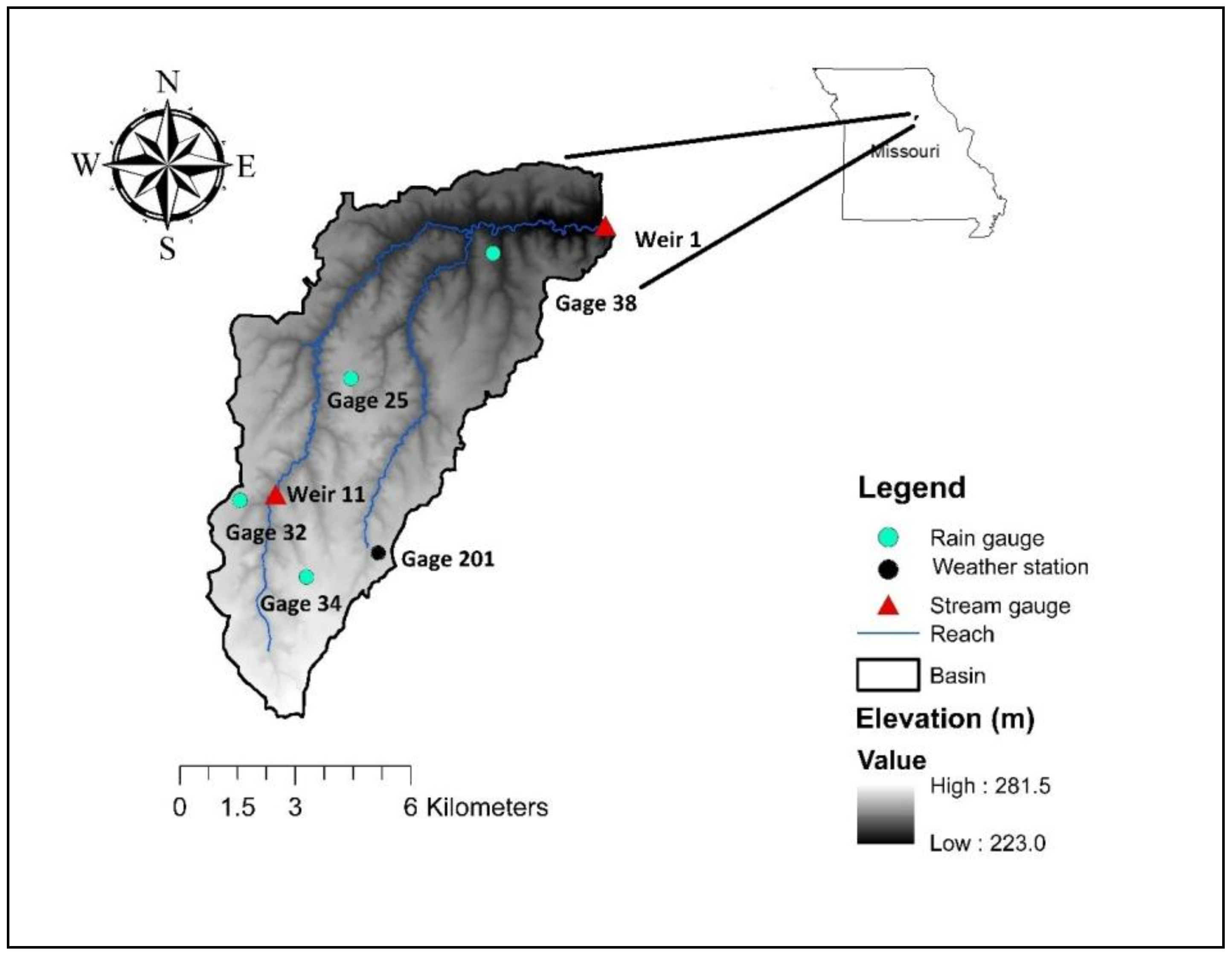
2.1. Watershed Description and Data Sources

The study was conducted in the GCEW, located in Boone and Audrain counties, Missouri (Figure 1), with a drainage area of approximately 73 km2 [40]. The land uses in the watershed include row crops (72.8% of total land area), pasture (14.3%), forest (6.0%), and urban land (6.9%) (Table 1). The study area received an average annual precipitation of 1027 mm between 1993 and 2010, with maximum and minimum annual precipitation of 1614 and 776 mm for 2008 and 2007 respectively [47]. The historical average annual estimated snowfall depth for the study watershed is around 380 mm; given the difficulty in obtaining snow measurements, snow water equivalent is measured in the study area [47]. The daily average maximum and minimum temperatures during this same period were 17.5 °C and 6.5 °C respectively. The average annual discharge of the watershed (expressed as a depth over the drainage area) is 310 mm, proportioned of surface (80%) and base flow (20%) [50].The watershed has flat topography, with 69% of the area having a slope of 0–2%, 15.2% having a slope of 2–3%, and the remaining 15.8% having a slope greater than 3%. The average elevation of the watershed is 256 m above sea level, ranging from 223 to 281 m.
Data required for the SWAT model included a Digital Elevation Model (DEM), soil database, Land Use/Land Cover (LULC), and weather datasets. The DEM (10-m resolution), soil (30-m resolution), and land use/land cover (30-m resolution) datasets were downloaded from Missouri Spatial Data Information Service (MSDIS) (http://msdis.missouri.edu/data/dem/) [51], Soil Survey Geographic Data (SSURGO) (http://websoilsurvey.sc.egov.usda.gov/App/WebSoilSurvey.aspx) data set [52], and National Agricultural Statistics Service (NASS) Cropland Data Layer (CDL) (http://nassgeodata.gmu.edu/CropScape/) of the United States Department of Agriculture (USDA) [53], respectively. The historical weather datasets required for the model, including daily P, daily maximum and minimum air T, wind speed, and solar radiation, were obtained from the weather station and rain gauge located in the watershed (Figure 1). The precipitation datasets from 5 different rain gauges (Figure 1) were used to better represent the spatial variability of precipitation across the watershed.

2.2. Description of SWAT Model and Model Setup for GCEW

The SWAT 2012 version 635 was used by incorporating the changes included in an earlier modeling effort to simulate the percolation through and saturation above the claypan [44] which controls the hydrological components of Central Claypan region. The watershed was delineated using Arc Hydro tools built in the Arc SWAT interface using DEM data for the area (MSDIS). The watershed was delineated using the threshold drainage area of 200 ha, with delineation resulting in 7 sub-basins. The delineation scheme was consistent with previous modeling efforts for GCEW [44]. LULC data were assumed to be constant throughout the simulation. A two-year rotation of corn and soybean (conventional tillage corn and no-till soybean rotation) was used to represent the dominant year-to-year cropping patterns in the watershed. Pasture land was further divided into pasture1, pasture2, hay and switchgrass, to include more detail for SWAT simulation and to represent proper stocking density by applying grazing in alternate pasture [44]. The watershed was divided using five slope classes (<0.5%, 0.5–1%, 1–2%, 2–3%, and >3%). The overlay of soil, land use layer, and slope, resulted in 93 hydrological response units (HRUs). Subbasin area thresholds were used to define minor land uses, minor soils for each land use, and minor slope ranges for each land use/soil combination, using values of 5% for land use, 20% for soils, and 25% for slopes. Minor land uses, soils, or slope ranges were not simulated and the corresponding area was redistributed among the simulated ones. The historic observed data values for all five weather variables (T, P, wind, relative humidity, and solar radiation) were input for historic model calibration and validation. The wind, relative humidity and solar radiation were generated using the SWAT weather generator for future simulations, and T and P were based on statistically downscaled projections from CMIP5. The Natural Resources Conservation Service (NRCS) curve number (CN) method was used to calculate the surface runoff, and potential evapotranspiration (PET) was estimated using the Penman-Monteith (PM) method. Note that the PM method must be used for the climate change scenarios that account for CO2 changes. This method accounts for the impact of CO2 change on plant growth.

2.3. LPJmL and JeDi Model Overview

LPJmL and JeDi-DGVMare dynamic global vegetation models represent vegetation dynamics in addition to land surface processes with a spatial resolution of 0.5 degree [54,55]. Runoff simulation for both models was conducted at a daily time step using daily meteorological variables including P, daily mean T, long wave net radiation, and long wave downwelling radiation gridded at 0.5 degree. The change in leaf area index and stomatal conductance due to changes in CO2 concentration was applied in the simulation to represent dynamic vegetation growth in both LPJmL and JeDi-DGVM. The saturation excess runoff scheme was used for simulation of runoff, i.e., excess water above field capacity was considered runoff and infiltration processes were not simulated. Evapotranspiration was calculated using the Priestley-Taylor (PT) method. Soil data for the LPJmL model setup was taken from the Harmonized World Soil Database (HWSD). Soil data of HWSD is a 1-km-resolution raster database. HWSD soil data are available for two layers, top- and subsoil [56]. The land use land cover database from gridded land use (HYDE 3.2) [57] with a horizontal resolution of 0.5-km wasused for LPJmL, which means land use cannot be subdivided at a resolution of less than 0.25 km2. The JeDi-DGVM model uses a parameter-based land surface model to simulate soil and land use. The parameters used in the JeDi-DGVM model include maximum plant available water storage in the root zone, transpiration rate, leaf area index, fractional vegetative cover, fractional forest cover, snow-free surface albedo, and canopy storage. Details about the parameter-based land surface model used in JeDi-DGVM can be found in Diimenil, et al. [58]. The major differences between LPJmL and JeDi-DGVM include the definition of land use land cover, soil, and dynamic vegetation representation. Both models represent vegetation dynamics using semi-empirical plant functional types (PFTs). Vegetation in LPJmL is represented using only 12 PFTs, compared to the large number of PFTs generated based on 15 trait parameters in JeDi-DGVM [55]. LPJmL and JeDi-DGVM surface runoff output, generated based on weather data from the CMIP5 climate data, were retrieved via the ISI-MIP data repository [https://esg.pik-potsdam.de/search/isimip-ft/] [59] for the grid cell overlapping the GCEW for comparison to SWAT output. The monthly average runoff projections for near and far future for LPJmL, JeDi-DGVM, and SWAT were compared using the paired-t test. Two Climate models, MIROC-ESM-CHEM and IPSL-CM5A-LR, were used for this study to represent both kinds of plausible futures (higher temperature and precipitation change and smaller temperature and precipitation change). Note that the runoff simulation data are available using two impact models (LPJmL and JeDi-DGVM) in the ISI-MIP project.

2.4. SWAT Model Calibration, Validation and Evaluation Criteria

The model was calibrated for daily streamflow during the period 1993–2001 using data collected at the watershed outlet (Weir 1), and the model was validated using 2002–2010 streamflow data at Weir 1 and 1993–2001 streamflow data at Weir 11 [50] (Figure 1). An initial three–year (1990–1992) warm-up period was used to initialize the SWAT model. The model sensitive parameters for streamflow were determined using the SWAT-CUP (SUFI-2) [60], and calibration was conducted manually by adjusting a single parameter at a time to fit the observed and simulated streamflow. Manual calibration was preferred over auto-calibration, as SWAT parameter ranges were well understood based on previous studies [44]. The model was calibrated to get the best fit value of the streamflow-sensitive parameters, and their values were changed within the range defined by Neitsch, et al. [61]. Calibration was conducted through visual assessment of superposition of observed and simulated flow duration curves for whole range of flow, and further model performance statistics were calculated to confirm. The model performance was tested using coefficient of determination (r2) and Nash Sutcliffe Efficiency (NSE). The r2 value above 0.60 and NSE values above 0.50 and p-bias of ±10% during the calibration and validation periods were set as a criterion for satisfactory model performance during the model simulation of daily streamflow as defined by Moriasi, et al. [62]. The calibrated SWAT model was used for the future projection of hydrological condition using the statistically downscaled temperature and precipitation data for the near (2016–2045) and far future (2046–2075) periods. The simplified flow chart shown in Figure 2 describes the steps followed in this study.

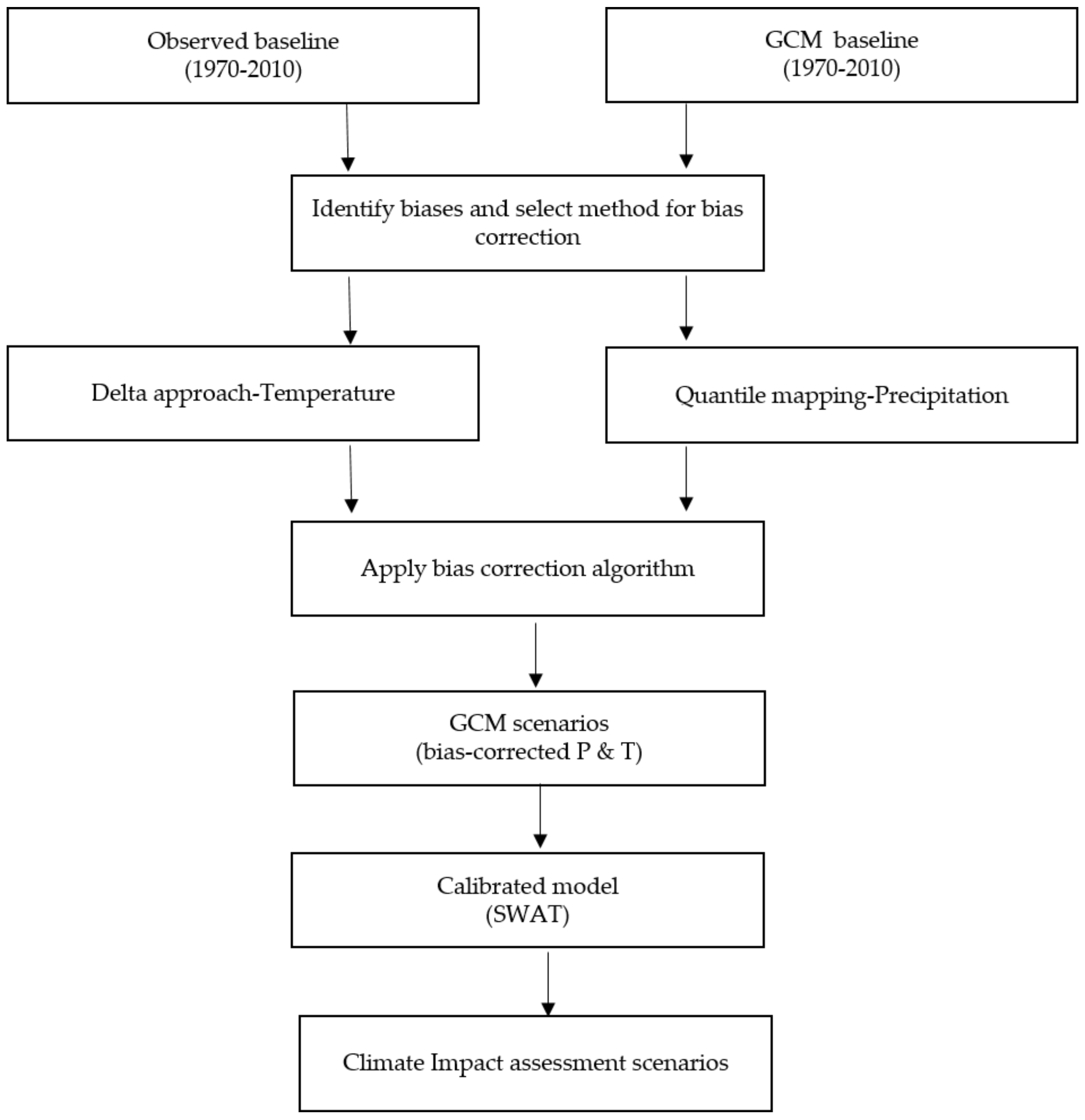
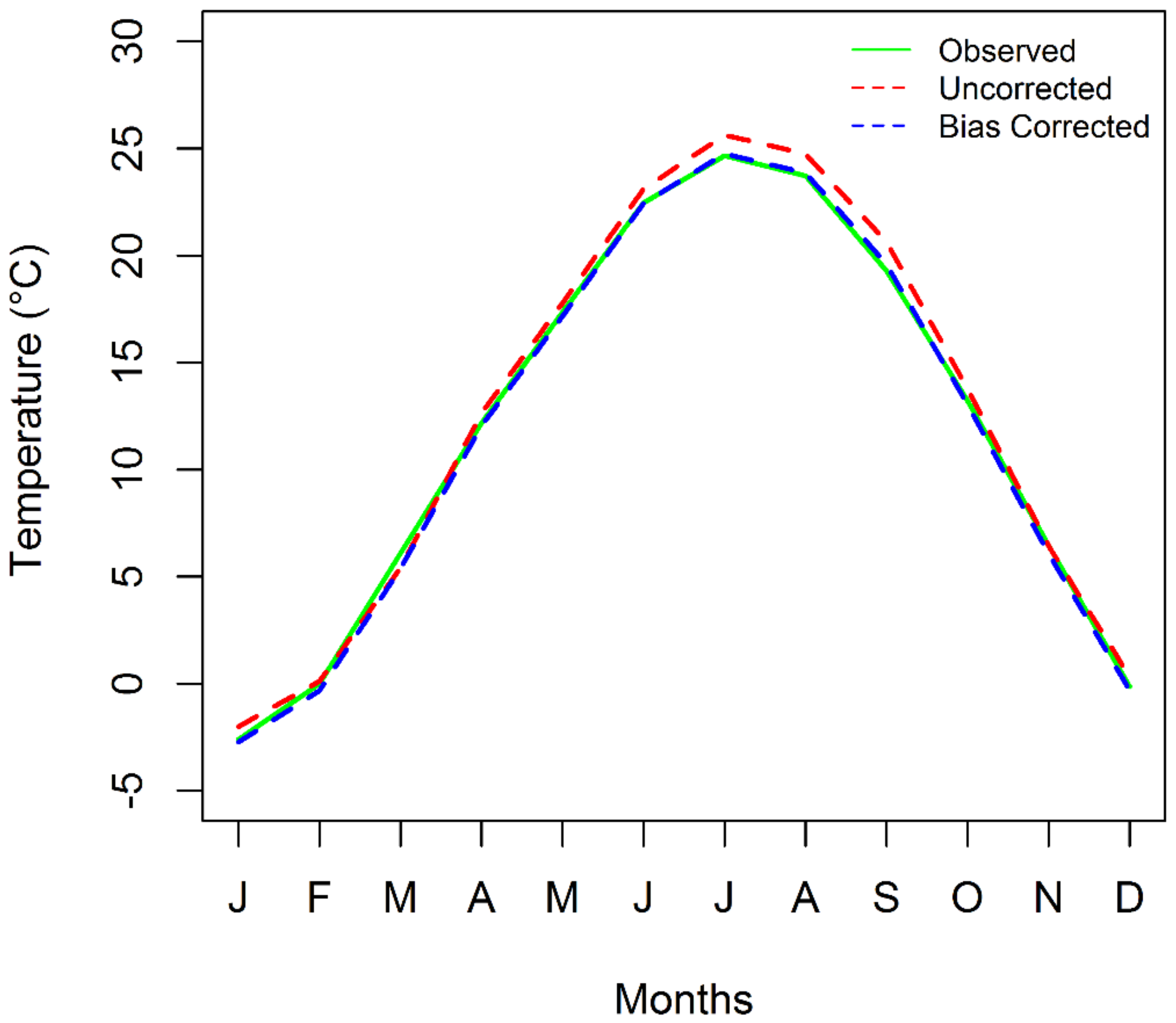
2.5. Climate Data and Bias Correction Methods

Climate projection data were obtained from the CMIP5 project [63], which provides Bias Corrected Constructed Analog (BCCA) downscaled to one-eighth degree (12 km2) from many GCM models (available at: http://gdo-dcp.ucllnl.org/downscaled_cmip_projections/) [64]. Data from twelve GCM models for four emission scenarios (RCP 2.6, RCP 4.5, RCP 6.0, and RCP 8.5) for a total of 48 unique datasets were selected for this study (Table 2 [63] and Table S1). Daily P and air T (min and max) were extracted for the four grid cells spanning the GCEW. These data were further downscaled using observed P and T data over the years 1971–2010 from the weather station located in the watershed. The bias in temperature was corrected using the delta method, and the bias in precipitation datasets was corrected using modified quantile mapping.

2.5.1. Statistical Downscaling: Temperature-Delta Method

The delta method aims to match the monthly mean of the corrected temperature values with observed temperature [73]. The correction of the temperature involves linear shifting of future temperatures using a correction factor calculated based on the difference between the historic GCM simulated and historic observed temperature data for each month [29]. Temperature data extracted from CMIP5 were corrected to correspond to the study area using the delta method. The monthly correction factor was calculated by subtracting average monthly baseline CMIP5 simulated T data and baseline observed T data (1971–2010). Daily T over the analysis period was corrected with an additive term (bj) computed for each month as Equation (1):
b j   =   C = 1 C i T i j     C = 1 C i T i j ^ C i j
where, Ci = is the total number of days for month j over the entire baseline historic period, T i j is the daily observed T in °C (maximum or minimum), and T i j ^ is the daily model temperature (maximum or minimum) on day i in month j. Finally, the additive factor for each respective month was added to raw data for bias correction (Equation (2)).
T i j   =   T i j ^   +   b j

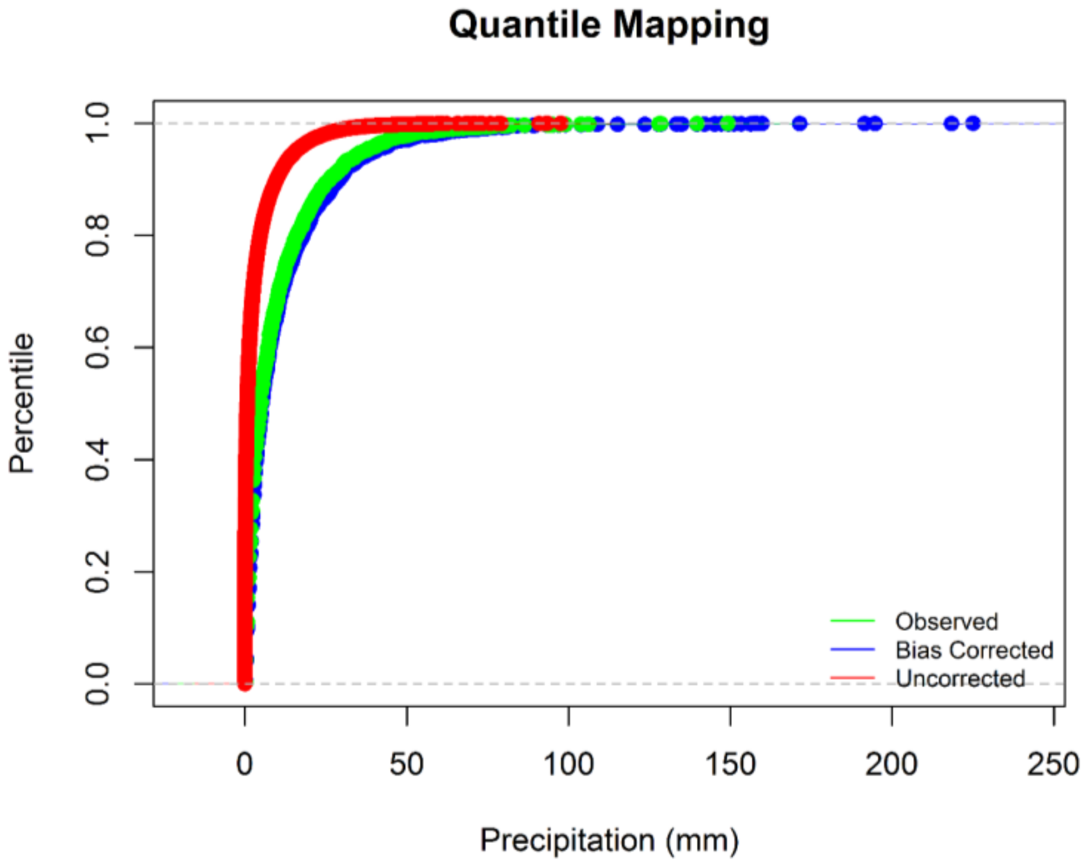
2.5.2. Statistical Downscaling: Precipitation-Quantile Mapping

Quantile mapping adjusts the daily CMIP5 precipitation values to match the statistical distribution of the observed precipitation. This method is known by many other names, for example as ‘distribution mapping’ [74,75] and ‘probability mapping’ [76,77]. One major assumption of quantile mapping is that the precipitation distribution does not change over time, and variance and skewness of the distribution remain the same with only a change in mean [78]. Cumulative Distribution Functions (CDFs) were constructed for both CMIP5 and observed daily P (1970–2010) on a monthly basis. A transfer function was constructed to transform CMIP5 data values to probabilities based on the CDF of the model distribution, and these values were transformed back to data values using the inverse CDF or quantile function of the observed distribution. This procedure is expressed mathematically as (Equation (3)):
P i , j c o r r   g c m   =   C D F o b s , j 1   [ C D F g c m , j h i s ( P i , j r a w ) ] ( P i , j r a w     P m a x , j h i s   g c m )
where, P i , j r a w , P i , j c o r r   g c m   and P m a x , j h i s   g c m are the projection’s raw CMIP5, corrected CMIP5, and maximum historical CMIP5 precipitation for i-th day of j-th month, respectively. The   C D F o b s , j 1 is the quantile function of the observed precipitation and C D F g c m , j h i s is the CDF of an individual GCM.
Quantile mapping was modified to correct two major limitations in CMIP5 P data: (1) the P frequency or dry bias, i.e., the data contain a large number of very low P days, i.e., “drizzle days”, [79] and (2) an underestimation of extreme P compared to historical observation. The number of P days was more than 300 days/year for projected gridded data compared to 94 days/year in the observed dataset (1971–2010). To correct for these excess “drizzle days”, a P threshold was determined and the P values below the threshold were removed (Equation (4)). A P threshold for each month was determined for each GCM model to ensure the same number of P days for GCM baseline and observed, as was done by Grillakis, et al. [80]. Monthly thresholds ranged from 0.60 to 4.5 mm/day; similar to ranges of P thresholds reported by Themeßl, et al. [81]. Quantile mapping was performed after removing “drizzle day” corrections.
P i , j r a w ( d )   =   { 0 ,   i f   P i , j r a w   <   P t h r e s h o l d , j P i , j r a w ,   o t h e r w i s e
The second limitation of quantile mapping is that the method limits the upper value of future daily precipitation to the highest value observed in the past. Given that climate projections indicate that precipitation events are likely to increase in magnitude and this sort of extreme event poses potential risks a second adjustment was made to the CMIP5 P data to allow a daily P to exceed the historic maximum using Equations (5) and (6). P was scaled on a monthly basis to represent the monthly extreme. A separate scaling factor was calculated for each month, where Sj is the scaling factor for a given month and P i , j h i s   g c m is the CMIP5 daily P data for month j during the historic period. This approach retained the relationship between the historic period and future periods within a CMIP5 P dataset for a given model without constraining future P data to the maximum historical observation.
P i , j c o r r   g c m   =   S j     P i , j r a w ( P i , j r a w   >   P i , j h i s   g c m )
S j   =   M a x ( P i , j o b s ) M a x ( P i , j h i s   g c m )

2.6. Simulation Scenarios. Impacts of Climate Change on Water Yield, Evapotranspiration, and Surface Runoff

The validated SWAT model was run at a daily time step starting in 1981 and continuing until 2075. For analysis, the baseline represents 1981–2010, the near future is defined as 2016–2045, and the far future is defined as 2046–2075. Different atmospheric CO2 concentrations were applied within SWAT for each RCP for different time periods; these values were calculated by averaging the projected CO2 concentrations over each 30-year period. The average was used because it is not possible to change CO2 concentration annually in SWAT. The details of CO2 concentration used for each model for each time frame and RCP are presented in Table 3. The CO2 concentration of 330 ppm was used for all the historic simulations. The ensemble median and quartile values (Q1 and Q3) of monthly water yield, evapotranspiration, and surface runoff were calculated for the three analyses periods. Reporting results as ensembles allows for greater confidence in simulated hydrological outputs [82]. Pierce, et al. [83] found that the average of a multi-model ensemble is a better predictor than any individual GCM for global studies examining the mean climate, as the ensemble of results cancels out the bias and errors.
The modified PM method was used to calculate ET. This equation allows for the incorporation of variability in radiation-use efficiency, plant growth, and transpiration induced by change in atmospheric CO2 concentration [43]. SWAT simulates the impact of change in CO2 concentration on stomatal conductance by linear interpolation between current conditions and a 40% decrease of stomatal conductance for doubling of CO2 up to 660 ppm [43]. However, SWAT does not simulate effects of CO2 on leaf area index; thus, this study does not incorporate the impact of increased CO2 concentration on leaf area.

3. Results and Discussion

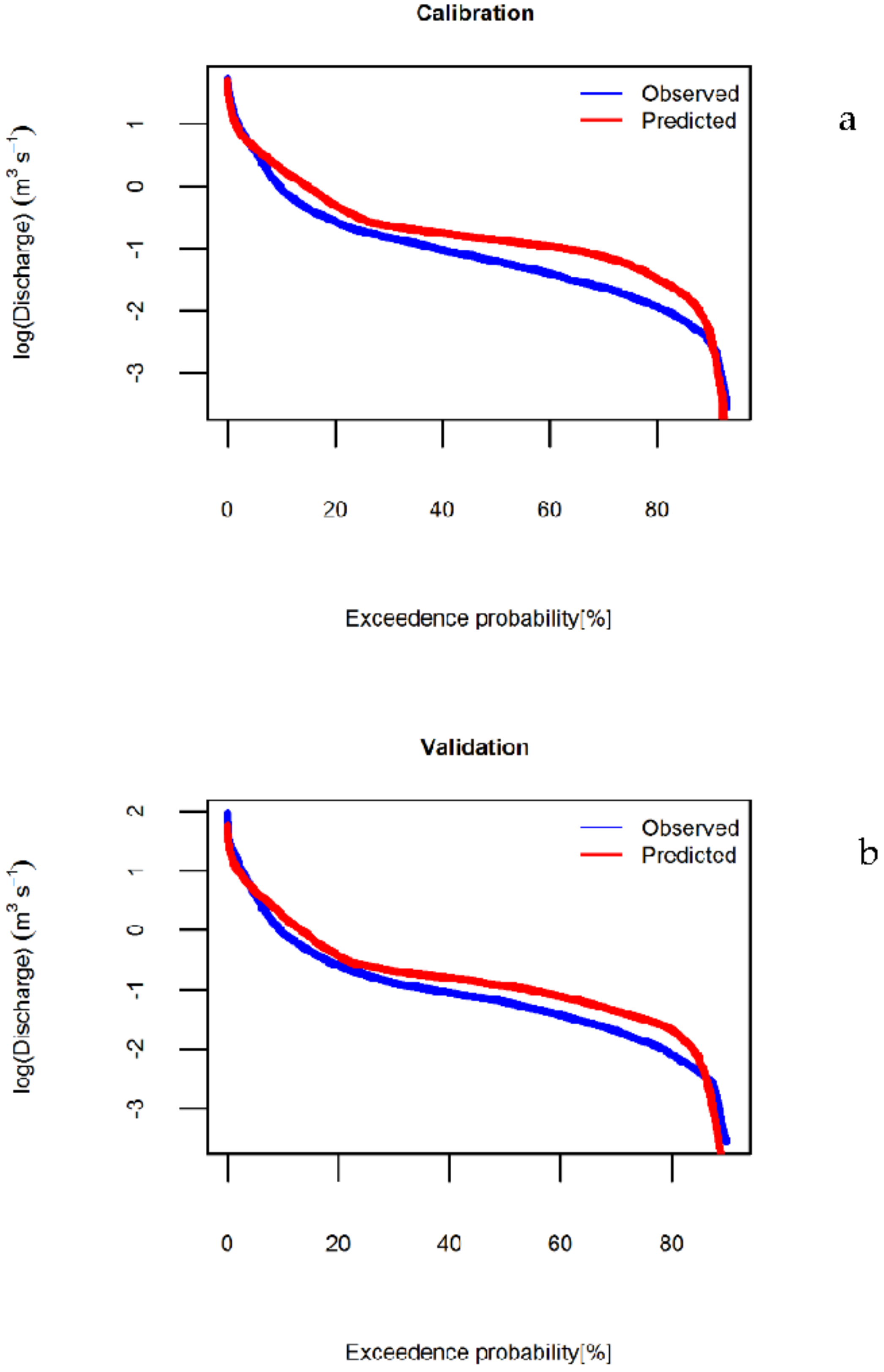
3.1. Model Calibration and Validation

The default and adjusted model parameter values are presented in Table 4. The model parameters controlling surface runoff, groundwater, and snowmelt were important parameters considered during calibration. The calibrated model parameters are similar to those reported by previous researchers for GCEW [44]. Daily streamflow simulation at weir1 (watershed outlet) resulted in r2 of 0.66, NSE of 0.66, and p-bias of 5.6% during calibration (1993–2001), and r2 of 0.60, NSE of 0.59, and p-bias of −6.9% during the validation. The model was further validated using the streamflow data at weir11 resulting in r2 of 0.73, NSE of 0.68, and p-bias of 18%. SWAT simulated dry (2007) and wet (2008) years accurately, indicating that the model was suitable for evaluating climate change impacts. The flow duration curve is a description of the frequency at which a given discharge is reached or exceeded over the simulation period. The flow duration curves for observed and simulated flow for calibration and validation periods are presented in Figure 3. The calibration objective was to superimpose observed and simulated flow duration curves to match low, intermediate, and high flow.

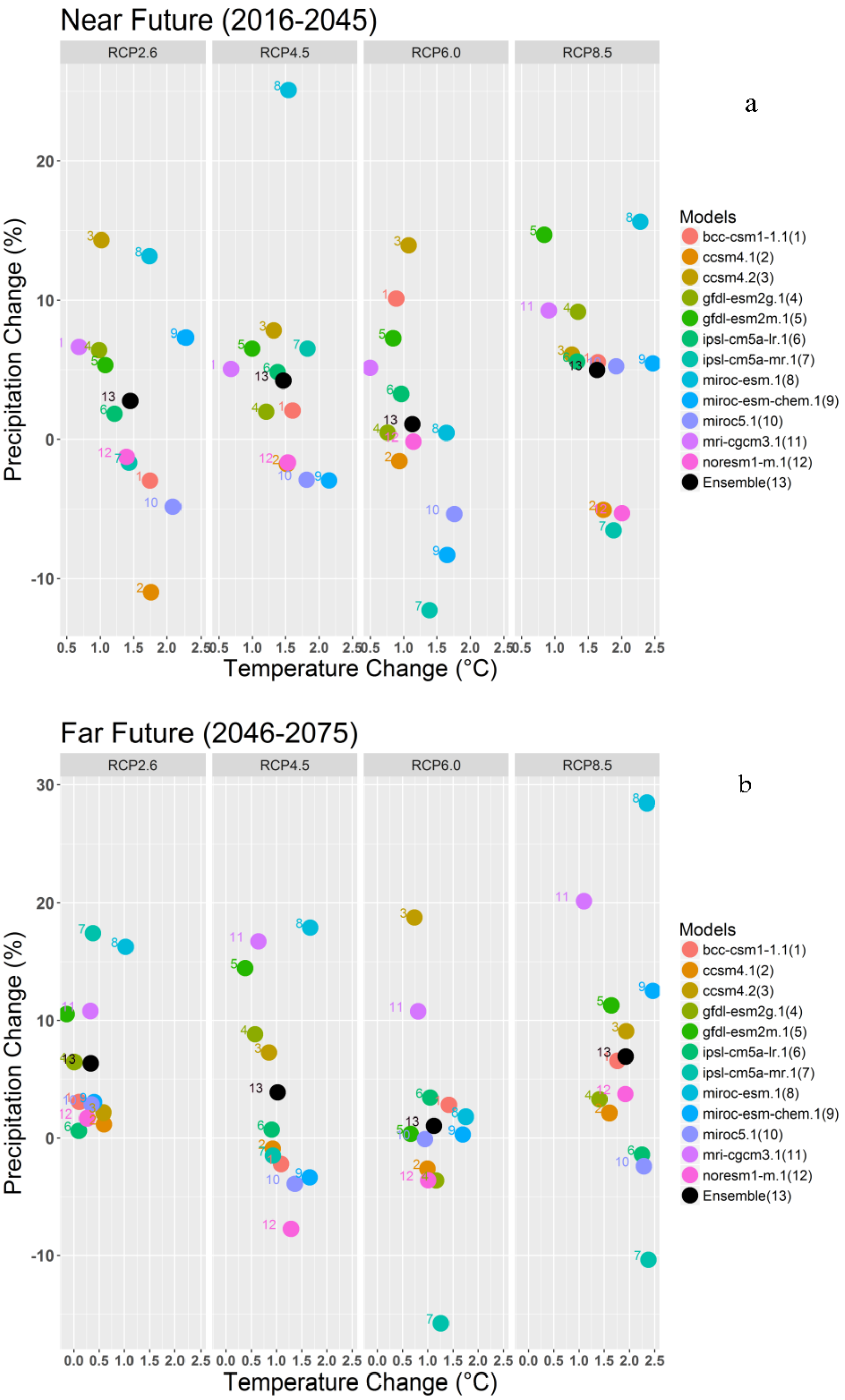
3.2. Downscaled GCM Projection

3.2.1. Temperature

Minimum temperatures were under-predicted and maximum temperatures, particularly in the summer months, were over-predicted in CMIP5 output, compared to historical observations. The scaling factors used for correction of the maximum and minimum daily T are presented in supplement Tables S2 and S3. The maximum bias was for the month of March for both the maximum and minimum T. Average monthly T (observed, CMIP5, bias-corrected) for the period 1981–2010 for one of the GCM models included in the study is presented in Figure 4 as an example. These results are consistent with previous reports of over-prediction of annual mean T for CMIP5 GCMs for Northern Eurasia [85,86], Northern hemisphere [87], and globally [88].
Figure 5 shows GCM projected changes in average annual T, between the baseline (1981–2010) and near (2016–2045) (Figure 5a) and far future (2046–2075) (Figure 5b) for the 12 sets of downscaled T data from CMIP5 for four RCP scenarios. Ensemble average T change in the near future period shows minimum T change for RCP 6.0 (1.13 °C) and maximum T change for RCP 8.5 (1.63 °C). The far future period shows minimum T change for RCP 2.6 (0.33 °C) and maximum T change for RCP 8.5 (1.92 °C). The most significant increase in T occurred for models under RCP 8.5 scenarios for both near and far future (Figure 5a,b). This is consistent with the assumptions associated with technological and socioeconomic conditions leading to the concentrations of GHGs associated with each RCP. That is, RCP 2.6 includes a decrease in the concentration of GHGs in the atmosphere to below currently observed levels, while RCP 8.5 represents the largest increases of GHG concentrations in the atmosphere. For RCP 4.5, atmospheric CO2 peaks around 2040, then declines compared to RCP 6.0, where CO2 peaks in 2080 and declines [89]. Therefore, in the near future, RCP 6.0 has the lowest CO2 concentration compared to RCP 4.5 scenarios resulting in the least T change (Figure 5a). The spread of predicted changes in T for models in RCP 4.5 (0.7 °C–2.2 °C) and RCP 8.5 (0.9 °C–2.5 °C) demonstrates the value of a multiple model ensemble approach for future climate change impact assessment studies.

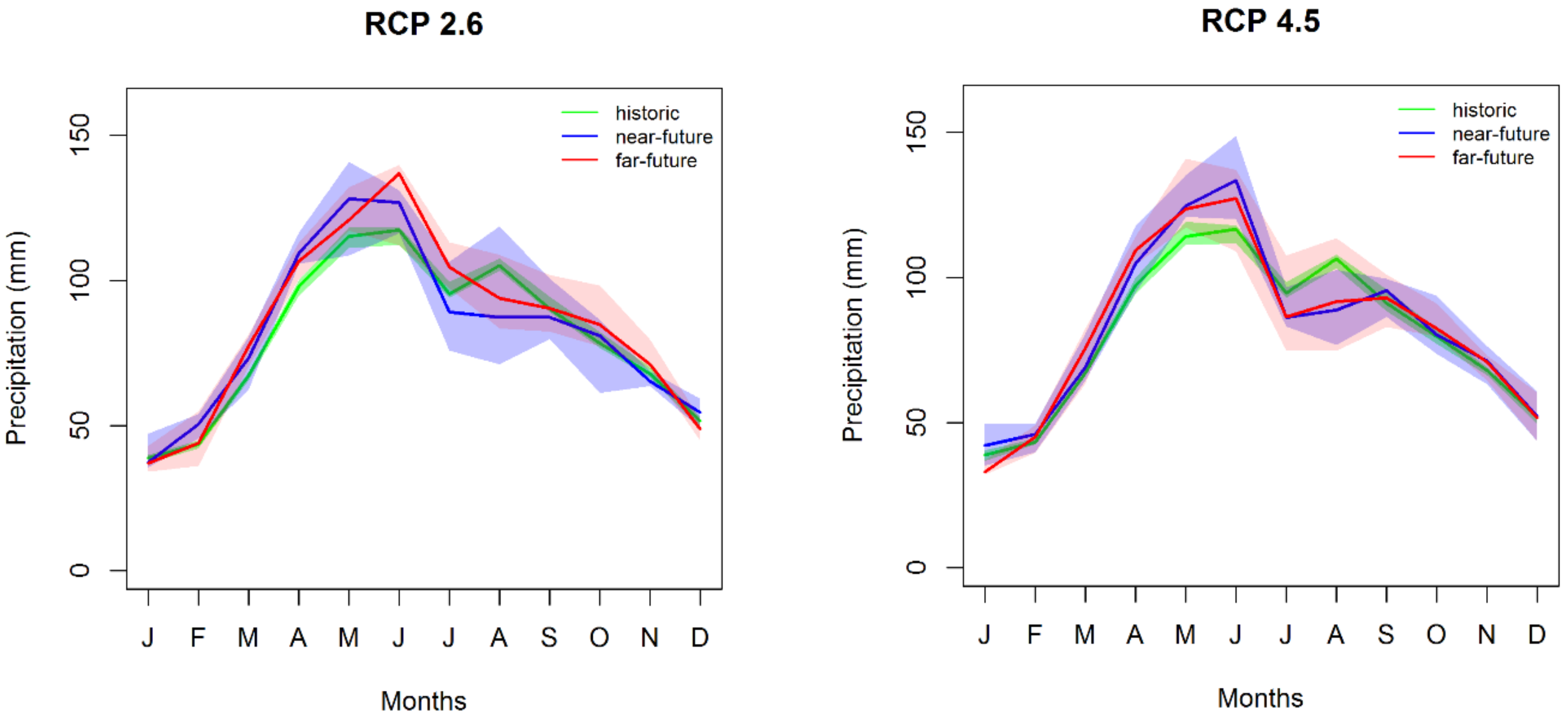
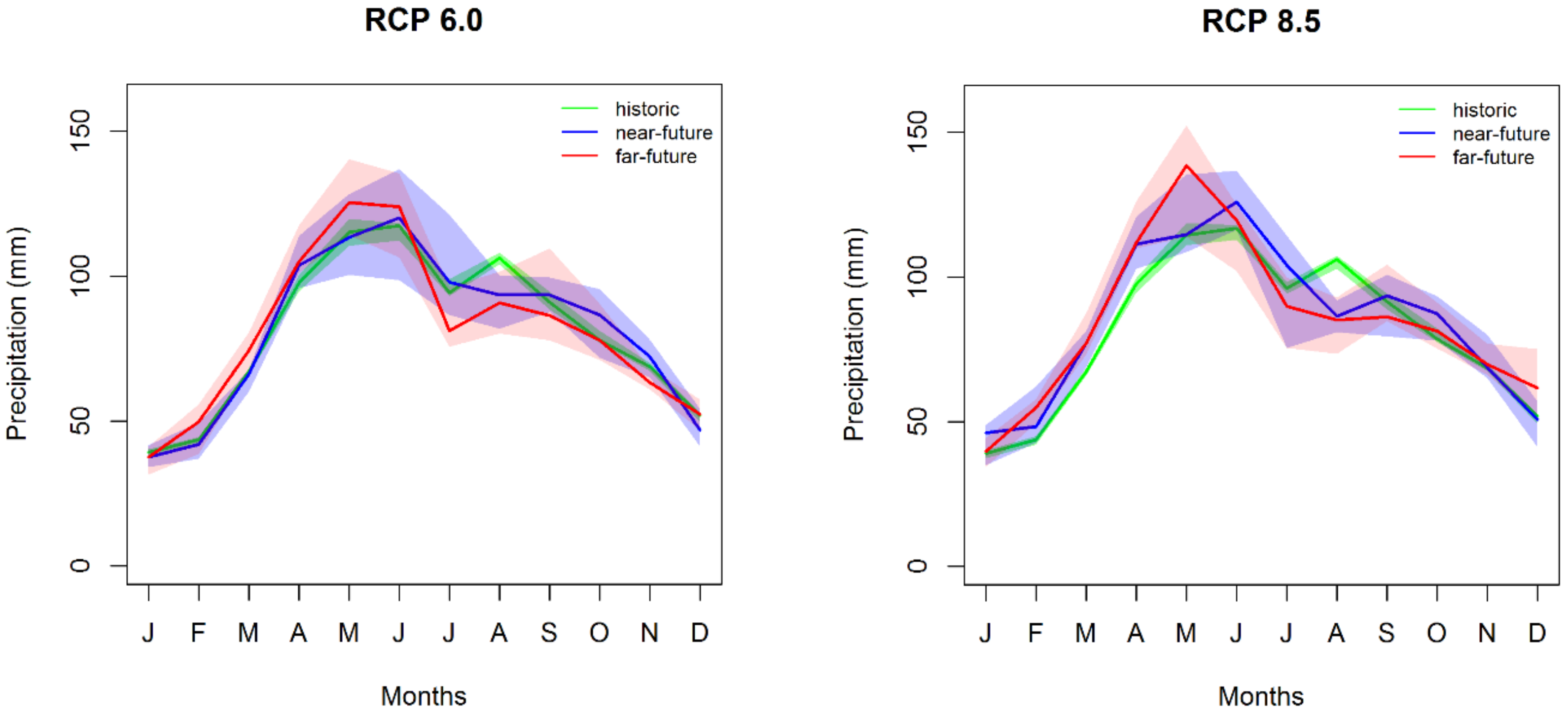
3.2.2. Precipitation

Figure 5 also shows GCM projected percentage changes in average annual P, for baseline (1981–2010), near future (2016–2045), and far future (2046–2075) respectively, for the 12 different GCMs used in this study. An ensemble P change for the far future scenario was the least for the RCP 6.0 scenario (1.0% increase) and most for RCP 8.5 (6.9% increase). The highest simulated increase in average annual precipitation was for RCP 8.5 with a change in P ranging from −7% to 16% across 12 GCMs in the near future and −10% to 28% in the far future, followed by the RCP 4.5. Note that in near future (2016–2045), RCP 4.5 had a higher CO2 concentration than RCP 6.0 [90], which may explain the elevated T and P for RCP 4.5 compared to RCP 6.0 over this period. Use of variable monthly thresholds for daily precipitation enabled exact matching of wet days between historic modeled P to observed P, which is critical for quantile mapping. The monthly P thresholds and scaling factors used to correct these biases are presented in supplement Tables S4 and S5. Quantile mapping of the CMIP5 data to the historical data for one model under the RCP 8.5 scenario (micro-esm.1) is presented in Figure 6.
Monthly ensemble median P results indicate increased spring P compared to the baseline for both near and far future for all the emission scenarios (Figure 7). A previous study also reported an increase in precipitation during the spring months based on historic data for Central US [91]. Decrease in ensemble monthly P compared to the baseline was simulated for near-future for the months from July-November for RCP 2.6 (Figure 7). For RCP 4.5, the decrease in P for July was 7% and 14%, and August was 6% and 14%, for near and far future respectively. The decrease in precipitation for July and August was 12% and 14%, and 9% and 21% for far future of RCP 6.0 and RCP 8.5 respectively. There was minimal change in the monthly precipitation during the winter months. Occurrence of more P during spring may delay agricultural operations, and dry summers with very low P may result in short-term drought and possible crop losses. Previous regional modeling efforts using the Regional Climate Models (RCM) to assess the climate change impact on hydrology of the Mississippi River Basin indicated increased future P, as high as 21% on a mean annual basis [28]. Downscaling of P based on point scale (weather station) data is more relevant at the small watershed scale and may help to better understand how changes in P and T impact the hydrological components in the watershed.

3.3. Climate Change Impact on Hydrological Output
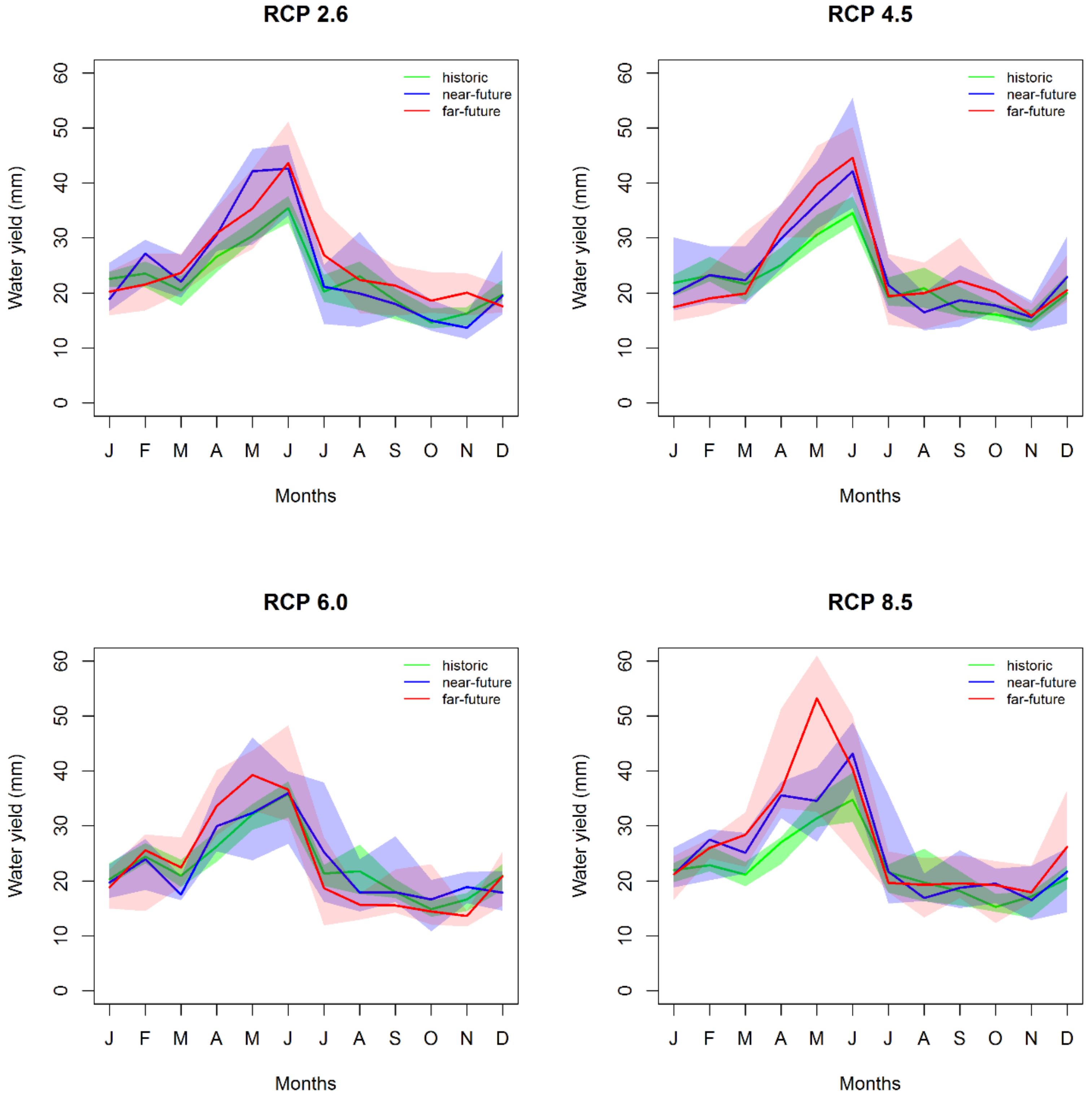
3.3.1. Water Yield

The ensemble median annual water yield was predicted to increase in both the near and far future compared to the baseline for RCP 2.6, RCP 4.5, and RCP 8.5 climate scenarios. Climate scenario RCP 6.0 showed 1% reduction in median water yield for far future scenario, due to minimum P change projected for far future for models under these climate scenarios. The highest change of 29% was observed for the far future scenario of RCP 8.5, which also resulted in the greatest increase for the near future (19%). The changes in water yield for RCP 2.6 and 4.5 were similar for near future, with the water yield increasing by around 10%. The water yield for RCP 2.6 and RCP 4.5 increased by 12% and 6% respectively, for the far future (Table 5). The models in RCP 6.0 showed very small changes in P (2% for near and 1% for far future). The increase in water yield was due to increased P; the model with the highest increase in P resulted in the highest increase in water yield. For example, the greatest increase in water yield occurred for the month of May where the P was maximum for RCP 8.5 (Figure 7 and Figure 8).
The first and third quartiles for water yield in Figure 8 show the variation in predicted water yield, which reflects the differences in GCM projections for each RCP. Despite this variation across GCM outputs, in all cases the ensemble median for near and far future was above the baseline median (Figure 8, Table 5).
For all the RCPs, the GCM ensemble range indicated a projected increase in the 3rd quartile of water yield. Monthly peak water yield occurs in June, except for the far future of RCP 6.0 and RCP 8.5 scenario where it occurs in May (Figure 8). Elevated water yield during the spring months (March, April, and May) is due to an increase in spring P projected by all four emission pathways. Such change in distribution of water yield compared to baseline may cause increase risk of extreme (flood and drought) events in the watershed. Similar trends were simulated for the region, as shown by elevated future spring and mean annual water yield for the Missouri River Basin simulated using the GCM output and the SWAT model [27]. These results, as well as previous studies [92], document that the runoff processes can be amplified due to fluctuations in P, resulting in significant impacts on streamflow. Our study shows similar results: the highest increase of water yield (83%) (270.5 to 494.9 mm) was simulated using the microc-esm.1 model under RCP 8.5, with a 28% (from 969.2 to 1239 mm) increase in precipitation compared to the baseline.

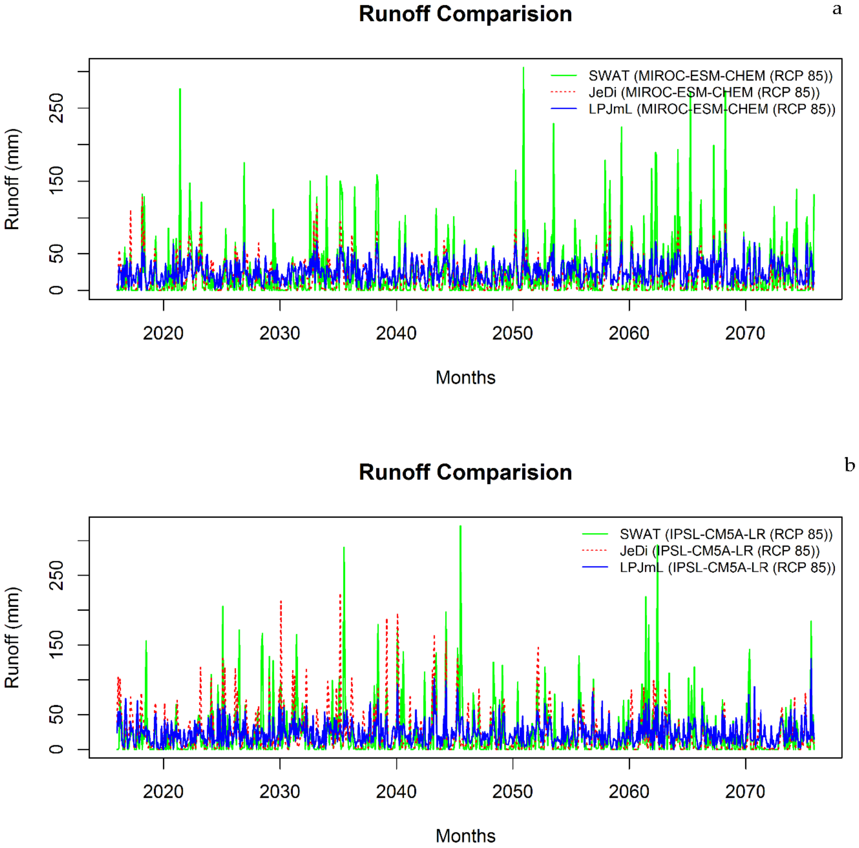
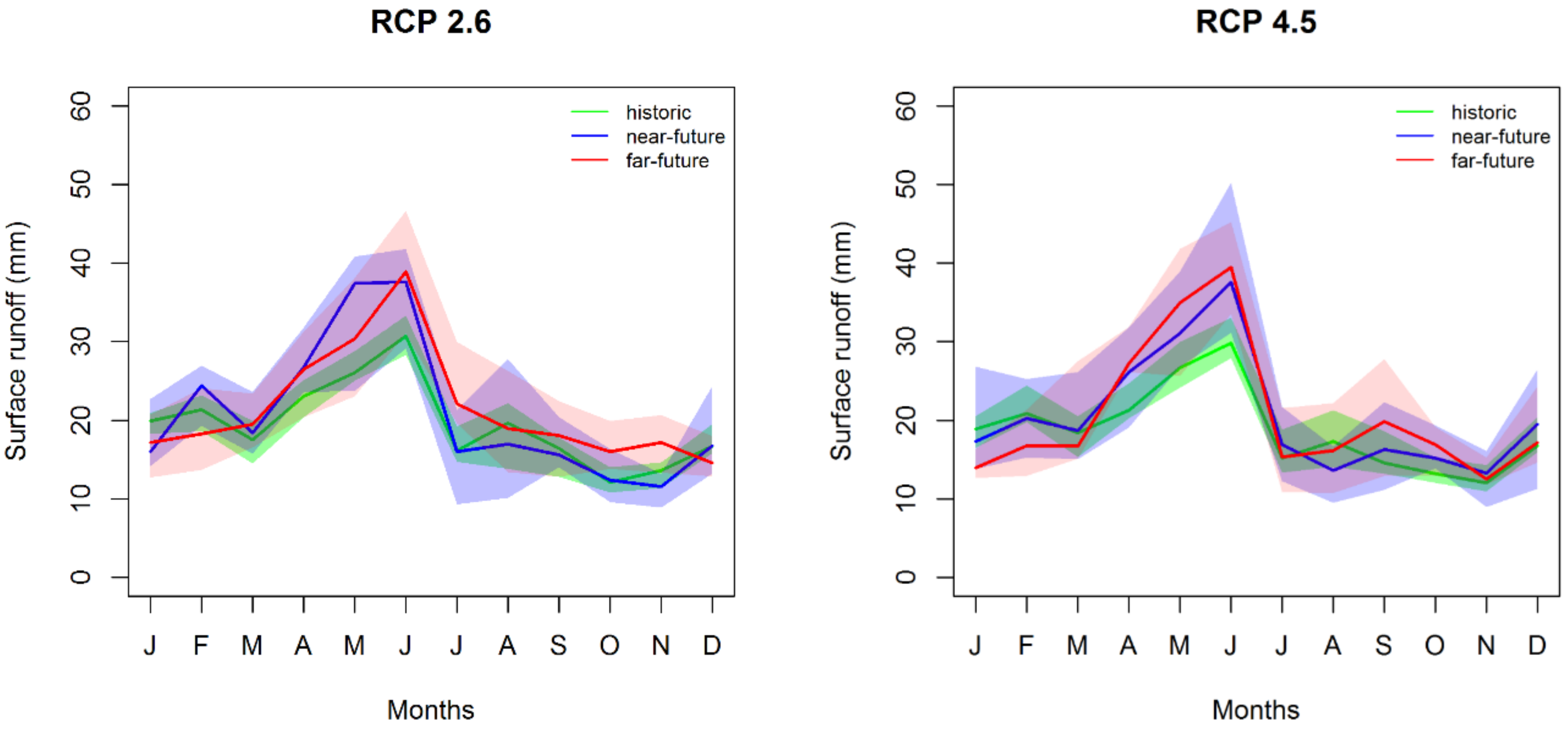
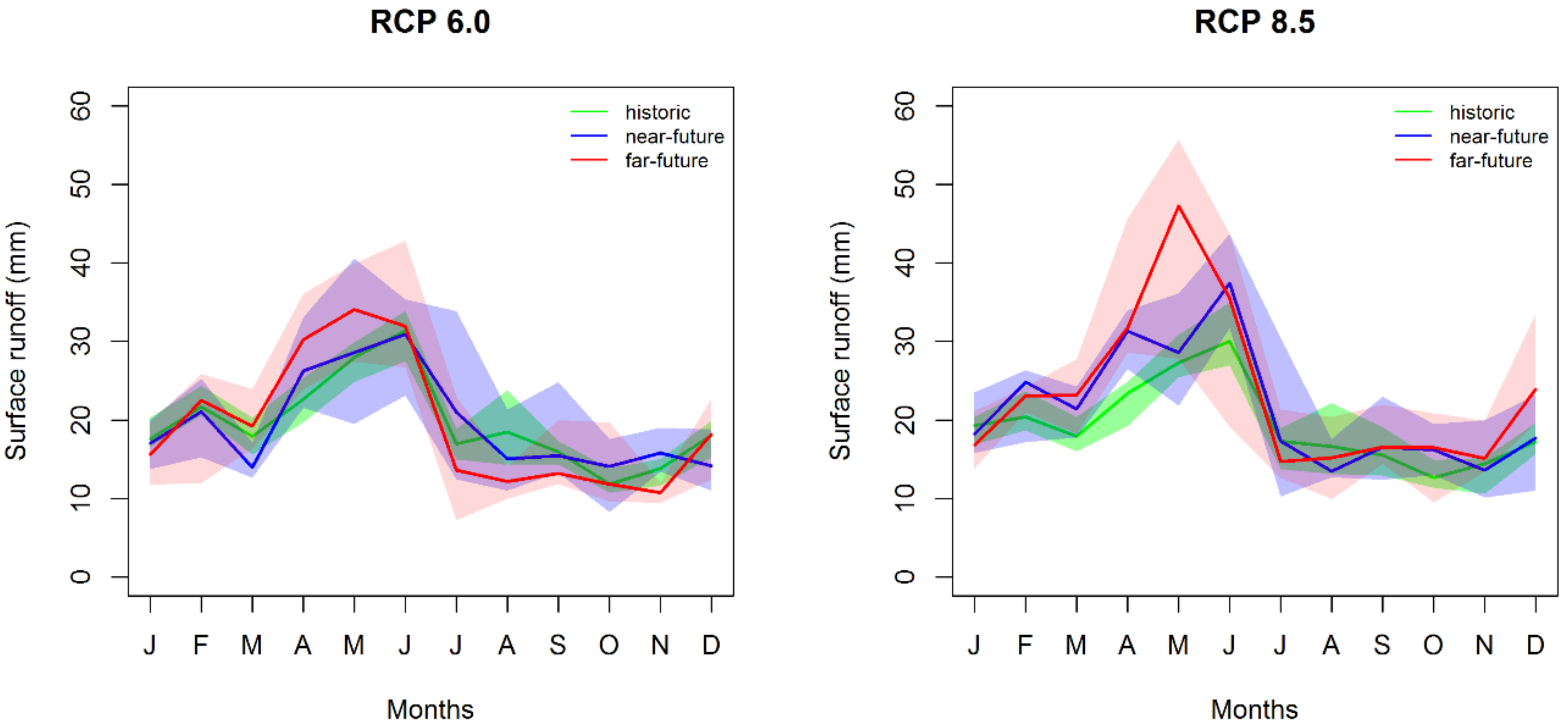
3.3.2. Surface Runoff

Ensemble mean annual surface runoff was predicted to increase compared to the historic period in all scenarios with the exception of RCP 6.0 in the far future (Figure 9). RCP 8.5 resulted in the greatest increase compared to the historic period in surface runoff for both near future (20.9%) and far future (29.9%) (Table 5). The first and the third quartile ranges for surface runoff in Figure 9 show the range in predicted runoff associated with individual climate models. These variations reflect the difference in GCM projections among RCPs (Figure 9 and Table 5). The largest increases are shown in the spring months as a direct result of increased precipitation. The monthly peak runoff occurred in June, except for in the far future of RCP 8.5, where it occurred in May (Figure 9). The magnitude of the peaks is larger than those observed in the historical dataset for all the RCPs, except RCP 6.0, which shows small change in ensemble water yield (Table 5). Decreased surface runoff in August was simulated for RCP 4.5, RCP 6.0, and RCP 8.5, compared to historic baseline (Figure 9).
The relationship between increased P and surface runoff is a function of physical characteristics of the location, e.g., soil type, land cover, and in a mathematical model is also a function of the spatial and temporal resolution of the model inputs and response. Hydrological models use geomorphologic and topographic parameters to characterize land forms to represent hydrological process [93]. The parameters used to represent the scale lead to differences in the simulated results. For example, SWAT uses detailed parameters to represent small sub-areas within a watershed, in this case 93 HRUs to represent the heterogeneity in GCEW, compared to single, spatially-averaged parameters applied in JeDi and LPJml to represent the grid that encompasses GCEW.
In this analysis, the GCM model microc-esm.1 under RCP 8.5 results in the largest increase in P, with an average annual increase of 28% (969.2 to 1239 mm), results an increase in runoff of 88% (230.6 to 434.9 mm). Jha, et al. [28] found an increased runoff of up to 51% in the Upper Mississippi River Basin (UMRB) for a 21% increase in P, using regional climate model output and SWAT. The SWAT model version used by Jha, et al. [28] was not modified to represent percolation through claypan soil. In contrast, a modified version of SWAT was used in our study to represent claypan hydrology [44]. The GCEW’s relatively larger modeled surface runoff response is likely due to increased heavy precipitation events, differences in the model spatial resolution, and accounting for the claypan condition in the watershed [44]. Lower saturated hydraulic conductivity of the claypan layer results in lower infiltration and higher runoff response. The representation of small-scale details (e.g., claypan) conditions is often overlooked in regional-scale simulations, as these models are constructed to simulate average conditions. Model correction to represent each unique local situation is not feasible in a model with a large spatial resolution. The small watershed-scale studies are important, as they help to better represent heterogeneity within the watershed, which can ultimately help local-scale decision-making.
Monthly surface runoff estimated using SWAT in GCEW was compared to the surface runoff output from the LPJmL and JeDi-DGVM models forced using two sets of CMIP5 data (miroc-esm-chem and ipsl-cm5a-lr), and obtained from ISI-MIP, Figure 10 and supplement Figures S6 and S7 [94]. For peak runoff, the flow duration curve comparison showed good agreement between SWAT and observed data (Figure 3). A lower peak value by the gridded models indicates an under-prediction of peak flow. The comparison indicates that the gridded models were unable to simulate the monthly peaks predicted by the SWAT simulations (Figure 10). Average annual surface runoff during 2016–2075 was over-predicted by 6–8% using LPJmL and under-predicted by 5–30% using JeDi-DGVM compared to the SWAT model. Paired t-test results indicate significantly lower prediction of average monthly runoff by JeDi-DVGM compared to SWAT and greater prediction by LPJmL. The results for paired t-tests are presented in Table 6.
The causes for these differences include model assumptions, model parameterization, input spatial resolution, and model structure in the respective models. Evapotranspiration was calculated using the PT method in LPJmL, compared to the PM approach in SWAT. Suleiman and Hoogenboom [95] report that the accuracy of the PM method for ET estimation is superior for predicting ET in the U.S., and that the PT method tends to overestimate ET for U.S. conditions. The difference in runoff prediction between the LPJmL and JeDi-DGVM models is also due to differences in approaches for representing dynamic vegetation in the model as presented in Section 2.3. The lower peak monthly runoff and greater low runoff values in the gridded model output may also be due to simulation at a coarse resolution with a homogenous set of parameters compared to the fine resolution input data of SWAT model (as described in Section 2.1 and Section 2.3), as well as differences in accounting for local weather (i.e., statistical downscaling) and local hydrological conditions (e.g., claypan). The comparison shows the importance of impact assessment at the smaller scale to predict hydrological change through representing soil and land use with greater detail. Recommending simulation at local scale for every single point on the globe can be resource intensive and even impossible. However, creating simulations of small watersheds that represent major characteristics of regions can be useful for anticipating risks and corresponding decision-making, especially within the agriculture sector, which can experience quick response to change in precipitation and temperature. Likewise, global gridded models, which are generally better at simulating average conditions, may be sufficient for other applications. For a global resource analyst, general trends noted by a global gridded model may be sufficient. Although LPJmL was able to represent the long-term average monthly conditions, it failed to represent extremes (peak and minimum runoff), which are important from an agricultural perspective.

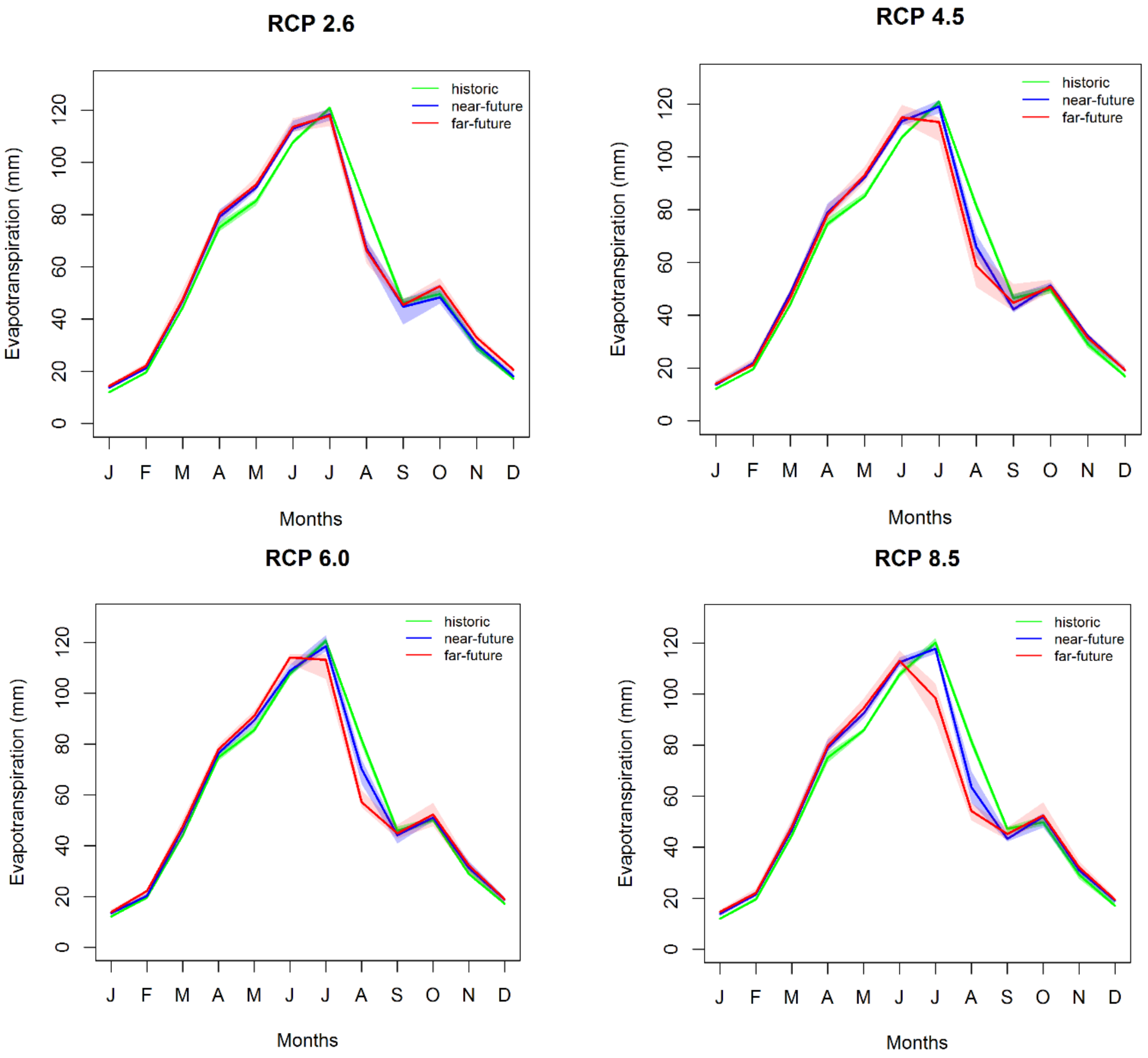
3.3.3. Evapotranspiration

Median annual ET in the near and far future had little change, −1% to 3% compared to historical observations on an annual basis (Table 5). There was minimal change in annual ET in the near future for RCP 2.6 and RCP 6.0 (Table 5). However, there was an increase in ET in spring months and a decrease in summer months for both the near and far future for all four RCPs (Figure 11). The decrease in summer ET was maximum for RCP 8.5 and minimum for RCP 2.6.
Results indicated shifts in the peak monthly ET from July (baseline) to June for RCP 4.5, RCP 6.0, and RCP 8.5 in the far future (Figure 11). Land use and land cover were fixed during the entire simulation period. Therefore, variation of the simulated ET from the watershed was mostly controlled by meteorological variables and corresponding plant growth responses. For each crop, a base T must be reached for plant growth to begin in SWAT. With increased T, base T values were reached sooner than they have been reached historically, resulting in a shift in the plant growth cycle to earlier in the calendar year. This earlier emergence of biomass resulted in a corresponding shift in evapotranspiration to earlier in the season, with an earlier peak for all far future RCPs except for 2.6. The impact of elevated T on the hydrological cycle due to shift of the crop growth cycle has been documented previously by Ficklin, et al. [96]. However, it remains unclear whether farmers would actually plant crops earlier. In addition, for this study region, increased spring precipitation may preclude early planting.

4. Conclusions

A calibrated and validated SWAT model for the GCEW was used to simulate the effect of climate change using downscaled T and P data from 12 GCMs under four emission scenarios. Downscaled climate model projections suggested an increase in spring precipitation and increased temperatures in the future for the study region, with the magnitude varying with the GCM model and emission scenarios. The change in precipitation for the extreme scenario (RCP 8.5) ranged from −7% to 16% for near future, and from −10% to 28% for far future scenarios. The majority of CMIP5 data showed a reduction of summer precipitation and increase in spring precipitation. SWAT simulated hydrological results indicated a range of possible futures due to increased temperature, precipitation changes, and elevated CO2. Results show increased water yield, surface runoff during spring months, and a shift in ET for all the RCPs except RCP 2.6 in the far future. The greatest increase in the median water yield and surface runoff (29% and 30%) compared to the baseline was for the far future of the most extreme future climate scenario, i.e., RCP 8.5. Small changes in precipitation amounts can impact the runoff and water yield response, which is especially apparent at the small watershed scale. The shift in the peak ET from July to June for RCP 4.5, RCP 6.0, and RCP 8.5 indicated the probable impact of increased CO2 concentration and temperature on planting dates and seasonality, which may ultimately impact future crop yields. Of particular concern for this watershed is the increase in precipitation, and the potential for more frequent occurrence of high-intensity rainfall events in the springtime. This could negate potential for earlier planting, noted by some researchers as a potential benefit of increasing temperatures due to climate change. Further, this study has found that cumulative precipitation is likely to decrease in the late summer; this, combined with higher temperatures, could lead to drought conditions in July and August. Depending on planting date, this could overlap with the tasseling stage of corn development. Modeling at this scale allows for a finer understanding of the patterns and processes of the hydrological response, as well as of the potential implications with regard to agricultural activity, to changes in temperature and precipitation.
The comparison with gridded model output indicated that hydrological modeling at larger scales fails to capture peak and minimum runoff, which may be very important for adaptation responses at local scales. Average annual surface runoff during 2016–2075 was over-predicted by 6–8% using LPJmL and under-predicted by 5–30% using JeDi-DGVM, compared to the SWAT model. Global gridded data with coarse spatial resolution does not capture small-scale details that are necessary for agricultural management decisions. Simulation using higher spatial resolution, as well as additional downscaling of weather data provided by CMIP5, helps to adequately represent the hydrological components of small watersheds. This may be particularly important in watersheds with problematic soils, such as claypan soils found in GCEW and the surrounding region, which have a very thin top-soil layer above a claypan to hold and supply water to plants.

Supplementary Materials

The following are available online at https://www.mdpi.com/2073-4441/10/5/564/s1, Table S1. List of the model used for impact assessment, Table S2. Monthly additive factor used for the bias correction of maximum temperature using delta method for all the models, Table S3. Monthly additive factor used for the bias correction of minimum temperature using delta method for all the models, Table S4. Monthly scaling factor used for the bias correction of precipitation using quantile mapping for gage25 datasets for all the models, Table S5. Monthly precipitation threshold (mm) used for the bias correction of precipitation using quantile mapping for gage25 datasets for all models, Figure S6. Runoff comparison simulated monthly runoff from simulation forced with MIROC-ESM-CHEM for near future (a) and far future (b) for RCP 8.5 climate scenarios for the SWAT, LPJmL and JeDi-DGVM model and, Figure S7. Runoff comparison of simulated monthly runoff from simulation forced with IPSL-CM5A-LR for near future (a) and far future (b) for RCP 8.5 climate scenarios for the SWAT, LPJmL and JeDi-DGVM model.

Author Contributions

In this article, Sagar Gautam and Christine Costello designed the study and wrote the initial draft of the manuscript and facilitated integration of team comments and revisions; Claire Baffaut contributed in the hydrological model setup and execution; Bohumil M. Svoma and Quang A. Phung contributed in statistical downscaling; Claire Baffaut, Allen Thompson and Edward J. Sadler contributed with discussions and scientific advice pertaining to hydrological processes and the functioning of the Goodwater Creek Experimental Watershed.

Funding

This research was supported by the USDA-ARS under Specific Cooperative Agreement 58-3622-4-021. ‘Climate Change Impacts on Hydrology and Productivity in Goodwater Creek Experimental Watershed’.

Acknowledgments

All Authors would like to thanks the US Department of Agriculture (USDA)-ARS, Columbia, Missouri personnel for providing the hydrology data, and watershed information for this study. We also thank the three anonymous reviewers for their comments, which greatly improved the manuscript. Costello would also like to acknowledge the team associated with the NSF RIPS project #1441131, while this grant did not provide funding for this work, discussions associated with that project inspired the comparison with global gridded model output.

Conflicts of Interest

The authors declare no conflict of interest.

References

  1. De Wit, M.; Stankiewicz, J. Changes in Surface Water Supply across Africa with Predicted Climate Change. Science 2006, 311, 1917–1921. [Google Scholar] [CrossRef] [PubMed]
  2. Schewe, J.; Heinke, J.; Gerten, D.; Haddeland, I.; Arnell, N.W.; Clark, D.B.; Dankers, R.; Eisner, S.; Fekete, B.M.; Colón-González, F.J. Multimodel Assessment of Water Scarcity under Climate Change. Proc. Natl. Acad. Sci. USA 2014, 111, 3245–3250. [Google Scholar] [CrossRef] [PubMed] [Green Version]
  3. Gregory, R.D.; Willis, S.G.; Jiguet, F.; Voříšek, P.; Klvaňová, A.; Strien, A.V.; Huntley, B.; Collingham, Y.C.; Couvet, D.; Green, R.E. An Indicator of the Impact of Climatic Change on European Bird Populations. PLoS ONE 2009, 4, e4678. [Google Scholar] [CrossRef] [PubMed] [Green Version]
  4. Moritz, C.; Agudo, R. The future of species under climate change: Resilience or decline? Science 2013, 341, 504–508. [Google Scholar] [CrossRef] [PubMed]
  5. Bellard, C.; Bertelsmeier, C.; Leadley, P.; Thuiller, W.; Courchamp, F. Impacts of climate change on the future of biodiversity. Ecol. Lett. 2012, 15, 365–377. [Google Scholar] [CrossRef] [PubMed]
  6. Walther, G.-R.; Post, E.; Convey, P.; Menzel, A.; Parmesan, C.; Beebee, T.J.C.; Fromentin, J.-M.; Hoegh-Guldberg, O.; Bairlein, F. Ecological Responses to Recent Climate Change. Nature 2002, 416, 389–395. [Google Scholar] [CrossRef] [PubMed]
  7. Schlenker, W.; Hanemann, W.M.; Fisher, A.C. The Impact of Global Warming on US Agriculture: An Econometric Analysis of Optimal Growing Conditions. Rev. Econ. Stat. 2006, 88, 113–125. [Google Scholar]
  8. Cubasch, U.; Wuebbles, D.; Chen, D.; Facchini, M.C.; Frame, D.; Mahowald, N.; Winther, J.G. Introduction: The Physical Science Basis. In Contribution of Working Group I to the Fifth Assessment Report of the Intergovernmental Panel on Climate Change; Stocker, T.F., Qin, D., Plattner, G.-K., Tignor, M., Allen, S.K., Boschung, J., Nauels, A., Xia, Y., Bex, V., Midgley, P.M., Eds.; Cambridge University Press: Cambridge, UK, 2013. [Google Scholar]
  9. Pachauri, R.K.; Allen, M.; Barros, V.; Broome, J.; Cramer, W.; Christ, R.; Church, J.; Clarke, L.; Dahe, Q.; Dasgupta, P. Climate Change 2014: Synthesis Report: Contribution of Working Groups I, II and III to the Fifth Assessment Report of the Intergovernmental Panel on Climate Change; IPCC: Geneva, Switzerland, 2014. [Google Scholar]
  10. Intergovernmental Panel on Climate Change (IPCC). Climate Change 2014: Mitigation of Climate Change; Cambridge University Press: Cambridge, UK; New York, NY, USA, 2014. [Google Scholar]
  11. Piao, S.; Ciais, P.; Huang, Y.; Shen, Z.; Peng, S.; Li, J.; Zhou, L.; Liu, H.; Ma, Y.; Ding, Y. The Impacts of Climate Change on Water Resources and Agriculture in China. Nature 2010, 467, 43–51. [Google Scholar] [CrossRef] [PubMed]
  12. Kucharik, C.J.; Serbin, S.P. Impacts of Recent Climate Change on Wisconsin Corn and Soybean Yield Trends. Environ. Res. Lett. 2008, 3, 034003. [Google Scholar] [CrossRef]
  13. Le, P.V.; Kumar, P.; Drewry, D.T. Implications for the Hydrologic Cycle Under Climate Change due to the Expansion of Bioenergy Crops in the Midwestern United States. Proc. Natl. Acad. Sci. USA 2011, 108, 15085–15090. [Google Scholar] [CrossRef] [PubMed]
  14. Intergovernmental Panel on Climate Change (IPCC). What Is a GCM? Available online: http://www.ipcc-data.org/guidelines/pages/gcm_guide.html (accessed on 11 September 2017).
  15. Taylor, K.E.; Stouffer, R.J.; Meehl, G.A. An Overview of CMIP5 and the Experiment Design. Bull. Am. Meteorol. Soc. 2012, 93, 485–498. [Google Scholar] [CrossRef]
  16. Schneider, S.H. Introduction to climate modeling. In Coupled Climate System Modeling; Trenberth, K.E., Ed.; Cambridge University Press: Cambridge, UK, 1992. [Google Scholar]
  17. Peel, M.C.; Srikanthan, R.; McMahon, T.A.; Karoly, D.J. Uncertainty in runoff based on Global Climate Model precipitation and temperature data & ndash; Part 2: Estimation and uncertainty of annual runoff and reservoir yield. Hydrol. Earth Syst. Sci. Discuss. 2014, 11, 4579–4638. [Google Scholar]
  18. Qiao, L.; Pan, Z.; Herrmann, R.B.; Hong, Y. Hydrological Variability and Uncertainty of Lower Missouri River Basin Under Changing Climate. JAWRA J. Am. Water Resour. Assoc. 2014, 50, 246–260. [Google Scholar] [CrossRef]
  19. Fowler, H.; Blenkinsop, S.; Tebaldi, C. Linking Climate Change Modelling to Impacts Studies: Recent Advances in Downscaling Techniques for Hydrological Modelling. Int. J. Climatol. 2007, 27, 1547–1578. [Google Scholar] [CrossRef]
  20. Haasnoot, M.; van Deursen, W.P.A.; Guillaume, J.H.A.; Kwakkel, J.H.; van Beek, E.; Middelkoop, H. Fit For Purpose? Building and Evaluating a Fast, Integrated Model for Exploring Water Policy Pathways. Environ. Model. Softw. 2014, 60, 99–120. [Google Scholar] [CrossRef]
  21. Jha, M.; Gassman, P.; Panagopoulos, Y. Regional Changes in Nitrate Loadings in the Upper Mississippi River Basin under Predicted Mid-century Climate. Reg. Environ. Chang. 2015, 15, 449–460. [Google Scholar] [CrossRef]
  22. Panagopoulos, Y.; Gassman, P.; Arritt, R.; Herzmann, D.; Campbell, T.; Jha, M.; Kling, C.; Srinivasan, R.; White, M.; Arnold, J. Surface Water Quality and Cropping Systems Sustainability Under a Changing Climate in the Upper Mississippi River Basin. J. Soil Water Conserv. 2014, 69, 483–494. [Google Scholar] [CrossRef]
  23. Ouyang, F.; Zhu, Y.; Fu, G.; Lü, H.; Zhang, A.; Yu, Z.; Chen, X. Impacts of Climate Change Under CMIP5 RCP Scenarios on Streamflow in the Huangnizhuang Catchment. Stoch. Environ. Res. Risk Assess. 2015, 29, 1781–1795. [Google Scholar] [CrossRef]
  24. Ficklin, D.; Stewart, I.; Maurer, E. Effects of Projected Climate Change on the Hydrology in the Mono Lake Basin, California. Clim. Chang. 2013, 116, 111–131. [Google Scholar] [CrossRef]
  25. Ficklin, D.L.; Stewart, I.T.; Maurer, E.P. Climate Change Impacts on Streamflow and Subbasin-Scale Hydrology in the Upper Colorado River Basin. PLoS ONE 2013, 8, e71297. [Google Scholar] [CrossRef] [PubMed]
  26. Mohammed, I.N.; Bomblies, A.; Wemple, B.C. The Use of CMIP5 Data to Simulate Climate Change Impacts on Flow Regime within the Lake Champlain Basin. J. Hydrol. Reg. Stud. 2015, 3, 160–186. [Google Scholar] [CrossRef]
  27. Stone, M.C.; Hotchkiss, R.H.; Mearns, L.O. Water Yield Responses to High and Low Spatial Resolution Climate Change Scenarios in the Missouri River Basin. Geophys. Res. Lett. 2003, 30, 1186. [Google Scholar] [CrossRef]
  28. Jha, M.; Pan, Z.; Takle, E.S.; Gu, R. Impacts of Climate Change on Streamflow in the Upper Mississippi River Basin: A Regional Climate Model Perspective. J. Geophys. Res. Atmos. 2004, 109, 09105. [Google Scholar] [CrossRef]
  29. Choi, W.; Pan, F.; Wu, C. Impacts of climate change and urban growth on the streamflow of the Milwaukee River (Wisconsin, USA). Reg. Environ. Chang. 2017, 17, 889–899. [Google Scholar] [CrossRef]
  30. Tavakoli, M.; De Smedt, F. Impact of climate change on streamflow and soil moisture in the Vermilion Basin, Illinois. J. Hydrol. Eng. 2011, 17, 1059–1070. [Google Scholar] [CrossRef]
  31. Jha, M.K.; Gassman, P.W. Changes in hydrology and streamflow as predicted by a modelling experiment forced with climate models. Hydrol. Process. 2014, 28, 2772–2781. [Google Scholar] [CrossRef]
  32. Ahmadi, M.; Records, R.; Arabi, M. Impact of Climate Change on Diffuse Pollutant Fluxes at the Watershed Scale. Hydrol. Process. 2014, 28, 1962–1972. [Google Scholar] [CrossRef]
  33. Al-Mukhtar, M.; Dunger, V.; Merkel, B. Assessing the Impacts of Climate Change on Hydrology of the Upper Reach of the Spree River: Germany. Water Resour. Manag. 2014, 28, 2731–2749. [Google Scholar] [CrossRef]
  34. Ye, L.; Grimm, N. Modelling Potential Impacts of Climate Change on Water and Nitrate Export from a Mid-sized, Semiarid Watershed in the US Southwest. Clim. Chang. 2013, 120, 419–431. [Google Scholar] [CrossRef]
  35. Seaber, P.R.; Kapinos, F.P.; Knapp, G.L. Hydrologic Unit Maps; USGPO: Washington, DC, USA, 1987. [Google Scholar]
  36. Liang, X. A Two-Layer Variable Infiltration Capacity Land Surface Representation for General Circulation Models; NASA: Washington, DC, USA, 1994. [Google Scholar]
  37. Williams, J.R.; Izaurralde, R.C. The APEX model. In Watershed Models; Singh, V.P., Frevert, D.K., Eds.; CRC Press, Taylor & Francis: Boca Raton, FL, USA, 2006. [Google Scholar]
  38. Freeze, R.A.; Harlan, R. Blueprint for a Physically-based, Digitally-simulated Hydrologic Response Model. J. Hydrol. 1969, 9, 237–258. [Google Scholar] [CrossRef]
  39. Clark, M.P.; Bierkens, M.F.P.; Samaniego, L.; Woods, R.A.; Uijenhoet, R.; Bennet, K.E.; Pauwels, V.R.N.; Cai, X.; Wood, A.W.; Peters-Lidard, C.D. The Evolution of Process-based Hydrologic Models: Historical Challenges and the Collective Quest for Physical Realism. Hydrol. Earth Syst. Sci. Discuss. 2017, 2017, 1–14. [Google Scholar]
  40. Sadler, E.J.; Lerch, R.N.; Kitchen, N.R.; Anderson, S.H.; Baffaut, C.; Sudduth, K.A.; Prato, A.A.; Kremer, R.J.; Vories, E.D.; Myers, D.B. Long-term Agroecosystem Research in the Central Mississippi River Basin: Introduction, Establishment, and Overview. J. Environ. Qual. 2015, 44, 3–12. [Google Scholar] [CrossRef] [PubMed]
  41. Arnold, J.G.; Srinivasan, R.; Muttiah, R.S.; Williams, J.R. Large Area Hydrologic Modeling and Assessment Part I: Model Development; Wiley Online Library: Hoboken, NJ, USA, 1998. [Google Scholar]
  42. Santhi, C.; Arnold, J.G.; Williams, J.R.; Dugas, W.A.; Srinivasan, R.; Hauck, L.M. Validation of the Swat Model on a Large Rwer Basin with Point and Nonpoint Sources. J. Am. Water Resour. Assoc. 2001, 37, 1169–1188. [Google Scholar] [CrossRef]
  43. Neitsch, S.L.; Arnold, J.G.; Kiniry, J.R.; Williams, J.R. Soil and Water Assessment Tool Theoretical Documentation: Version 2009; USDA Agricultural Research Service and Texas A&M Blackland Research Center: Temple, TX, USA, 2011. [Google Scholar]
  44. Baffaut, C.; John Sadler, E.; Ghidey, F.; Anderson, S.H. Long-term Agroecosystem Research in the Central Mississippi River Basin: SWAT Simulation of Flow and Water Quality in the Goodwater Creek Experimental Watershed. J. Environ. Qual. 2015, 44, 84–96. [Google Scholar] [CrossRef] [PubMed]
  45. Udawatta, R.P.; Motavalli, P.P.; Garrett, H.E. Phosphorus Loss and Runoff Characteristics in Three Adjacent Agricultural Watersheds with Claypan Soils. J. Environ. Qual. 2004, 33, 1709–1719. [Google Scholar] [CrossRef] [PubMed]
  46. Jung, W.; Kitchen, N.; Sudduth, K.; Anderson, S. Spatial Characteristics of Claypan Soil Properties in an Agricultural Field. Soil Sci. Soc. Am. J. 2006, 70, 1387–1397. [Google Scholar] [CrossRef]
  47. Sadler, E.J.; Sudduth, K.A.; Drummond, S.T.; Vories, E.D.; Guinan, P.E. Long-term Agroecosystem Research in the Central Mississippi River Basin: Goodwater Creek Experimental Watershed Weather Data. J. Environ. Qual. 2015, 44, 13–17. [Google Scholar] [CrossRef] [PubMed]
  48. Hempel, S.; Frieler, K.; Warszawski, L.; Schewe, J.; Piontek, F. A trend-preserving bias correction–the ISI-MIP approach. Earth Syst. Dyn. 2013, 4, 219–236. [Google Scholar] [CrossRef]
  49. Warszawski, L.; Frieler, K.; Huber, V.; Serdeczny, O.; Piontek, F.; Schewe, J. Research Design of the Intersectoral Impact Model Intercomparison Project (ISI-MIP). Proc. Natl. Acad. Sci. USA 2014, 111, 3228–3232. [Google Scholar] [CrossRef] [PubMed]
  50. Baffaut, C.; Sadler, E.J.; Ghidey, F. Long-term Agroecosystem Research in the Central Mississippi River Basin: Goodwater Creek experimental Watershed Flow Data. J. Environ. Qual. 2015, 44, 18–27. [Google Scholar] [CrossRef] [PubMed]
  51. Missouri Spatial Data Information Services (MSDIS), 2016. Available online: http://msdis.missouri.edu/data/dem/ (accessed on 25 April 2018).
  52. Soil Survey Geographic Data (SSURGO), 2016. Available online: http://websoilsurvey.sc.egov.usda.gov/App/WebSoilSurvey.aspx (accessed on 25 April 2018).
  53. National Agricultural Statistics Service (NASS) Cropland Data Layer (CDL), 2010. Available online: http://nassgeodata.gmu.edu/CropScape/ (accessed on 25 April 2018).
  54. Bondeau, A.; Smith, P.C.; Zaehle, S.; Schaphoff, S.; Lucht, W.; Cramer, W.; Gerten, D.; Lotze-Campen, H.; Müller, C.; Reichstein, M. Modelling the Role of Agriculture for the 20th Century Global Terrestrial Carbon Balance. Glob. Chang. Biol. 2007, 13, 679–706. [Google Scholar] [CrossRef]
  55. Pavlick, R.; Drewry, D.T.; Bohn, K.; Reu, B.; Kleidon, A. The Jena Diversity-Dynamic Global Vegetation Model (JeDi-DGVM): A Diverse Approach to Representing Terrestrial Biogeography and Biogeochemistry based on Plant functional Trade-offs. Biogeosciences 2013, 10, 4137–4177. [Google Scholar] [CrossRef]
  56. Nachtergaele, F.; van Velthuizen, H.; Verelst, L.; Batjes, N.; Dijkshoorn, J.; van Engelen, V.; Fischer, G.; Jones, A.; Montanarella, L.; Petri, M. Harmonized World Soil Database; ISRIC: Wageningen, The Netherlands, 2009. [Google Scholar]
  57. Klein Goldewijk, K. A Historical Land Use Data Set for the Holocene, HYDE 3.2; EGU General Assembly Conference Abstracts: Vienna, Austria, 2016; p. 1574. [Google Scholar]
  58. Diimenil, M.E.; Giorgetta, M.; Schlese, U.; Schullzweida, U. The Atmospheric General Circulation Model ECHAM-4: Model Description and Simulation of Present-Day Climate; MPI Report 218; Max Planck Institut Meteorologie: Hamburg, Germany, 1996. [Google Scholar]
  59. The Inter-Sectoral Impact Model Intercomparision Project (ISI-MIP) Data Repository, 2014. Available online: https://esg.pik-potsdam.de/search/isimip-ft/ (accessed on 25 April 2018).
  60. Abbaspour, K.; Vejdani, M.; Haghighat, S. SWAT-CUP Calibration and Uncertainty Programs for SWAT. In MODSIM 2007 International Congress on Modelling and Simulation; Modelling and Simulation Society of Australia and New Zealand: Canberra, Australia, 2007. [Google Scholar]
  61. Neitsch, S.; Arnold, J.; Kiniry, J.E.A.; Srinivasan, R.; Williams, J. Soil and Water Assessment Tool User’s Manual Version 2000; GSWRL Report 202; Grassland, Soil & Water Research Laboratory: Temple, TX, USA, 2002. [Google Scholar]
  62. Moriasi, D.N.; Gitau, M.W.; Pai, N.; Daggupati, P. Hydrologic and Water Quality Models: Performance Measures and Evaluation Criteria. Trans. ASABE 2015, 58, 1763–1785. [Google Scholar]
  63. Maurer, E.P.; Brekke, L.; Pruitt, T.; Duffy, P.B. Fine-resolution Climate Projections Enhance Regional Climate Change Impact Studies. Eos Trans. Am. Geophys. Union 2007, 88, 504. [Google Scholar] [CrossRef]
  64. Bias Corrected Constructed Analog (BCCA) Downscaled Data, 2014. Available online: http://gdo-dcp.ucllnl.org/downscaled_cmip_projections/ (accessed on 25 April 2018).
  65. Wu, T.; Song, L.; Li, W.; Wang, Z.; Zhang, H.; Xin, X.; Zhang, Y.; Zhang, L.; Li, J.; Wu, F.; et al. An Overview of BCC Climate System Model Development and Application for Climate Change Studies. Acta Meteorol. Sin. 2014, 28, 34–56. [Google Scholar] [CrossRef]
  66. Gent, P.R.; Danabasoglu, G.; Donner, L.J.; Holland, M.M.; Hunke, E.C.; Jayne, S.R.; Lawrence, D.M.; Neale, R.B.; Rasch, P.J.; Vertenstein, M. The Community Climate System Model Version 4. J. Clim. 2011, 24, 4973–4991. [Google Scholar] [CrossRef]
  67. Dunne, J.P.; John, J.G.; Adcroft, A.J.; Griffies, S.M.; Hallberg, R.W.; Shevliakova, E.; Stouffer, R.J.; Cooke, W.; Dunne, K.A.; Harrison, M.J. GFDL’s ESM2 Global Coupled Climate-carbon Earth System Models. Part I: Physical Formulation and Baseline Simulation Characteristics. J. Clim. 2012, 25, 6646–6665. [Google Scholar] [CrossRef]
  68. Dunne, J.P.; John, J.G.; Shevliakova, E.; Stouffer, R.J.; Krasting, J.P.; Malyshev, S.L.; Milly, P.; Sentman, L.T.; Adcroft, A.J.; Cooke, W. GFDL’s ESM2 Global Coupled Climate–Carbon Earth System Models. Part II: Carbon System Formulation and Baseline Simulation Characteristics. J. Clim. 2013, 26, 2247–2267. [Google Scholar] [CrossRef]
  69. Watanabe, S.; Hajima, T.; Sudo, K.; Nagashima, T.; Takcmura, T.; Okajima, H.; Nozawa, T.; Kawase, H.; Abe, M.; Yokohata, T. MIROC-ESM 2010: Model Description and Basic Results of CMIP5-20c3m experiments. Geosci. Model Dev. 2011, 4, 845–872. [Google Scholar] [CrossRef]
  70. Watanabe, M.; Suzuki, T.; O’ishi, R.; Komuro, Y.; Watanabe, S.; Emori, S.; Takemura, T.; Chikira, M.; Ogura, T.; Sekiguchi, M. Improved Climate Simulation by MIROC5: Mean States, Variability, and Climate Sensitivity. J. Clim. 2010, 23, 6312–6335. [Google Scholar] [CrossRef]
  71. Yukimoto, S.; Adachi, Y.; Hosaka, M.; Sakami, T.; Yoshimura, H.; Hirabara, M.; Tanaka, T.Y.; Shindo, E.; Tsujino, H.; Deushi, M. A New Global Climate Model of the Meteorological Research Institute: MRI-CGCM3-Model Description and Basic Performance. J. Meteorol. Soc. Jpn. 2012, 90, 23–64. [Google Scholar] [CrossRef]
  72. Bentsen, M.; Bethke, I.; Debernard, J.; Iversen, T.; Kirkevåg, A.; Seland, Ø.; Drange, H.; Roelandt, C.; Seierstad, I.; Hoose, C. The Norwegian Earth System Model, NorESM1-M-Part 1: Description and Basic Evaluation. Geosci. Model Dev. Discuss. 2012, 5, 2843–2931. [Google Scholar] [CrossRef]
  73. Lenderink, G.; Buishand, A.; Deursen, W.V. Estimates of Future Discharges of the River Rhine using Two Scenario Methodologies: Direct Versus Delta Approach. Hydrol. Earth Syst. Sci. 2007, 11, 1145–1159. [Google Scholar] [CrossRef]
  74. Boé, J.; Terray, L.; Habets, F.; Martin, E. Statistical and Dynamical Downscaling of the Seine Basin Climate for Hydro-Meteorological Studies. Int. J. Climatol. 2007, 27, 1643–1655. [Google Scholar] [CrossRef]
  75. Johnson, F.; Sharma, A. Accounting for Interannual Variability: A Comparison of Options for Water Resources Climate Change Impact Assessments. Water Resour. Res. 2011, 47, 04508. [Google Scholar] [CrossRef]
  76. Block, P.J.; Souza Filho, F.A.; Sun, L.; Kwon, H.H. A Streamflow Forecasting Framework using Multiple Climate and Hydrological Models; Wiley Online Library: Hoboken, NJ, USA, 2009. [Google Scholar]
  77. Ines, A.V.; Hansen, J.W. Bias Correction of Daily GCM Rainfall for Crop Simulation Studies. Agric. For. Meteorol. 2006, 138, 44–53. [Google Scholar] [CrossRef]
  78. Li, H.; Sheffield, J.; Wood, E.F. Bias Correction of Monthly Precipitation and Temperature Fields from Intergovernmental Panel on Climate Change AR4 Models using Equidistant Quantile Matching. J. Geophys. Res. Atmos. 2010, 115, 1984–2012. [Google Scholar] [CrossRef]
  79. Hidalgo, H.G.; Dettinger, M.D.; Cayan, D.R. Downscaling with Constructed Analogues: Daily Precipitation and Temperature Fields Over the United States; California Energy Commission: Sacramento, CA, USA, 2008. [Google Scholar]
  80. Grillakis, M.G.; Koutroulis, A.G.; Tsanis, I.K. Multisegment Statistical Bias Correction of Daily GCM Precipitation Output. J. Geophys. Res. Atmos. 2013, 118, 3150–3162. [Google Scholar] [CrossRef]
  81. Themeßl, M.J.; Gobiet, A.; Leuprecht, A. Empirical-statistical Downscaling and Error Correction of Daily Precipitation from Regional Climate Models. Int. J. Climatol. 2011, 31, 1530–1544. [Google Scholar] [CrossRef]
  82. Perez, J.; Menendez, M.; Mendez, F.; Losada, I. Evaluating the Performance of CMIP3 and CMIP5 Global Climate Models over the North-east Atlantic Region. Clim. Dyn. 2014, 43, 2663–2680. [Google Scholar] [CrossRef]
  83. Pierce, D.W.; Barnett, T.P.; Santer, B.D.; Gleckler, P.J. Selecting Global Climate Models for Rgional Climate Change Studies. Proc. Natl. Acad. Sci. USA 2009, 106, 8441–8446. [Google Scholar] [CrossRef] [PubMed]
  84. Peters, G.P.; Andrew, R.M.; Boden, T.; Canadell, J.G.; Ciais, P.; Le Quéré, C.; Marland, G.; Raupach, M.R.; Wilson, C. The Challenge to Keep Global Warming Below 2 °C. Nat. Clim. Chang. 2013, 3, 4–6. [Google Scholar] [CrossRef]
  85. Chiyuan, M.; Qingyun, D.; Qiaohong, S.; Yong, H.; Dongxian, K.; Tiantian, Y.; Aizhong, Y.; Zhenhua, D.; Wei, G. Assessment of CMIP5 Climate Models and Projected Temperature Changes over Northern Eurasia. Environ. Res. Lett. 2014, 9, 055007. [Google Scholar]
  86. Terink, W.; Hurkmans, R.T.W.L.; Torfs, P.J.J.F.; Uijlenhoet, R. Evaluation of a Bias Correction Method Applied to Downscaled Precipitation and Temperature Reanalysis Data for the Rhine Basin. Hydrol. Earth Syst. Sci. 2010, 14, 687–703. [Google Scholar] [CrossRef] [Green Version]
  87. Zhao, L.; Xu, J.; Powell, A., Jr. Discrepancies of Surface Temperature Trends in the CMIP5 Simulations and Observations on the Global and Regional Scales. Clim. Past Discuss. 2013, 9, 6161–6178. [Google Scholar] [CrossRef]
  88. Kim, H.M.; Webster, P.J.; Curry, J.A. Evaluation of Short-term Climate Change Prediction in Multi-model CMIP5 Decadal Hindcasts. Geophys. Res. Lett. 2012, 39, 10701. [Google Scholar] [CrossRef]
  89. Meinshausen, M.; Smith, S.J.; Calvin, K.; Daniel, J.S.; Kainuma, M.; Lamarque, J.-F.; Matsumoto, K.; Montzka, S.; Raper, S.; Riahi, K. The RCP greenhouse gas concentrations and their extensions from 1765 to 2300. Clim. Chang. 2011, 109, 213. [Google Scholar] [CrossRef]
  90. Van Vuuren, D.; Edmonds, J.; Kainuma, M.; Riahi, K.; Thomson, A.; Hibbard, K.; Hurtt, G.; Kram, T.; Krey, V.; Lamarque, J.-F.; et al. The Representative Concentration Pathways: An Overview. Clim. Chang. 2011, 109, 5–31. [Google Scholar] [CrossRef]
  91. Feng, Z.; Leung, L.R.; Hagos, S.; Houze, R.A.; Burleyson, C.D.; Balaguru, K. More frequent intense and long-lived storms dominate the springtime trend in central US rainfall. Nat. Commun. 2016, 7, 13429. [Google Scholar] [CrossRef] [PubMed]
  92. Risbey, J.S.; Entekhabi, D. Observed Sacramento Basin Streamflow Response to Precipitation and Temperature Changes and its Relevance to Climate Impact Studies. J. Hydrol. 1996, 184, 209–223. [Google Scholar] [CrossRef]
  93. Yang, D.; Herath, S.; Musiake, K. Spatial resolution sensitivity of catchment geomorphologic properties and the effect on hydrological simulation. Hydrol. Process. 2001, 15, 2085–2099. [Google Scholar] [CrossRef]
  94. Warszawski, L.; Frieler, K.; Huber, V.; Piontek, F.; Serdeczny, O.; Schewe, J. The Inter-sectoral Impact Model Intercomparison Project (ISI–MIP): Project Framework. Proc. Natl. Acad. Sci. USA 2014, 111, 3228–3232. [Google Scholar] [CrossRef] [PubMed]
  95. Suleiman, A.A.; Hoogenboom, G. Comparison of Priestley-Taylor and FAO-56 Penman-Monteith for Daily Reference Evapotranspiration Estimation in Georgia. J. Irrig. Drain. Eng. 2007, 133, 175–182. [Google Scholar] [CrossRef]
  96. Ficklin, D.L.; Luo, Y.; Luedeling, E.; Zhang, M. Climate Change Sensitivity Assessment of a Highly Agricultural Watershed using SWAT. J. Hydrol. 2009, 374, 16–29. [Google Scholar] [CrossRef]
Figure 1. Goodwater Creek Experimental Watershed showing rain gauges and weir outlets.
Water 10 00564 g001
Figure 2. A flow chart describing the analysis completed to assess climate change impact on the Goodwater Creek Experimental Watershed using historical weather observations, CMIP5 climate data, and SWAT.
Water 10 00564 g002
Figure 3. Flow duration curve for calibration (a) and validation (b) of SWAT model for Goodwater Creek Experimental Watershed at weir 1.
Water 10 00564 g003
Figure 4. Monthly temperature (°C) over Goodwater Creek Experimental Watershed for the period of 1971–2010. Results are shown for the observations, the uncorrected, and bias-corrected RCP4.5 microesm.1.
Water 10 00564 g004
Figure 5. Change in average yearly temperature and total precipitation relative to the baseline (1981–2010) for the periods (a) Near Future (2016–2045) and (b) Far Future (2046–2075) for all the GCMs.
Water 10 00564 g005
Figure 6. Quantile mapping approach for the correction of dry bias and representation of future extreme events (Plotted data: RCP 8.5 microesm.1).
Water 10 00564 g006
Figure 7. Monthly ensemble median and quartile of downscaled monthly precipitation for historic and future projections in Goodwater Creek Experimental Watershed. The median is represented by the solid line with Q1 represented by the lower bound of the shaded region and Q3 represented by the upper bound of the shaded region.
Water 10 00564 g007aWater 10 00564 g007b
Figure 8. Monthly ensemble median and quartile of downscaled monthly water yield for historic and future projections in Goodwater Creek Experimental Watershed. The median is represented by the solid line with Q1 represented by the lower bound of the shaded region and Q3 represented by the upper bound of the shaded region.
Water 10 00564 g008
Figure 9. Monthly ensemble median and quartile of downscaled monthly surface runoff for historic and future projections in Goodwater Creek Experimental Watershed. The median is represented by the solid line with Q1 represented by the lower bound of the shaded region and Q3 represented by the upper bound of the shaded region.
Water 10 00564 g009aWater 10 00564 g009b
Figure 10. Runoff comparison of simulated monthly runoff from simulation forced with MIROC-ESM-CHEM (a) and IPSL-CM5A-LR (b) for RCP 8.5 climate scenarios for the SWAT, LPJmL and JeDi-DGVM model.
Water 10 00564 g010
Figure 11. Monthly ensemble median and quartile of downscaled monthly evapotranspiration for historic and future projections in Goodwater Creek Experimental Watershed. The median is represented by the solid line with Q1 represented by the lower bound of the shaded region and Q3, represented by the upper bound of the shaded region.
Water 10 00564 g011
Table 1. Land use land cover for the Goodwater Creek Experimental Watershed based on NASS 2010.
Land UseArea (ha)%Watershed Area
Corn1702.623.1
Forest444.56.0
Hay540.77.3
Pasture1049.514.3
Soybean3052.141.4
Switchgrass73.51.0
Urban501.56.9
Table 2. List of the General Circulation Models used in this study.
ModelCMIP5 Climate Modeling GroupModel IDReference
1Beijing Climate Center, China Meteorological Administrationbcc-csm1-1[65]
2National Center for Atmospheric Researchccsm4.1 [66]
3National Center for Atmospheric Researchccsm4.2[66]
4NOAA Geophysical Fluid Dynamics Laboratorygfdl-esm2g[67]
5NOAA Geophysical Fluid Dynamics Laboratorygfdl-esm2m[68]
6Institut Pierre-Simon Laplaceipsl-cm5a-lr [68]
7Institut Pierre-Simon Laplaceipsl-cm5a-mr[68]
8Japan Agency for Marine-Earth Science and Technology, Atmosphere and Ocean Research Institute (The University of Tokyo), and National Institute for Environmental Studiesmiroc-esm [69]
9Japan Agency for Marine-Earth Science and Technology, Atmosphere and Ocean Research Institute (The University of Tokyo), and National Institute for Environmental Studiesmiroc-esm-chem[69]
10Atmosphere and Ocean Research Institute (The University of Tokyo), National Institute for Environmental Studies, and Japan Agency for Marine-Earth Science and Technologymiroc5[70]
11Meteorological Research Institutemri-cgcm3[71]
12Norwegian Climate centrenoresm1-m[72]
Table 3. Variable initial carbon dioxide concentration used for SWAT simulation under different emission scenarios [84].
Scenarios2016–20452046–2075
CO2 Concentration in Part per Million (ppm)
RCP 2.6 428440
RCP 4.5437507
RCP 6.0431515
RCP 8.5454611
Table 4. Sensitivity results of key SWAT parameters for stream discharge in the Goodwater Creek Experimental Watershed including the default values.
ParameterDefinitionDefault ValueAdjusted Value
ESCOSoil evaporation compensation factor0.950.88
GWQMNShallow aquifer depth of water required for return055
flow to occur (mm)
GW_DELAYGroundwater delay time (days)3155
SOL_AWCAvailable water capacity of the soil layer (mm H2O/mm soil)-0.04 †
CH_NManning’s “n” value for the main channel0.0140.019
CH_KEffective hydraulic conductivity in main channel00.08
Alluvium (mm/hr.)
SMTMPSnow melt temperature (°C)0.5−2.5
SMFMNSnow melt min rate (mm H2O/°C-day)4.51.5
EVRCHReach evaporation adjustment factor10.5
MSK_XWeighting factor that controls the relative importance0.20.1
of inflow and outflow in determining the storage in the reach
MSK_CO2Calibration coefficient used to control impact of the0.253.5
storage time constant for low flow upon the time constant value calculated for the reach
ALPHA_BFBaseflow alpha factor (1/days)0.00480.1
SHALLSTInitial depth of water in the shallow aquifer (mm)1000600
Note: † denote the relative change in the parameter value.
Table 5. Ensemble median and quartiles of annual simulated water yield, surface runoff and ET changes (in percent) for the Goodwater Creek Experimental Watershed.
Water Yield (% Change over the Baseline)
RCP 2.6RCP 4.5RCP 6.0RCP 8.5
Near FutureFar FutureNear FutureFar FutureNear FutureFar FutureNear FutureFar Future
Median9.912.010.46.25.4−1.019.029.4
1st Quartile5.68.42.40.1−2.9−2.77.719.9
3rd Quartile11.119.211.628.38.916.323.131.4
Surface Runoff
Median10.112.29.77.25.9−0.920.929.9
1st Quartile6.610.03.61.6−3.0−3.07.820.0
3rd Quartile12.420.011.328.18.217.624.431.0
Evapotranspiration
Median0.13.11.60.10.8−0.32.1−2.1
1st Quartile−1.11.91.8−0.8−0.7−2.50.4−1.4
3rd Quartile1.02.20.11.30.50.70.4−2.4
Table 6. Comparison of average monthly runoff predicted by the hydrological models SWAT, JeDi-DVGM, and LPjmL forced with two different global climate model (GCM) datasets.
GCMRunoff (mm)-SWATRunoff (mm)-LPJmLRunoff (mm)-JeDi-DVGM
PeriodNFFFNFFFNFFF
ipsl-cm5a-lr24.4 aA20 cC23.9 a23.3 d26.5 A15.5 D
miroc-esm-chem20.7 aA26.4 cC24 a26.8 c18.4 B14.8 D
Note: Means followed by different letters between the columns for each of the time periods (Near Future (NF) and Far Future (FF)) are significant at p ≤ 0.05. Small letter shows difference in runoff between SWAT vs. LPJmL and capital letter shows difference between SWAT vs. JEDI-DVGM. GCM: General Circulation Model.

