Low Flow Regimes of the Tarim River Basin, China: Probabilistic Behavior, Causes and Implications


Abstract
:1. Introduction
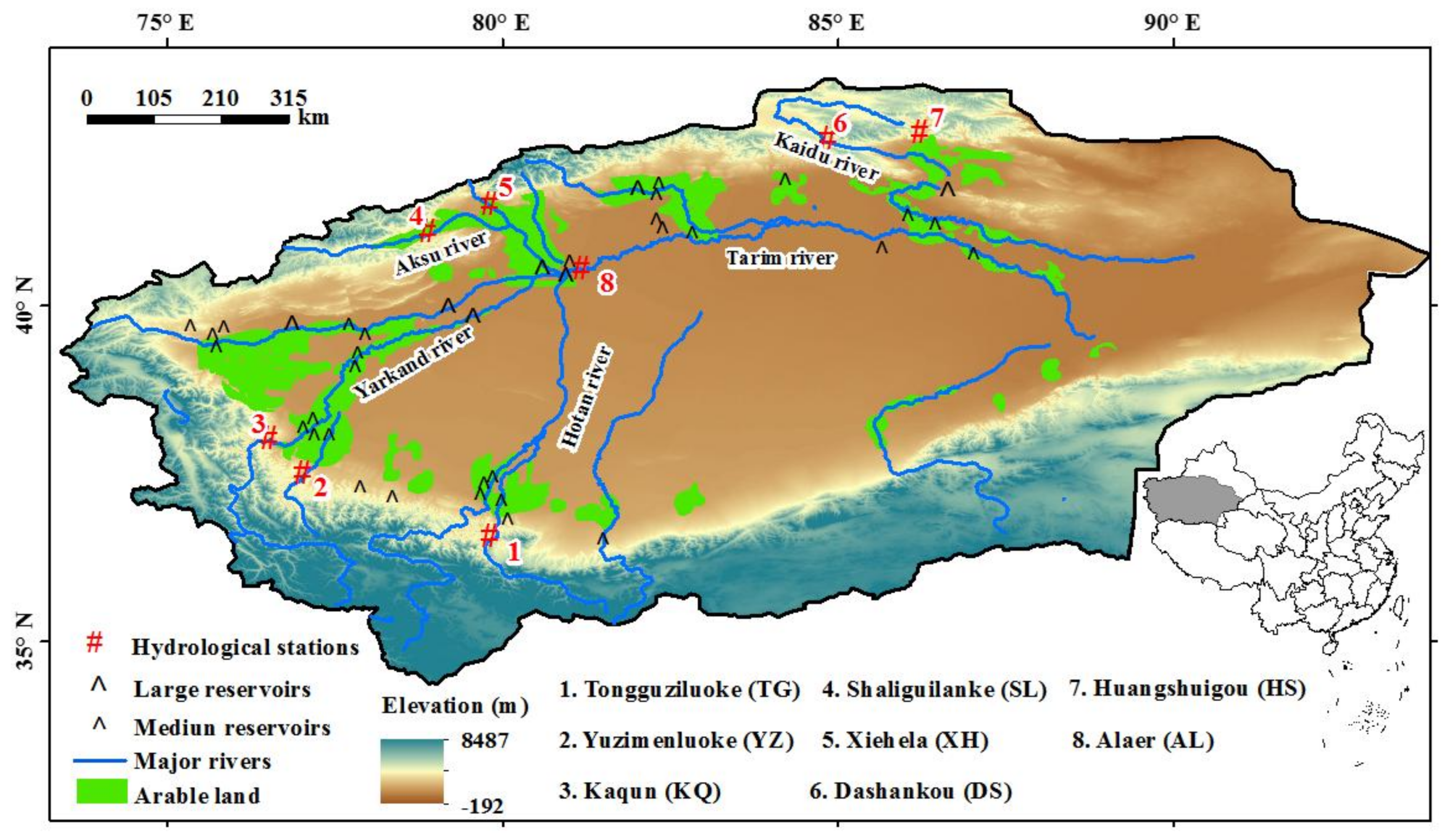
2. Data
3. Methods
3.1. Frequency Analysis
3.2. Copula Function
3.3. Determination of the Generating Function and the Resulting Copula
3.4. Selection of Copula Family
4. Results
4.1. Selection of the Marginal Distributions and Copula Functions
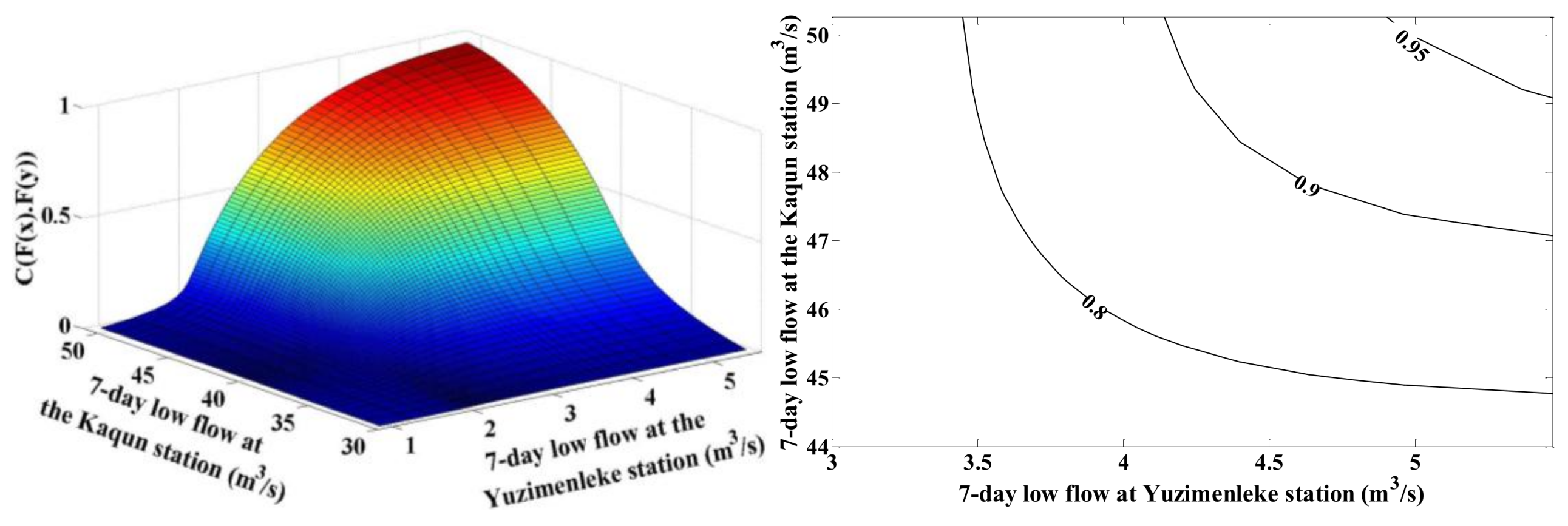
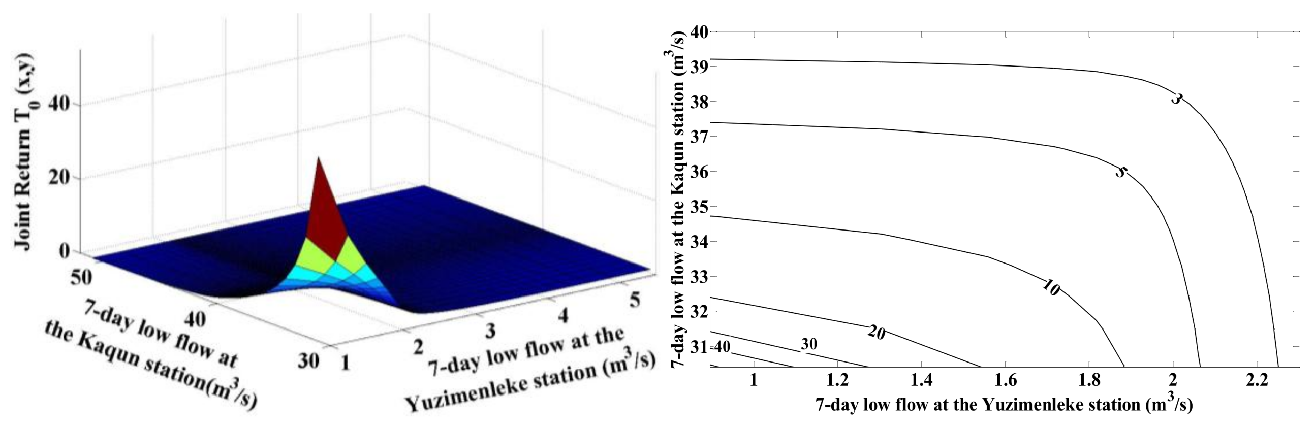
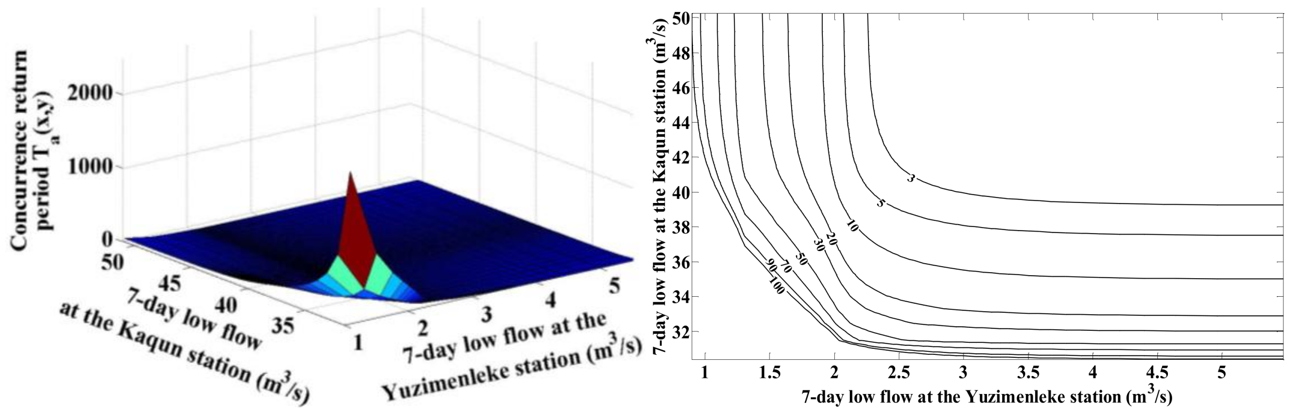
4.2. Joint Probabilistic Behavior of Seven-Day Low Flow Regimes at Different Stations
5. Discussion
6. Conclusions
- (1)
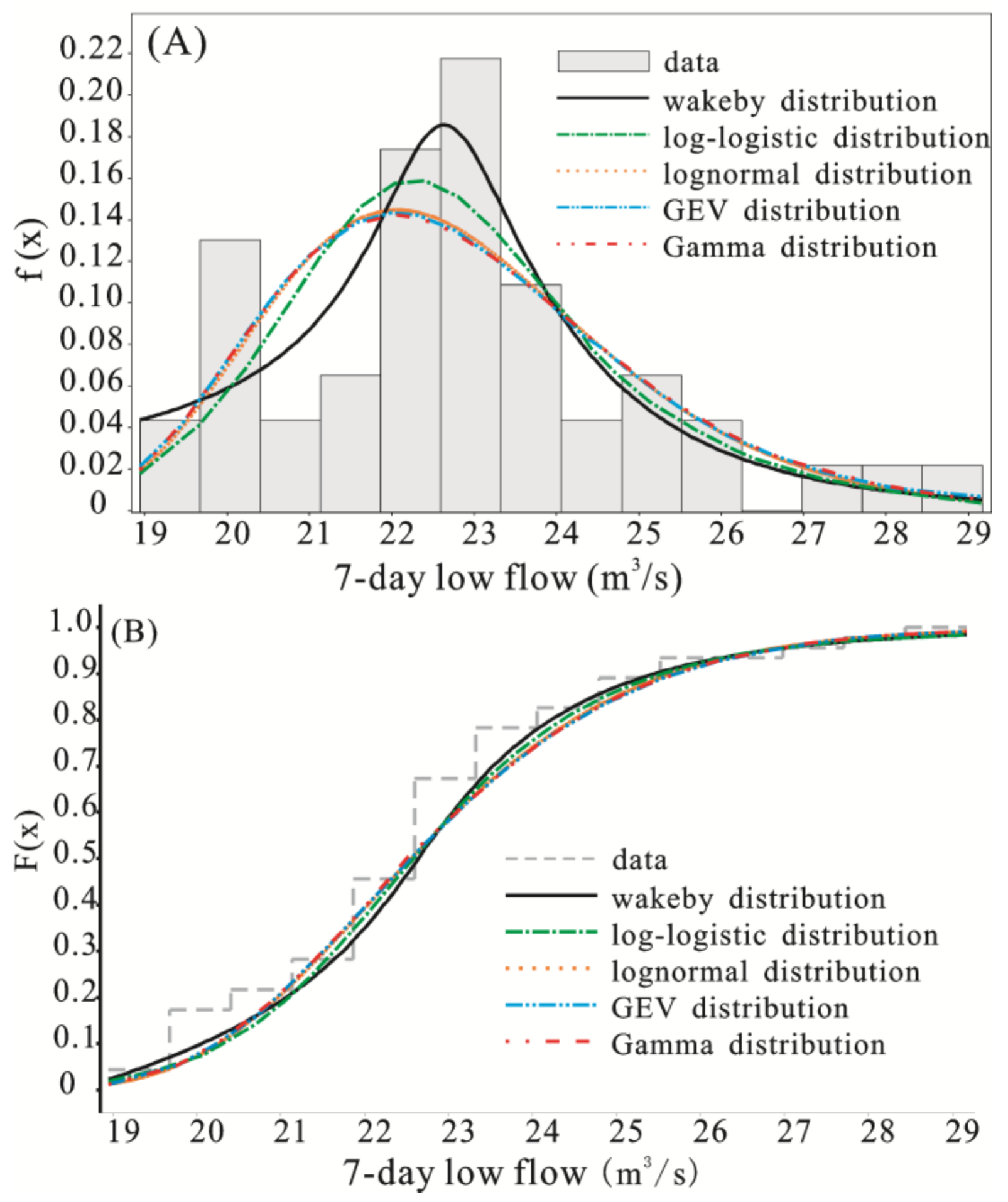
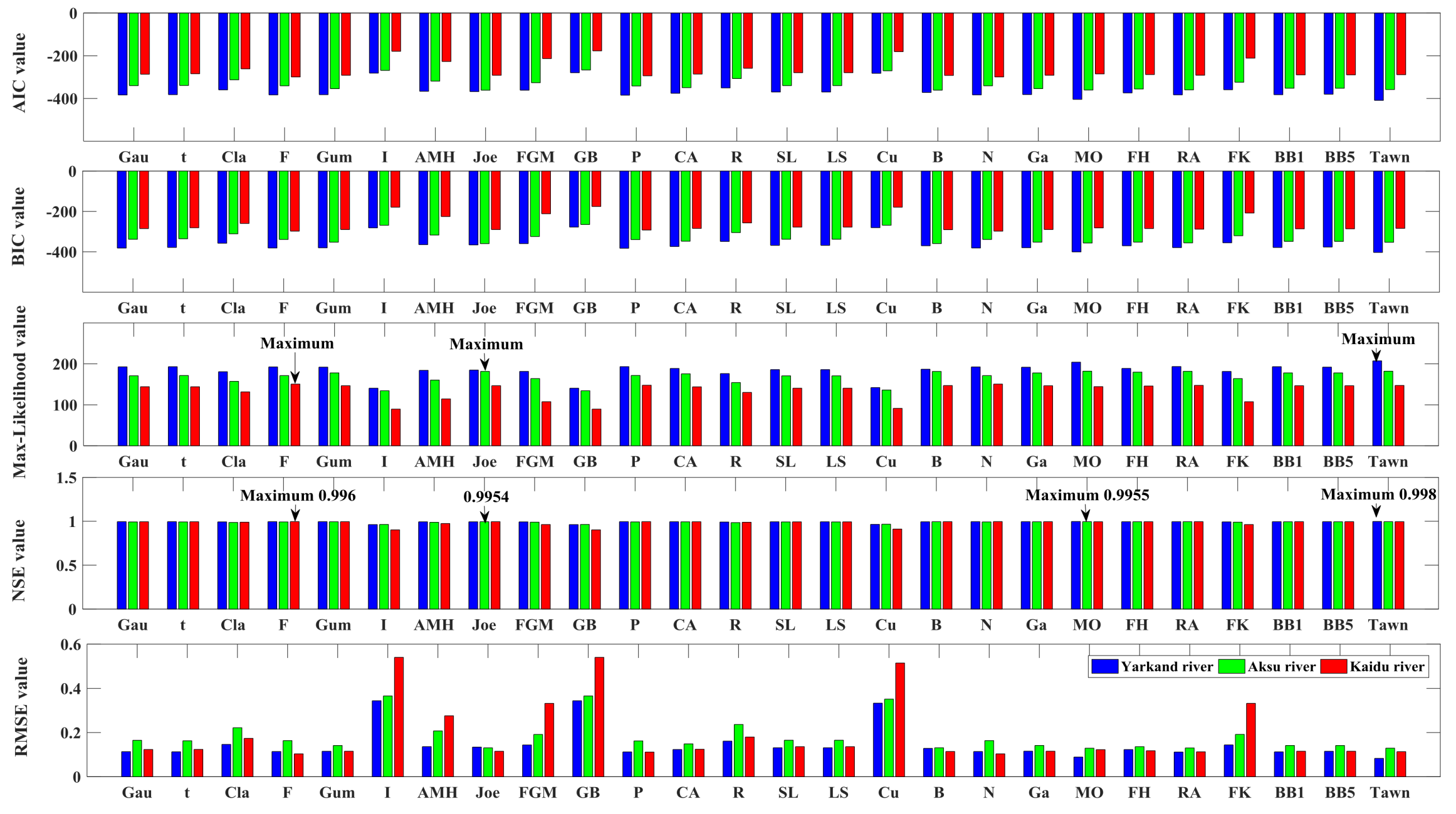
- The Wakeby distribution can be used to describe the probabilistic behavior of the seven-day low flow regimes within the Tarim River Basin. Tawn copula provides a very good fit to the data with a NSE = 0.9978 and is selected as the best copula according to AIC, BIC, maximum likelihood, and other residual-based metrics in Yarkand River Basin. Farlie–Gumbel–Morgenstern copula and Frank copula is the best copula and should be used for further analysis in Aksu River Basin and Kaidu River Basin.
- (2)
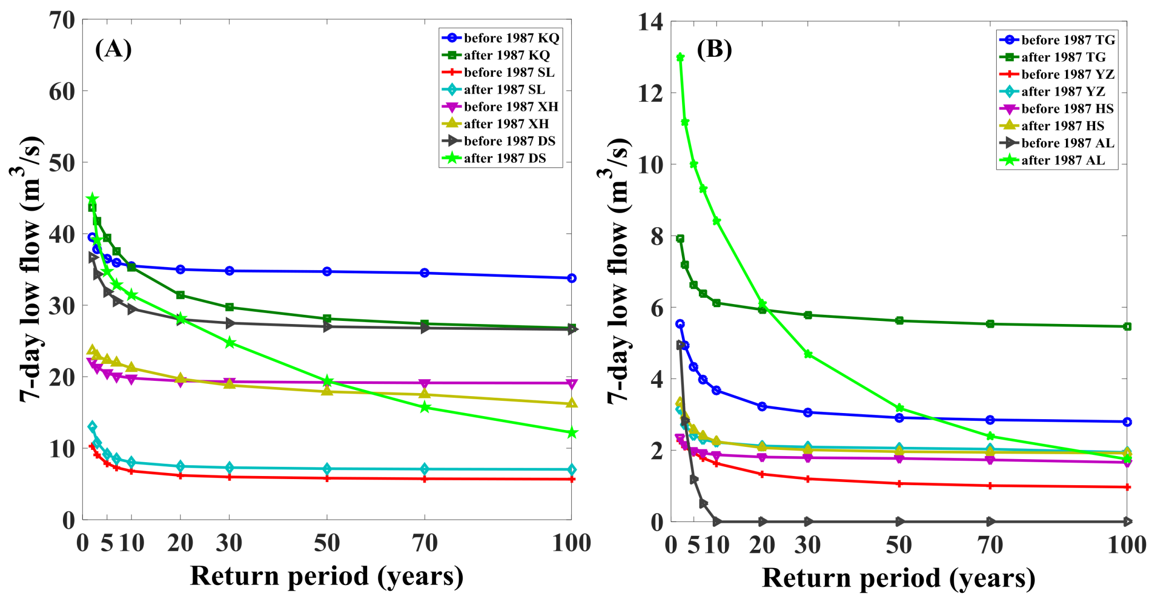
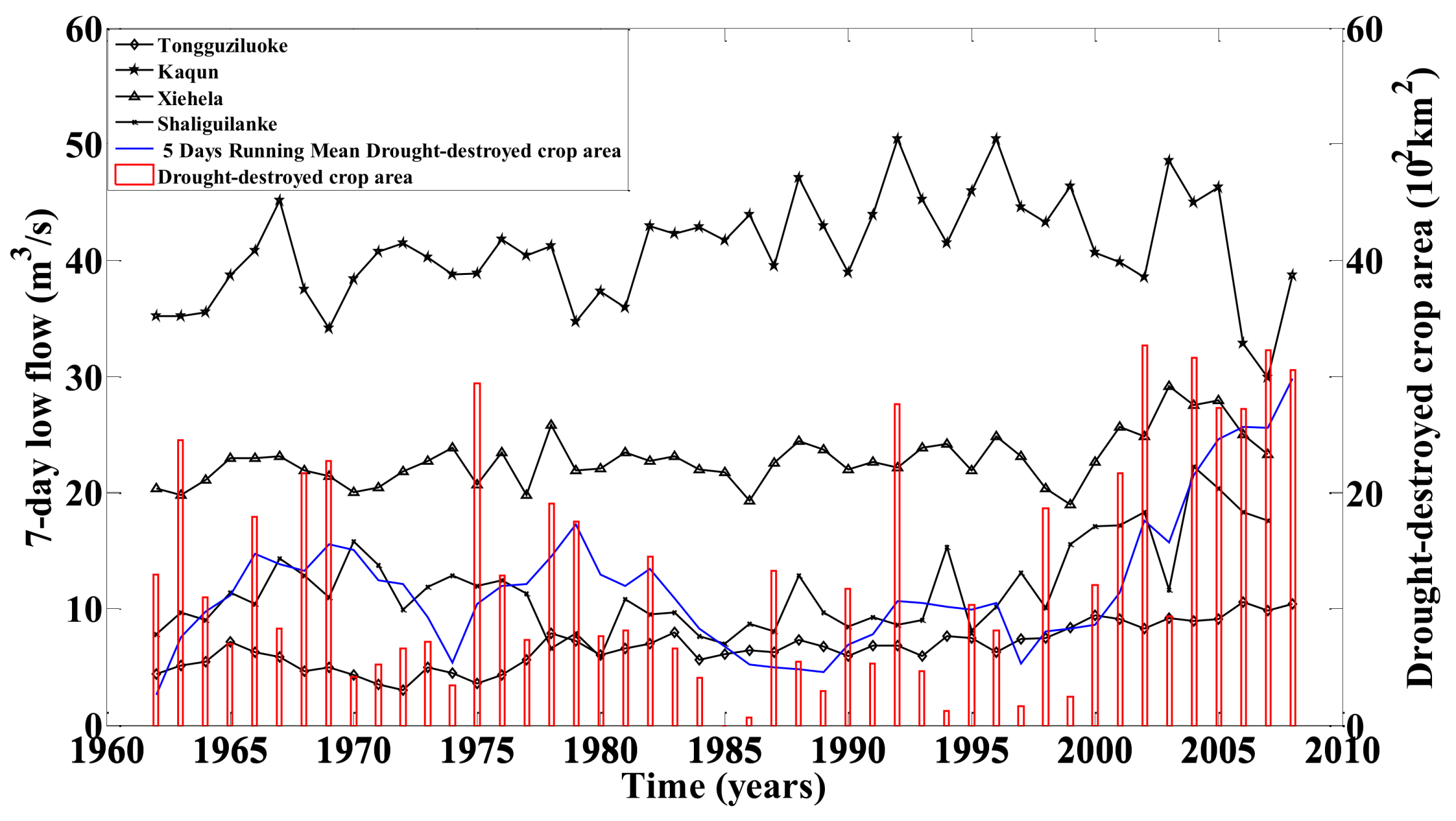
- After 1987, the increase of temperature and precipitation enable the low flow volume to increase to a certain degree. However, the climate change within the Tarim River Basin is uneven in both space and time. Water supply sources in different tributary basins of the Tarim River are different. Hence, the increasing magnitude of the low flow regime is different in different tributaries. However, the massive increase of water demand due to increased irrigated agriculture and livestock farming greatly reduces the streamflow input into the main stem of the Tarim River Basin. Thus, water shortage in the lower Tarim River will not be alleviated.
- (3)
- Hydrological droughts of longer return periods are prone to increasing occurrence frequency. The water supply cannot satisfy the increasing water demand due to significantly increased irrigated arable land and growing population, although the precipitation is increasing and the snowmelt is also increasing due to increased temperature in recent years. The water shortage in Xinjiang is still a challenge for the sustainable development of the local socio-economy. In this case, the development of water-saving technology for irrigated agriculture and effective water resources management is necessary for the sustainable development of regional social economy and conservation of the eco-environment.
Acknowledgments
Author Contributions
Conflicts of Interest
References
- Mirza, M.M.Q. Global warming and changes in the probability of occurrence of floods in Bangladesh and implications. Glob. Environ. Chang. 2002, 12, 127–138. [Google Scholar] [CrossRef]
- Shi, Y.F.; Zhang, Q.; Chen, Z.; Jiang, T.; Wu, J. Channel morphology and its impact on flood passage, the Tianjiazhen reach of the middle Yangtze River. Geomorphology 2007, 85, 176–184. [Google Scholar] [CrossRef]
- Zhang, Q.; Chen, J.; Becker, S. Flood/drought change of last millennium in the Yangtze Delta and its possible connections with Tibetan climatic changes. Glob. Planet. Chang. 2007, 57, 213–221. [Google Scholar] [CrossRef]
- Yan, D.; Xu, T.; Girma, A.; Yuan, Z.; Weng, B.; Qin, T.; Do, P.; Yuan, Y. Regional correlation between precipitation and vegetation in the Huang-Huai-Hai River Basin, China. Water 2017, 9, 557. [Google Scholar] [CrossRef]
- Smakhtin, V.U. Low flow hydrology: A review. J. Hydrol. 2001, 240, 147–186. [Google Scholar] [CrossRef]
- Gao, S.; Liu, P.; Pan, Z.; Ming, B.; Guo, S.; Xiong, L. Derivation of low flow frequency distributions under human activities and its implications. J. Hydrol. 2017, 2017, 549. [Google Scholar] [CrossRef]
- Mishra, A.K.; Singh, P.V. A review of drought concepts. J. Hydrol. 2010, 391, 202–216. [Google Scholar] [CrossRef]
- Foulon, E.; Rousseau, A.N.; Gagnon, P. Development of a methodology to assess future trends in low flows at the watershed scale using solely climate data. J. Hydrol. 2018, 557, 774–790. [Google Scholar] [CrossRef]
- Gumbel, E.J. Statistical forecast of droughts. Bull. Int. Assoc. Sci. Hydrol. 1963, 8, 5–23. [Google Scholar] [CrossRef]
- Palmer, W.C. Meteorologic Drought; Research Paper; US Department of Commerce, Weather Bureau: Washington, DC, USA, 1965; Volume 45, p. 58. [Google Scholar]
- Yu, Y.; Disse, M.; Yu, R.; Yu, G.; Sun, L.; Huttner, P.; Rumbaur, C. Large-scale hydrological modeling and decision-making for agricultural water consumption and allocation in the main stem Tarim River, China. Water 2015, 7, 2821–2839. [Google Scholar] [CrossRef]
- Vörösmarty, C.J.; McIntyre, P.B.; Gessner, M.O.; Dudgeon, D.; Prusevich, A.; Green, P.; Glidden, S.; Bunn, S.E.; Sullivan, C.A.; Reidy Liermann, C.R.; et al. Global threats to human water security and river biodiversity. Nature 2010, 467, 555–561. [Google Scholar] [CrossRef] [PubMed]
- Zhang, J.; Bai, M.; Zhou, S.; Zhao, M. Agricultural water use sustainability assessment in the Tarim River Basin under climatic risks. Water 2018, 10, 170. [Google Scholar] [CrossRef]
- CHEN, Y.N.; Li, W.H.; Xu, C.C.; Hao, X.M. Effects of climate change on water resources in Tarim River Basin, Northwest China. J. Environ. Sci. 2007, 19, 488–493. [Google Scholar] [CrossRef]
- Tao, H.; Gemmer, M.; Bai, Y.; Su, B.; Mao, W. Trends of streamflow in the Tarim River Basin during the past 50 years: Human impact or climate change? J. Hydrol. 2011, 400, 1–9. [Google Scholar] [CrossRef]
- Xu, H.; Ye, M.; Li, J. The water transfer effects on agricultural development in the lower Tarim River, Xinjiang of China. Agric. Water Manag. 2008, 95, 59–68. [Google Scholar] [CrossRef]
- Zhang, Q.; Chen, Y.D.; Chen, X.; Li, J. Copula-based analysis of hydrological extremes and implications of hydrological behaviors in the Pearl River basin, China. J. Hydrol. Eng. 2011, 16, 598–607. [Google Scholar] [CrossRef]
- Zhang, Q.; Li, J.F.; Chen, Y.Q.; Chen, X.H. Observed changes of temperature extremes during 1960–2005 in China: Natural or human-induced variations? Theor. Appl. Climatol. 2011, 106, 417–431. [Google Scholar] [CrossRef]
- Gu, X.; Zhang, Q.; Singh, V.P.; Chen, Y.D.; Shi, P. Temporal clustering of floods and impacts of climate indices in the Tarim River Basin, China. Glob. Planet. Chang. 2016, 147, 12–24. [Google Scholar] [CrossRef]
- Gu, X.; Zhang, Q.; Singh, V.P.; Chen, X.; Liu, L. Nonstationarity in the occurrence rate of floods in the Tarim River Basin, China, and related impacts of climate indices. Glob. Planet. Chang. 2016, 142, 1–13. [Google Scholar] [CrossRef]
- Li, Z.; Hao, Z.; Shi, X.; Déry, S.J.; Li, J.; Chen, S.; Li, Y. An agricultural drought index to incorporate the irrigation process and reservoir operations: A case study in the Tarim River Basin. Glob. Planet. Chang. 2016, 143, 10–20. [Google Scholar] [CrossRef]
- Xu, Z.; Liu, Z.; Fu, G.; Chen, Y. Trends of major hydroclimatic variables in the Tarim River Basin during the past 50 years. J. Arid Environ. 2010, 74, 256–267. [Google Scholar] [CrossRef]
- Maidment, R.D. Handbook of Hydrology; McGraw-Hill Professional: New York, NY, USA, 1993. [Google Scholar]
- Svensson, C.; Kundzewicz, Z.W.; Maurer, T. Trend detection in river flow series: 2. Flood and low-flow index series. Hydrol. Sci. J. 2005, 50, 811–824. [Google Scholar] [CrossRef]
- Park, J.S.; Jung, H.S.; Kim, R.S.; Oh, J.H. Modeling summer extreme rainfall over the Korean Peninsula using Wakeby distribution. Int. J. Climatol. 2001, 21, 1371–1384. [Google Scholar] [CrossRef]
- Mares, C.; Mares, H.; Stanciu, A. Extreme value analysis in the Danube lower basin discharge time series in the twentieth century. Theor. Appl. Climatol. 2009, 95, 223–233. [Google Scholar] [CrossRef]
- Hosking, J.R.M. L-moments: Analysis and estimation of distributions using linear combinations of order statistics. J. Roy. Stat. Soc. Ser. B 1990, 52, 105–124. [Google Scholar]
- De Michele, C.; Salvadori, G.; Canossi, M.; Petaccia, A.; Rosso, R. Bivariate statistical approach to check adequacy of dam spillway. J. Hydrol. Eng. 2005, 10, 50–57. [Google Scholar] [CrossRef]
- Zhang, L.; Singh, V.P. Bivariate flood frequency analysis using the copula method. J. Hydrol. Eng. 2006, 11, 150–164. [Google Scholar] [CrossRef]
- Zhang, L.; Singh, V.P. Bivariate rainfall frequency distributions using Archimedean copulas. J. Hydrol. 2007, 332, 93–109. [Google Scholar] [CrossRef]
- Zhang, L.; Singh, V.P. Gumbel–Hougaard copula for trivariate rainfall frequency analysis. J. Hydrol. Eng. 2007, 12, 409–419. [Google Scholar] [CrossRef]
- Kao, S.C.; Govindaraju, R.S. A copula-based joint deficit index for droughts. J. Hydrol. 2010, 380, 121–134. [Google Scholar] [CrossRef]
- Genest, C.; Mackay, L. The joy of copulas: Bivariate distributions with uniform marginals. Am. Stat. 1986, 40, 280–283. [Google Scholar]
- Sadegh, M.; Ragno, E.; Aghakouchak, A. Multivariate Copula Analysis Toolbox (MvCAT): Describing dependence and underlying uncertainty using a Bayesian framework. Water Res. Res. 2017, 53, 5166–5183. [Google Scholar] [CrossRef]
- Genest, C.; Favre, A.C. Everything you always wanted to know about copula modeling but were afraid to ask. J. Hydrol. Eng. 2007, 12, 347–368. [Google Scholar] [CrossRef]
- Poulin, A.; Huard, D.; Favre, A.C.; Pugin, S. Importance of tail dependence in bivariate frequency analysis. J. Hydrol. Eng. 2007, 12, 394–403. [Google Scholar] [CrossRef]
- Praprom, C.; Sriboonchitta, S. Extreme Value Copula Analysis of Dependences between Exchange Rates and Exports of Thailand. Adv. Intell. Syst. Comput. 2014, 251, 187–199. [Google Scholar]
- Li, C.; Singh, V.P.; Mishra, A.K. A bivariate mixed distribution with a heavy-tailed component and its application to single-site daily rainfall simulation. Water Res. Res. 2013, 49, 767–789. [Google Scholar] [CrossRef]
- Clayton, D.G. A model for association in bivariate life tables and its application in epidemiological studies of familial tendency in chronic disease incidence. Biometrika 1978, 65, 141–151. [Google Scholar] [CrossRef]
- Nelsen, R.B. An Introduction to Copulas; Springer: New York, NY, USA, 2007. [Google Scholar]
- Ali, M.M.; Mikhail, N.; Haq, M.S. A class of bivariate distributions including the bivariate logistic. J. Multivar. Anal. 1978, 8, 405–412. [Google Scholar] [CrossRef]
- Gumbel, E.J. Bivariate exponential distributions. J. Am. Stat. Assoc. 1960, 55, 698–707. [Google Scholar] [CrossRef]
- Barnett, V. Some bivariate uniform distributions. Commun. Stat. Theory Methods 1980, 9, 453–461. [Google Scholar] [CrossRef]
- Plackett, R.L. A class of bivariate distributions. J. Am. Stat. Assoc. 1965, 60, 516–522. [Google Scholar] [CrossRef]
- Cuadras, C.M.; Auge, J. A continuous general multivariate distribution and its properties. Commun. Stat. Theory Methods 1981, 10, 339–353. [Google Scholar] [CrossRef]
- Shih, J.H.; Louis, T.A. Inferences on the association parameter in copula models for bivariate survival data. Biometrics 1995, 51, 1384–1399. [Google Scholar] [CrossRef] [PubMed]
- Joe, H. Dependence Modeling with Copulas; CRC Press: Boca Raton, FL, USA, 2014. [Google Scholar]
- Durrleman, V.; Nikeghbali, A.; Roncalli, T. A note about the conjecture on Spearman’s rho and Kendall’s tau. Soc. Sci. Electron. Pub. 2007. [Google Scholar] [CrossRef]
- Frees, E.W.; Valdez, E.A. Understanding relationships using copulas. N Am. Actuar. J. 1998, 2, 1–25. [Google Scholar] [CrossRef]
- Huynh, V.N.; Kreinovich, V.; Sriboonchitta, S. Modeling Dependence in Econometrics; Springer: New York, NY, USA, 2014. [Google Scholar]
- Fischer, M.; Hinzmann, G. A New Class of Copulas with Tail Dependence and a Generalized Tail Dependence Estimator; Citeseer, Friedrich-Alexander University Erlangen-Nuremberg: Erlangen, Germany, 2007. [Google Scholar]
- Roch, O.; Alegre, A. Testing the bivariate distribution of daily equity returns using copulas. An application to the Spanish stock market. Comput. Stat. Data Anal. 2006, 51, 1312–1329. [Google Scholar] [CrossRef]
- Genest, C.; Rivest, L. Statistical inference procedures for bivariate Archimedean copulas. J. Am. Stat. Assoc. 1993, 88, 1034–1043. [Google Scholar] [CrossRef]
- Geweke, J. Exact predictive densities for linear models with arch disturbances. J. Econom. 1989, 40, 63–86. [Google Scholar] [CrossRef]
- Geweke, J. Bayesian inference in econometric models using Monte Carlo integration. Econometrica 1989, 57, 1317–1339. [Google Scholar] [CrossRef]
- Cheng, L.; AghaKouchak, A.; Gilleland, E.; Katz, R.W. Non-stationary extreme value analysis in a changing climate. Clim. Chang. 2014, 127, 353–369. [Google Scholar] [CrossRef]
- Andrieu, C.; Thoms, J. A tutorial on adaptive MCMC. Stat. Comput. 2008, 18, 343–373. [Google Scholar] [CrossRef]
- Akaike, H. A new look at the statistical model identification. IEEE Trans. Autom. Control 1974, 19, 716–723. [Google Scholar] [CrossRef]
- Akaike, H. Information theory and an extension of the maximum likelihood principle. Int. Symp. Inf. Theory 2014, 1, 610–624. [Google Scholar]
- Aho, K.; Derryberry, D.; Peterson, T. Model selection for ecologists: The worldviews of AIC and BIC. Ecology 2014, 95, 631–636. [Google Scholar] [CrossRef] [PubMed]
- Schwarz, G. Estimating the dimension of a model. Ann. Math. Stat. 1978, 6, 461–464. [Google Scholar] [CrossRef]
- Öztekin, T. Wakeby distribution for representing annual extreme and partial duration rainfall series. Meteorological Applications 2007, 14, 381–387. [Google Scholar] [CrossRef]
- Griffiths, G.A. A theoretically based Wakeby distribution for annual flood series. Hydrol. Sci. J. 1989, 34, 231–248. [Google Scholar] [CrossRef]
- Shi, Y.F.; Shen, Y.P.; Li, D.L.; Zhang, G.W.; Ding, Y.J.; Hu, R.J.; Kang, E.S. Discussion on the present climate change from warm-dry to warm-wet in Northwest China. Quat. Sci. 2003, 23, 152–164. [Google Scholar]
- Zhang, Q.; Singh, V.P.; Li, J.; Jiang, F.; Bai, Y. Spatio-temporal variations of precipitation extremes in Xinjiang, China. J. Hydrol. 2012, 434–435, 7–18. [Google Scholar] [CrossRef]
- Mansur, S.; Nurkamil, Y. Oasis land use change and its hydrological response to Tarim River Basin. Geogr. Res. 2010, 29, 2251–2260. [Google Scholar]
- Zhang, Q.; Xu, C.-Y.; Tao, H.; Jiang, T.; Chen, Y.D. Climate changes and their impacts on water resources in the arid regions: A case study of the Tarim River basin, China. Stoch. Environ. Res. Risk Assess. 2010, 24, 349–358. [Google Scholar] [CrossRef]
- Sun, B.G.; Mao, W.Y.; Feng, Y.R.; Chang, T.; Zhang, L.P.; Zhao, L. Study on the change of air temperature, precipitation and runoff volume in the Yarkand River basin. Arid Zone Res. 2006, 23, 203–209. [Google Scholar]
- Ding, M.J. Theories and Practices of Water Resources Management of the Tarim River Basin China; Science Press: Beijing, China, 2009. [Google Scholar]
- Sun, X.J.; Zhao, C.Y.; Zheng, J.F. Climate changes of the Aksu River basin in recent 46 years. J. Arid Land Res. Environ. 2011, 25, 78–83. [Google Scholar]
- Zhang, Y.; Li, B.; Cheng, W.; Zhang, X. Response of streamflow changes of the Kaidu River to climate changes. Res. Sci. 2004, 26, 69–76. [Google Scholar]
- Sun, P.; Zhang, Q.; Lu, X.; Bai, Y. Changing properties of low flow of the Tarim River basin: Possible causes and implications. Quat. Int. 2012, 282, 78–86. [Google Scholar] [CrossRef]


| No. | Stations | Abbreviation | Streamflow Series | Basin |
|---|---|---|---|---|
| 1 | Tongguziluoke | TG | 1962–13 December 2008 | Hotan river |
| 2 | Yuzimenluoke | YZ | 1 January 1962–13 December 2008 | Yarkand river |
| 3 | Kaqun | KQ | 1 January 1962–13 December 2008 | Yarkand river |
| 4 | Shaliguilanke | SL | 1 January 1962–13 December 2008 | Aksu river |
| 5 | Xiehela | XH | 1 January 1962–13 December 2008 | Aksu river |
| 6 | Dashankou | DS | 1 January 1972–13 December 2008 | Kaidu river |
| 7 | Huangshuigou | HS | 1 January 1972–13 December 2008 | Kaidu river |
| 8 | Alaer | AL | 1 January 1962–13 December 2008 | Mainstrean of Tarim river |
| Name | Abbreviation | Mathematical Descriptiona | Parameter Range | Reference |
|---|---|---|---|---|
| Gaussian | Gau | [38] | ||
| t | t | [38] | ||
| Clayton | Cla | [39] | ||
| Frank | F | [38] | ||
| Gumbel | Gum | [38] | ||
| Independence | I | [40] | ||
| Ali–Mikhail–Haq | AMH | [41] | ||
| Joe | Joe | [38] | ||
| Farlie–Gumbel–Morgenstern | FGM | [40] | ||
| Gumbel–Barnett | GB | [42,43] | ||
| Plackett | P | [44] | ||
| Cuadras-Auge | CA | [45] | ||
| Raftery | R | [40] | ||
| Shih-Louis | SL | [46] | ||
| Linear-Spearman | LS | [47] | ||
| Cubic | Cu | [48] | ||
| Burr | B | [49] | ||
| Nelsen | N | [40] | ||
| Galambos | Ga | [50] | ||
| Marshall–Olkin | MO | [50] | ||
| Fischer–Hinzmann | FH | [51] | ||
| Roch–Alegre | RA | [52] | ||
| Fischer–Kock | FK | [34] | ||
| BB1 | BB1 | [35] | ||
| BB5 | BB5 | [35] | ||
| Tawn | Tawn | [50] |
| Hydrological Stations | TG | YZ | KQ | SL | XH | DS | HS | AL | |
|---|---|---|---|---|---|---|---|---|---|
| Probability Functions | |||||||||
| Wakeby (5P) | 0.043 | 0.058 | 0.059 | 0.046 | 0.057 | 0.089 | 0.060 | 0.071 | |
| Weibull (3P) | 0.042 | 0.096 | 0.055 | 0.063 | 0.094 | 0.144 | 0.076 | 0.162 | |
| Gamma (3P) | 0.041 | 0.083 | 0.054 | 0.058 | 0.085 | 0.130 | 0.070 | 0.128 | |
| Lognormal (3P) | 0.041 | 0.075 | 0.049 | 0.057 | 0.081 | 0.106 | 0.075 | 0.182 | |
| Log-logistic (3P) | 0.046 | 0.067 | 0.055 | 0.054 | 0.070 | 0.102 | 0.075 | 0.193 | |
| General Pareto (3P) | 0.081 | 0.088 | 0.097 | 0.056 | 0.119 | 0.119 | 0.064 | 0.111 | |
| Gen. Extreme Value (3P) | 0.045 | 0.062 | 0.055 | 0.057 | 0.083 | 0.094 | 0.077 | 0.074 | |
| Maximum Extreme Value (3P) | 0.062 | 0.070 | 0.105 | 0.048 | 0.098 | 0.107 | 0.079 | 0.153 | |
| Beta (4P) | 0.072 | 0.084 | 0.052 | 0.063 | 0.086 | 0.132 | 0.081 | 0.401 | |
| Gumbel Max Distribution (2P) | 0.072 | 0.078 | 0.082 | 0.073 | 0.092 | 0.085 | 0.081 | 0.099 | |
| Gumbel Min Distribution (2P) | 0.123 | 0.194 | 0.111 | 0.181 | 0.158 | 0.224 | 0.204 | 0.122 | |
| Stations | α | β | γ | δ | ξ |
|---|---|---|---|---|---|
| TG | 18.90 | 9.08 | 3.02 | −0.41 | 2.63 |
| YZ | 41.28 | 31.35 | 1.02 | −0.05 | 0.53 |
| KQ | 70.26 | 9.52 | 6.20 | −0.35 | 29.67 |
| SL | 935.35 | 131.39 | 5.82 | −0.24 | 0 |
| XH | 16.82 | 5.44 | 1.48 | 0.09 | 18.55 |
| DS | 1836.5 | 61.10 | 14.15 | −0.22 | 0 |
| HS | 47.92 | 58.27 | 1.20 | 10.37 | 1.06 |
| AL | 21.78 | 1.99 | 2.57 | 0.19 | −1.35 |
| Stations | T = 2 | T = 3 | T = 5 | T = 7 | T = 10 | T = 20 | T = 30 | T = 50 | T = 70 | T = 100 |
|---|---|---|---|---|---|---|---|---|---|---|
| TG | 5.53 | 4.94 | 4.33 | 3.98 | 3.67 | 3.23 | 3.06 | 2.91 | 2.85 | 2.80 |
| YZ | 2.26 | 2.09 | 1.92 | 1.78 | 1.63 | 1.33 | 1.20 | 1.07 | 1.01 | 0.97 |
| KQ | 39.5 | 37.8 | 36.5 | 35.9 | 35.5 | 35.0 | 34.8 | 34.7 | 34.5 | 33.8 |
| SL | 10.3 | 9.05 | 7.87 | 7.28 | 6.80 | 6.20 | 5.98 | 5.81 | 5.73 | 5.67 |
| XH | 22.1 | 21.3 | 20.5 | 20.1 | 19.8 | 19.4 | 19.3 | 19.2 | 19.14 | 19.11 |
| DS | 36.7 | 34.3 | 31.9 | 30.6 | 29.5 | 28.0 | 27.5 | 27.0 | 26.8 | 26.6 |
| HS | 2.36 | 2.15 | 1.99 | 1.92 | 1.87 | 1.81 | 1.79 | 1.77 | 1.73 | 1.66 |
| AL | 4.95 | 2.83 | 1.20 | 0.51 | 0 | 0 | 0 | 0 | 0 | 0 |
| Stations | T = 2 | T = 3 | T = 5 | T = 7 | T = 10 | T = 20 | T = 30 | T = 50 | T = 70 | T = 100 |
|---|---|---|---|---|---|---|---|---|---|---|
| TG | 7.93 | 7.18 | 6.62 | 6.38 | 6.12 | 5.93 | 5.78 | 5.62 | 5.53 | 5.46 |
| YZ | 3.14 | 2.71 | 2.42 | 2.30 | 2.22 | 2.12 | 2.09 | 2.06 | 2.03 | 1.94 |
| KQ | 43.6 | 41.8 | 39.4 | 37.5 | 35.3 | 31.4 | 29.7 | 28.1 | 27.4 | 26.8 |
| SL | 13.0 | 10.8 | 9.16 | 8.50 | 8.02 | 7.47 | 7.29 | 7.14 | 7.08 | 7.04 |
| XH | 23.6 | 22.9 | 22.3 | 21.9 | 21.2 | 19.7 | 18.8 | 17.9 | 17.5 | 16.2 |
| DS | 44.9 | 39.1 | 34.7 | 32.8 | 31.4 | 28.1 | 24.8 | 19.4 | 15.7 | 12.2 |
| HS | 3.34 | 2.95 | 2.57 | 2.39 | 2.24 | 2.07 | 2.01 | 1.96 | 1.94 | 1.92 |
| AL | 13.0 | 11.2 | 10.0 | 9.31 | 8.41 | 6.10 | 4.69 | 3.18 | 2.39 | 1.75 |
| Joint Distribution of Seven-Day Low Flow | Copula | θ1 | θ2 | θ3 |
|---|---|---|---|---|
| YZ and KQ stations | Tawn | 0.394 | 0.931 | 3.014 |
| SL and XH stations | Farlie–Gumbel–Morgenstern | 1.874 | - | - |
| DS and HS stations | Frank | 6.715 | - | - |
| Designed Return Periods T | YZ and KQ Stations | SL and XH Station | DS and HS Stations | |||
|---|---|---|---|---|---|---|
| JRP T0 | CRP Ta | JRP T0 | CRP Ta | JRP T0 | CRP Ta | |
| 2 | 1.5 | 3.1 | 1.6 | 2.7 | 1.4 | 3.6 |
| 5 | 3.1 | 13.7 | 3.4 | 9.6 | 2.9 | 19.9 |
| 10 | 5.7 | 42.5 | 6.2 | 25.5 | 5.4 | 74.7 |
| 20 | 10.8 | 131.4 | 11.7 | 67.6 | 10.4 | 288.8 |
| 30 | 15.9 | 254.3 | 17.2 | 119.5 | 15.4 | 641.9 |
| 50 | 26.1 | 584.3 | 27.8 | 245.1 | 25.4 | 1765.3 |
| 70 | 36.3 | 1010.6 | 38.4 | 393.4 | 35.4 | 3445.1 |
| 90 | 46.4 | 1521.6 | 48.9 | 560.2 | 45.4 | 5681.2 |
| 100 | 51.4 | 1806.4 | 54.2 | 649.6 | 50.4 | 7007.9 |
| River | Number of Water Reservoirs | Total Storage Capacity/108m3 | Utilizable Capacity/108m3 | Cumulative Irrigated Areas/hm2 | Effective Irrigated Areas/hm2 | Designed Flood Volum/108m3 |
|---|---|---|---|---|---|---|
| Hetian River Basin | 20 | 2.35 | 2.05 | 36,263.04 | 33,268.3 | 2.20 |
| Yarkand River Basin | 37 | 14.20 | 11.57 | 303,816.3 | 201,283.4 | 19.97 |
| Aksu River Basin | 6 | 4.90 | 4.20 | 105,116.2 | 80,870.7 | 4.14 |
| Kaidu River Basin | 5 | 0.77 | 0.52 | - | - | 0.48 |
| Mainstem of the Tarim River Basin | 8 | 5.86 | 4.76 | 66,326.7 | 49,969.2 | 9.20 |
| Total | 76 | 28.08 | 23.10 | 511,522.2 | 365,391.6 | 35.99 |
| River | Number of Water Supply Facilities | Designed Irrigated Areas/hm2 | Effective Irrigated Areas/hm2 | Designed Water Supply Capacity/m3/s | Standing Water Supply Capacity/m3/s | Standing Water Supply Rate/% |
|---|---|---|---|---|---|---|
| Hetian River Basin | 27 | 62,903.15 | 48,402.42 | 81.40 | 62.60 | 76.90 |
| Yarkand River Basin | 26 | 1,155,391 | 329,349.8 | 220.30 | 169.50 | 76.94 |
| Aksu River Basin | 63 | 702,035.1 | 570,028.5 | 198.60 | 165.50 | 83.33 |
| Kaidu-Kongque River Basin | 32 | 244,945.6 | 201,343.4 | 89.12 | 74.26 | 83.33 |
| Mainstem of the Tarim River Basin | 138 a | 85,370.94 | 79,937.33 | 293.00 | 293.00 | 100.00 |
| Total | 286 | 2,250,646 | 1,229,061 | 882.42 | 764.86 | 86.68 |
© 2018 by the authors. Licensee MDPI, Basel, Switzerland. This article is an open access article distributed under the terms and conditions of the Creative Commons Attribution (CC BY) license (http://creativecommons.org/licenses/by/4.0/).
Share and Cite
Sun, P.; Zhang, Q.; Yao, R.; Singh, V.P.; Song, C. Low Flow Regimes of the Tarim River Basin, China: Probabilistic Behavior, Causes and Implications. Water 2018, 10, 470. https://doi.org/10.3390/w10040470
Sun P, Zhang Q, Yao R, Singh VP, Song C. Low Flow Regimes of the Tarim River Basin, China: Probabilistic Behavior, Causes and Implications. Water. 2018; 10(4):470. https://doi.org/10.3390/w10040470
Chicago/Turabian StyleSun, Peng, Qiang Zhang, Rui Yao, Vijay P. Singh, and Changqing Song. 2018. "Low Flow Regimes of the Tarim River Basin, China: Probabilistic Behavior, Causes and Implications" Water 10, no. 4: 470. https://doi.org/10.3390/w10040470