Discharge Coefficient of Rectangular Short-Crested Weir with Varying Slope Coefficients

Abstract

Rectangular short-crested weirs are widely used for simple structure and high discharge capacity. As one of the most important and influential factors of discharge capacity, side slope can improve the hydraulic characteristics of weirs at special conditions. In order to systemically study the effects of upstream and downstream slope coefficients S₁ and S₂ on overflow discharge coefficient in a rectangular short-crested weir the Volume of Fluid (VOF) method and the Renormalization Group (RNG) κ-ε turbulence model are used. In this study, the slope coefficient ranges from V to 3H:1V and each model corresponds to five total energy heads of H₀ ranging from 8.0 to 24.0 cm. Comparisons of discharge coefficients and free surface profiles between simulated and laboratory results display a good agreement. The simulated results show that the difference of discharge coefficients will decrease with upstream slopes and increase with downstream slopes as H₀ increases. For a given H₀, the discharge coefficient has a convex parabolic relation with S₁ and a piecewise linearity relation with S₂. The maximum discharge coefficient is always obtained at S₂ = 0.8. There exists a difference between upstream and downstream slope coefficients in the influence range of free surface curvatures. Furthermore, a proposed discharge coefficient equation by nonlinear regression is a function of upstream and downstream slope coefficients.

1. Introduction

As common hydraulic engineering structures, low weirs are widely used to measure discharge in irrigation systems and to increase upstream water level in hydroelectric projects. Flat-topped weirs of finite crest length are classified into four types: long-crested weir (0 < H/δ ≤ 0.1), broad-crested weir (0.1 ≤ H/δ ≤ 0.4), short-crested weir (0.4 ≤ H/δ ≤ 1.5–1.9), and sharp-crested weir (1.5–1.9 ≤ H/δ), depending on the relative length of crest H/δ, where H is the crest depth over weir at free overflow condition and δ is the length of weir crest in the streamwise direction [1]. The flat-topped low weirs generally include broad-crested weir and short-crested weir. Under the same inflow condition, the discharge coefficient of short-crested weir is approximately 0.33–0.46, while that of broad-crested weir is 0.32–0.385, hence the former is stronger than the latter in terms of discharge capacity. The short-crested weirs are designed into curvilinear profile and broken-line profile according to the longitudinal profile. The former is usually used as a high weir and the latter as a low weir. Considering as the small overflow weirs, although the discharge coefficient of former is larger, the latter is widely used in view of the convenience of construction. The broken-line short-crested weir is classified into rectangular profile and trapezoidal profile according to the longitudinal profile [2]. Moreover, the rectangular short-crested weir is insensitive to the downstream submergence, and in special situations the geometrical configuration could be flexibly modified so as to increase discharge capacity and avoid cavitation damage of weir flow structures [3].

Extensive experimental and numerical studies on weir height and weir crest length of the short-crested weir were carried out [4,5,6,7], and the corresponding discharge coefficient formulae have been derived [1,8,9,10]. Although the existing research displays a close relation between slope coefficient and discharge coefficient of broad-crested weirs [10,11,12], recently there has been little research on the effect of slope coefficient on short-crested weirs[4,6]. Azimi et al. [13] found that flow separated from the entrance of crest, and this part of flow would reattach to the weir crest with curvilinear flow existing over the entire weir before it left the crest again. Goodarzi et al. [14] showed that the size of flow separation space at the entrance of weir crest varied with upstream slope, which indirectly resulted in variation of discharge coefficients. Bos [4] found that a higher streamline curvature above the weir crest and a smaller size on separation region had a positive influence on the head-discharge relationship of weirs. Farhoudi et al. [15] concluded that decreasing upstream slope angle increased the discharge coefficient until it reached the maximum value at α = 25° (2.1H:1V). Compared with a rectangular weir with a sloped upstream weir face, Sargison et al. [16] found that the weir with sloped downstream weir face could improve the discharge capacity. Recently, Tong et al. [10,17] have carried out much work on investigating the flow characteristics of short-crested weir and concluded that the maximum discharge coefficient existed at S₁ = 2.0–3.0. Chen et al. [18,19] analyzed the effect of upstream slope on the discharge coefficient by combining experiments and numerical simulations. Li et al. [20] pointed that the discharge coefficient of rectangular short-crested weir with S₁ = 0.5 is 2.0% larger than that of the rectangular short-crested weir, and the flow regime of the former was better than the latter. Haun et al. [21] applied computational fluid dynamics (CFD) software Flow-3D [22] to simulate the free overflow over the trapezoidal broad-crested weir, and the results were in good agreement with the experimental data [16]. Paik et al. [23] used the RNG κ-ε turbulent model to calculate the two flow separation zones for free overflow over the rectangular broad-crested weir, which fit well with those of physical models. In conclusion, the approach of numerical simulation meets the requirement of studying the hydraulic characteristics of the free surface weir flow.

Almost all of the above conclusions are premised on the inflow discharge, whereas this study is premised on the total energy head H₀ over the crest to realize the flexible manipulation in engineering. Besides, the previous research on the discharge coefficient has not taken the slope coefficients into consideration [1,10]. In order to meet the demand of high accuracy on applicability and construction design, performing research on the effect of slope coefficients on discharge capacity is necessary. The present paper uses the Flow-3D software to simulate the free overflow over the rectangular short-crested weir with varying upstream and downstream slope coefficients, and systematically studies the effects of slope coefficients on the discharge capacity of short-crested weir. Moreover, a calculation formula of discharge coefficient including the variables of upstream and downstream slope coefficients is derived by the nonlinear regression method, which provides references for the engineering design of short-crested weir.

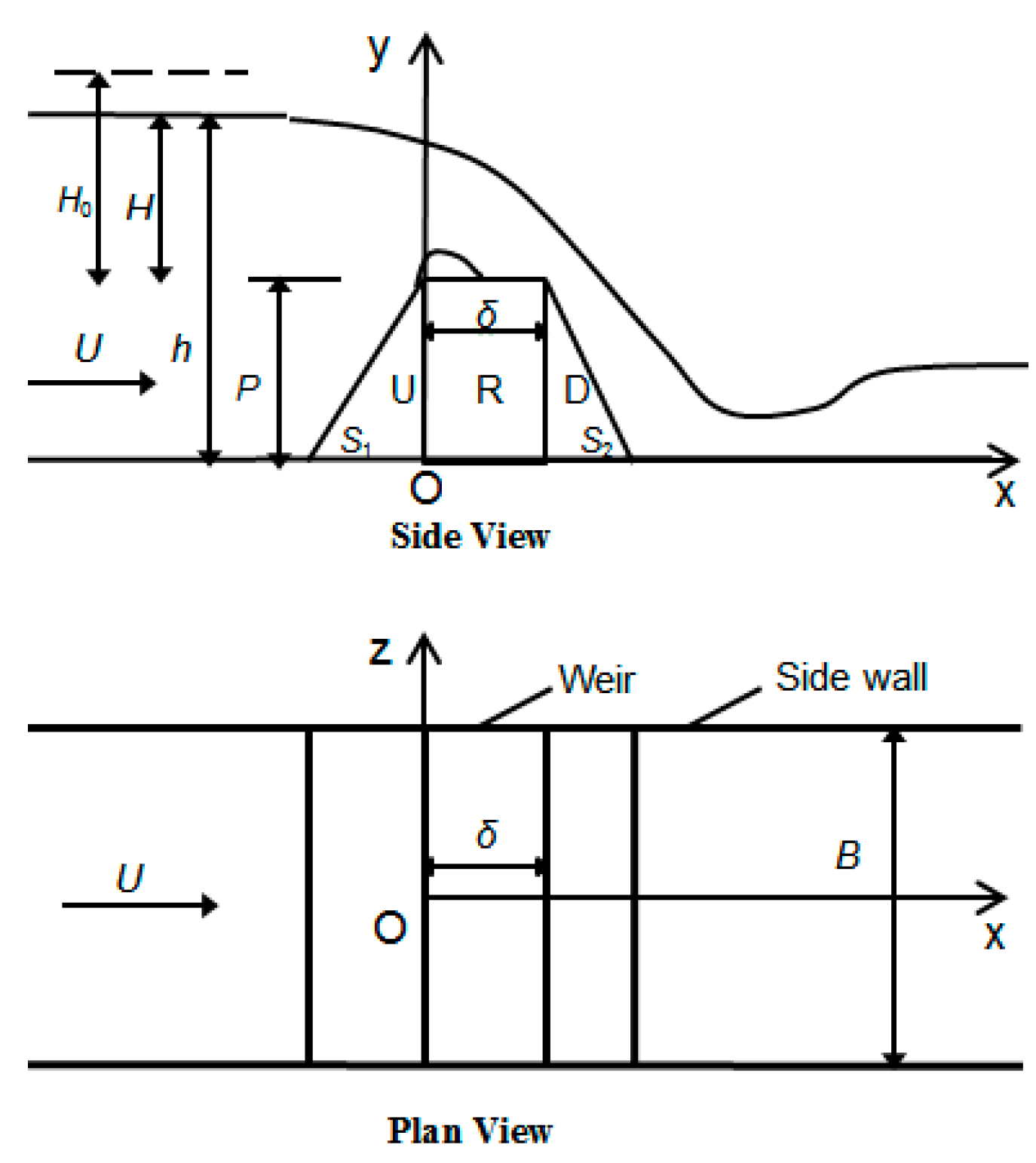
2. Theoretical Analysis of Influential Factors of Discharge Coefficient

Figure 1 showed the definition sketch of short-crested weir constructed from three parts in the longitudinal cross-section: the upstream weir face U, the rectangular crest R and the downstream weir face D. The axis of x and y were along the longitudinal direction and vertical direction, respectively. The weir width B was equal to the flume width without considering lateral contraction. The common practice to determine discharge coefficient in most discharge measuring structures is based on the method of dimensional analysis. The discharge coefficient of the short-crested weir depends on hydraulic conditions, geometrical parameters and fluid properties [24]. Considering these influential factors one could end up with the following relation:

$$F(Q,H_0,B,\delta ,P,S_1,S_2,g,\sigma ,\rho ,\mu )=0$$

(1)

where Q is inflow discharge, m³/s; H₀ is total energy head over crest, H₀ = H + U²/2g, m; U is the approaching velocity, m/s; B is the width of weir, m; δ is the length of weir crest, m; P is the height of weir, m; S₁ and S₂ are up- and downstream slope coefficients, respectively; g is gravity acceleration, m/s²; σ is surface tension of fluid, N/m; ρ is mass density of fluid, kg/m³; μ is dynamic viscosity of fluid, Pa·s. Based on Buckingham’s Π theorem, the three variables of H₀, g and ρ are selected as the basic dimensions, and the relations between dimensionless numbers could be expressed as follows:

$$\frac{Q}{B\sqrt{2g}{H}_0^{3/2}}=f\left(\delta /H_0,P/H_0,S_1,S_2,{\rho }^{0.5}{g}^{0.5}{H}_0/{\sigma }^{0.5},\rho g^{0.5}{H}_0{}^{1.5}/\mu \right)$$

(2)

The left term represents the fundamental weir formulae (Equation (3)) where m is the discharge coefficient.

$$m=\frac{Q}{B\sqrt{2g}{H}_0^{3/2}}$$

(3)

The first four terms on the right of Equation (2) describe the effect of the geometrical properties on the discharge capacity, while the last two terms respectively describe the effects of surface tension and viscosity on the discharge capacity. Isaacs [25] and Ranga Raju et al. [26] concluded that the influence of viscosity and surface tension on the water flowing through weirs could be ignored if the flow depth over the crest was greater than 5.0 cm. Regarding the above conclusion the experiments select the flow depths over the crest between 8.0 cm and 24.0 cm. Regardless of the influence of surface tension and viscosity, Equation (2) is simplified as:

$$m=f_1\left(\delta /H_0,P/H_0,S_1,S_2\right)$$

(4)

Four dimensionless numbers are included in Equation (4): π₁ = δ/H₀, π₂ = P/H₀, π₃ = S₁ and π₄ = S₂, which show the effects of the geometrical parameters and hydraulic conditions on the discharge coefficient of short-crested weir. A good deal of research has studied the influence of weir crest length and weir height on discharge coefficient in detail, so in this study the two elements are settled as constants and the research only focuses on the effect of varying upstream and downstream slope coefficients on discharge coefficient of short-crested weir.

3. Numerical Modeling

A brief introduction to the numerical models is given below, including governing equations, grids layout, and the calculation of the free water surface.

3.1. Governing Equations

In the Cartesian coordinate system, the incompressible continuity (5) and Reynolds-Averaged Navier–Stokes (RANS) (6) equations are used to solve the water motion for turbulent flow.

$$\frac{\partial \overline{u_{\mathrm{i}}}}{\partial x_{\mathrm{i}}}=0$$

(5)

$$\frac{\partial \overline{u_{\mathrm{i}}}}{\partial t}+\overline{u_{\mathrm{j}}}\frac{\partial \overline{u_{\mathrm{i}}}}{\partial x_{\mathrm{j}}}=f_{\mathrm{i}}-\frac{1}{\rho }\frac{\partial \overline{p}}{\partial x_{\mathrm{i}}}+\frac{1}{\rho }\frac{\partial }{\partial x_{\mathrm{j}}}(\mu \frac{\partial \overline{u_{\mathrm{i}}}}{\partial x_{\mathrm{j}}}-\rho \overline{u_{\mathrm{i}}^{\prime }{u}_{\mathrm{j}}^{\prime }})$$

(6)

where $\overline{u_i}$ and $\overline{u_{\mathrm{j}}}$ are average velocity components, m/s; x_i and x_j are Cartesian coordinate axes; f_i is body force, m/s²; p is pressure, Pa; $-\rho \overline{u_{\mathrm{i}}^{\prime }{u}_{\mathrm{j}}^{\prime }}$ is the term of Reynolds shear stress with i, j = 1, 2, 3. In this study, the turbulence is predicted by the renormalization group (RNG) κ-ε turbulent model (turbulent kinetic energy κ and its dissipation ratio ε) [27]. This model could dispose of the high shear and curvature area with higher accuracy and showed better performance in the simulated area with flow separation [28,29]. The wall function method was used for the flow close to the wall and the flow with the lower Reynolds number.

3.2. Disposal of Free Water Surface

In this study, the Volume of Fluid (VOF) method proposed by Hirth et al. [30] is used to accurately predict the variation of the free water surface. The transport Equation (7) of fluid fraction is expressed as follows:

$$\frac{\partial F}{\partial t}+\frac{\partial \left(\overline{u_{\mathrm{i}}}F\right)}{\partial x_{\mathrm{i}}}=0$$

(7)

where F is the fraction of fluid in a cell. This is a two-phase approach where fluid and air are simulated in a structured grid of the finite difference algorithm. The method is based on the concept that every cell has a fraction of fluid (F), which is 0 when the element is full of air and 1 when the element is totally full of fluid. If the value is between 0 and 1, the element contains the free fluid surface.

3.3. Boundary Conditions

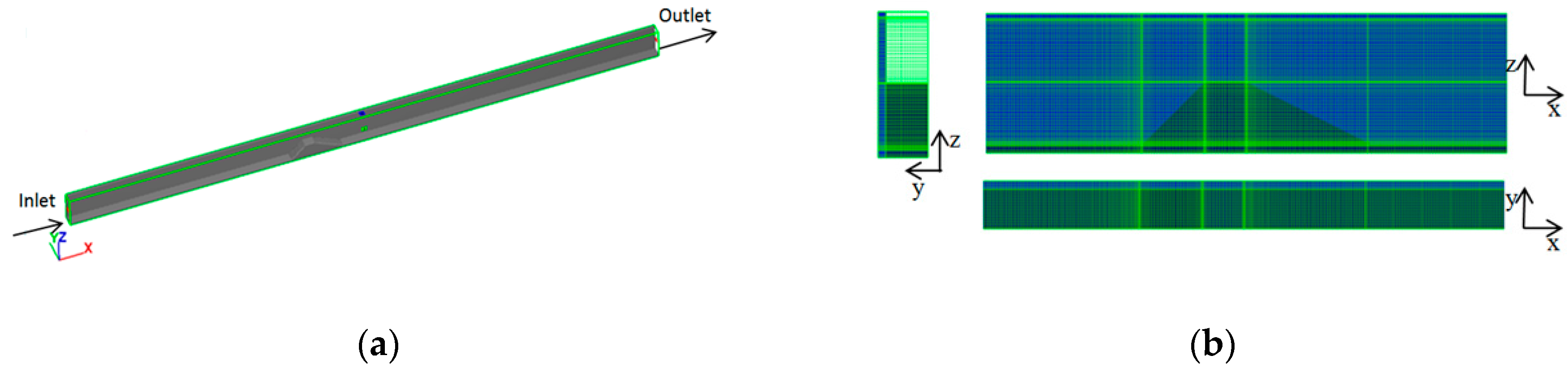
In this study, the laboratory experiments were conducted in order to validate the Computational Fluid Dynamics (CFD) model results. Thus, the boundary conditions in numerical models should consist with the real boundaries in laboratory experiments. Stagnation pressure is used as inflow and outflow boundary, and the corresponding flow depths are specified respectively. Moreover, keep the outflow depth as low as possible to ensure the tail water will not influence the upstream inflow. In view of the symmetry of the weir model and the existence of free surface, the symmetry boundary conditions are set at the symmetrical face and on the top of the flume, respectively. All the solid walls—including the side wall and the flume bed—are considered as the no-slip wall boundary conditions. Moreover, the initial fluid level is specified to save the computational time.

3.4. Grids Layout

The gridding of computational field was shown in Figure 2. The whole computational domain was gridded by nonuniform mesh blocks consisting of rectangular elements. In

Table 1. Gridding characteristics, RMSE and MAPE for the simulated profiles of free surface.

Meshing	Number of Cells	RMSE	MAPE
1	195,600	8.30%	7.53%
2	283,360	6.21%	4.97%
3	568,800	2.93%	0.57%
4	652,500	2.75%	0.45%

the gridding characteristics of numerical models for free surface profiles were provided. To check the accuracy of numerical model the statistical variables of the Root Mean Square Error (RMSE) and the Mean Absolute Percent Error (MAPE) were calculated using the following equations:

$$RMSE\%=100\times \sqrt{\frac{1}{N}{\displaystyle \sum _{i=1}^N{(R_{\mathrm{m}}-R_{\mathrm{s}})}^2}}$$

(8)

$$MAPE\%=\frac{100}{N}{\displaystyle \sum _{\mathrm{i}=1}^N\left|\frac{R_{\mathrm{m}}-R_{\mathrm{s}}}{R_{\mathrm{m}}}\right|}$$

(9)

where R_m and R_s are the laboratory results and simulated results, respectively.

As shown in Table 1, the differences between the results of meshing 3 and meshing 4 were negligible and gridding 3 was chosen. Therefore, the whole computational domain was gridded by 632, 18, 50 rectangular elements in the direction X, Y and Z, respectively. Moreover, the number of grids in x and z direction will be adjusted properly according to the geometry of the weir model and the upstream water depth.

3.5. Numerical Simulation

In this study, the flume with a length of 10.0 m, width of 0.3 m, and height of 0.5 m was defined. The weir model was located at a distance of 4.0 m from the inlet. In

Table 2. List of design schemes of numerical simulation.

Configuration	Scheme	Upstream Side Slope Coeff. S1	Downstream Slope Coeff. S2	No. of Models	Interpretation
VRV	Mij i = 1, j = 1	0.0	0.0	1	Rectangular short-crested weir
URV	Mij i ≠ 1, j = 1	0.3, 0.5, 0.8, 1.0, 1.5, 2.0	0.0	6	Only study the effect of the varying S1 on the discharge coefficient of rectangular short-crested weir
VRD	Mij i = 1, j ≠ 1	0.0	0.4, 0.8, 1.0, 1.3, 1.5, 1.8, 2.0, 3.0	8	Only study the effect of the varying S2 on the discharge coefficient of short-crested weir
URD	Mij i ≠ 1, j ≠ 1	0.3, 0.5, 0.8, 1.0, 1.5, 2.0	0.4, 0.8, 1.0, 1.3, 1.5, 1.8, 2.0, 3.0	48	Study the combinational effect of the varying S1 and S2 on discharge coefficient of rectangular short-crested weir

, the schemes of numerical simulation were listed. The schemes were expressed as M_ij, in which i = 1–7 correspond to seven simulated upstream slope coefficients S₁ of V, 0.3H:1V, 0.5H:1V, 0.8H:1V, 1.0H:1V, 1.5H:1V and 2.0H:1V respectively, while j = 1–9 correspond to nine downstream slope coefficient S₂ of V, 0.4H:1V, 0.8H:1V, 1.0H:1V, 1.3H:1V, 1.5H:1V, 1.8H:1V, 2.0H:1V and 3.0H:1V—all with effective square edges at the joins. Based on the definition of the short-crested weir by Tong et al. [10] the short-crested weir was limited to

$$0.67<\delta /H\le 1.5~2.0,0.5\le P/H<3.0$$

(10)

According to the above criteria, the height of weir P, the length of weir δ and the width of weir B were constant during this study and the values are 24.0 cm, 16.0 cm and 30.0 cm, respectively. There were 63 weir models in total, and each weir model was calculated corresponding to five total energy heads H₀ of 8.0 cm, 12.0 cm, 16.0 cm, 20.0 cm, and 24.0 cm over the crest. The discharge coefficients of the numerical results could be obtained according to Equation (3).

4. Results and Discussion

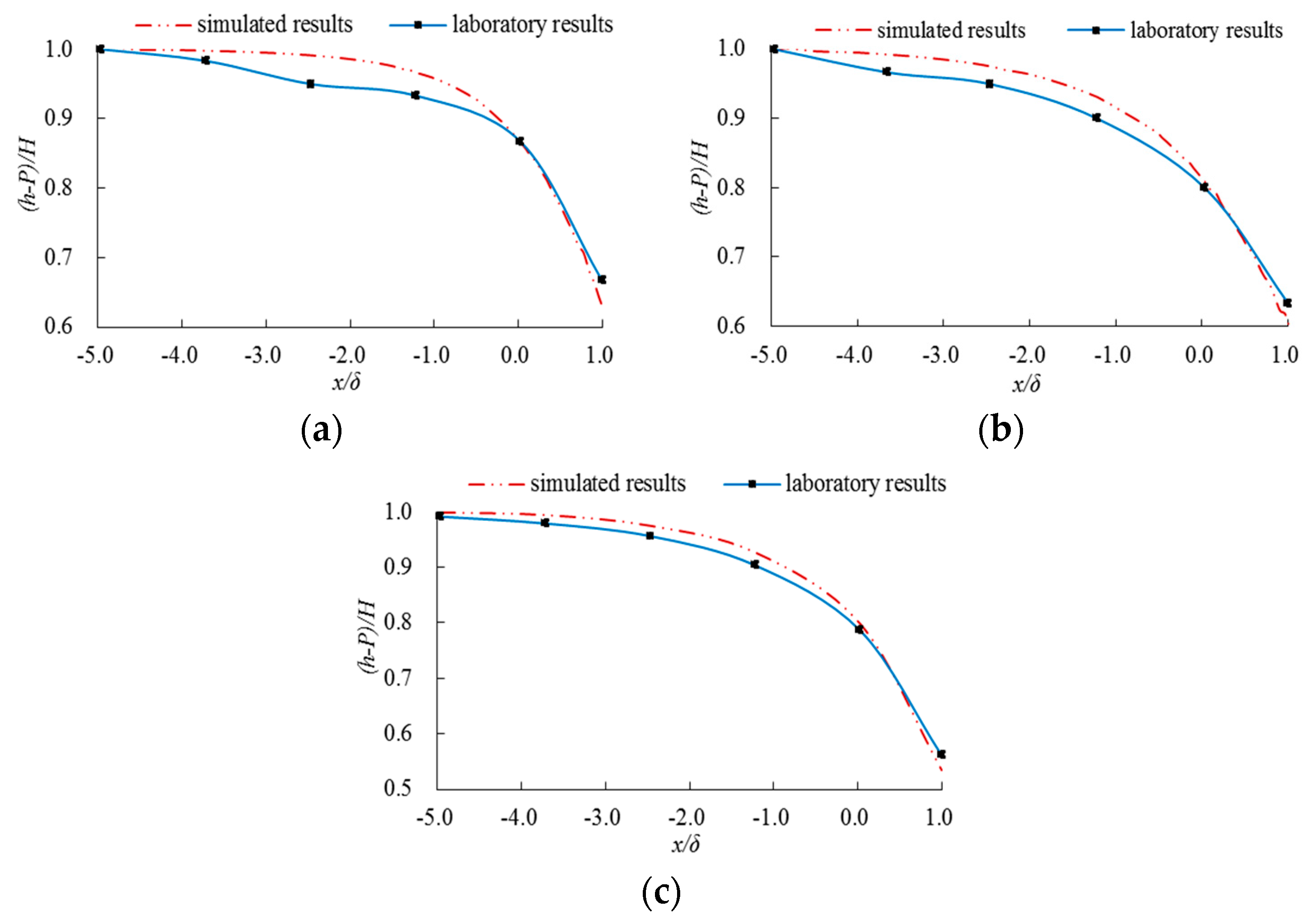
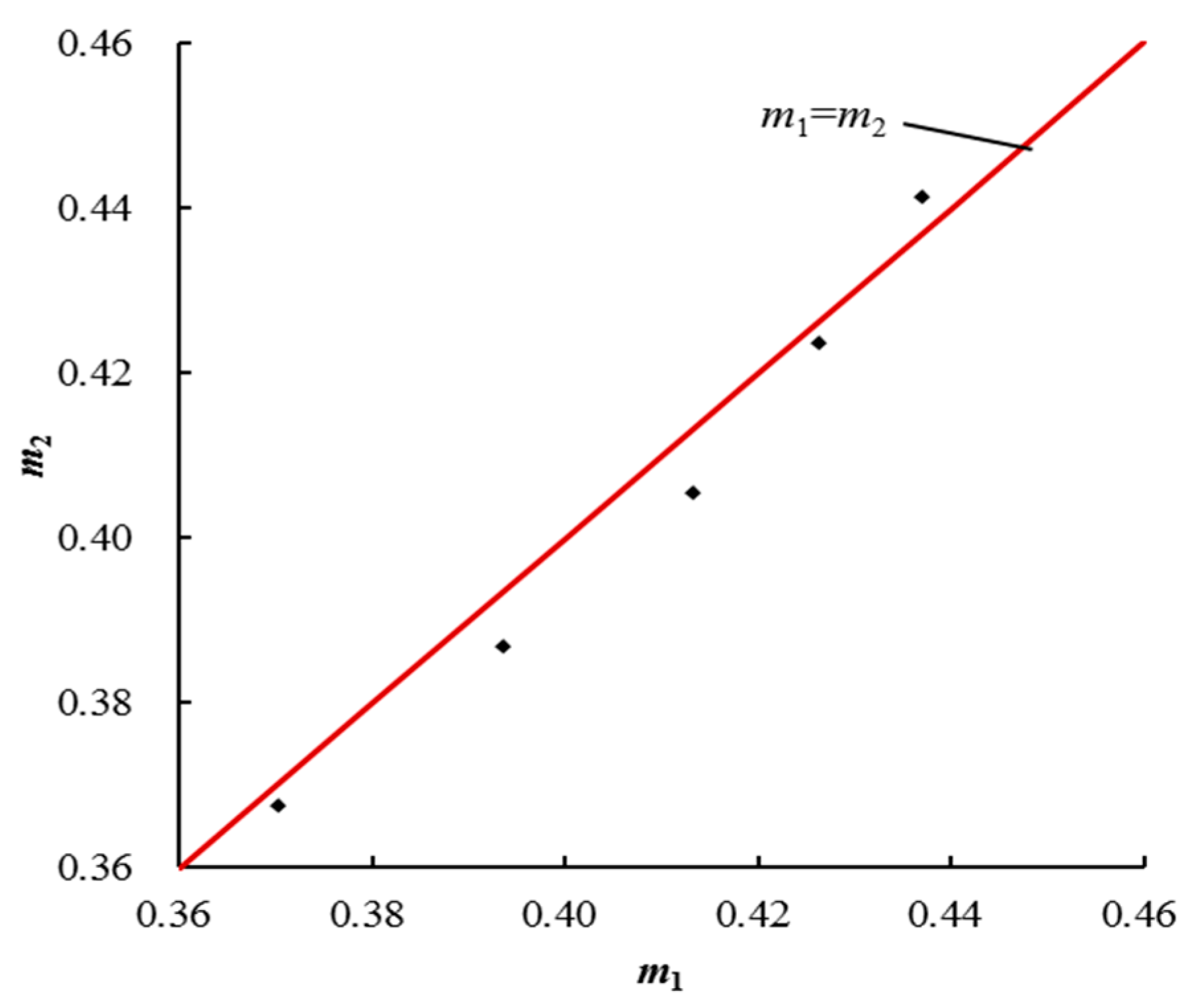
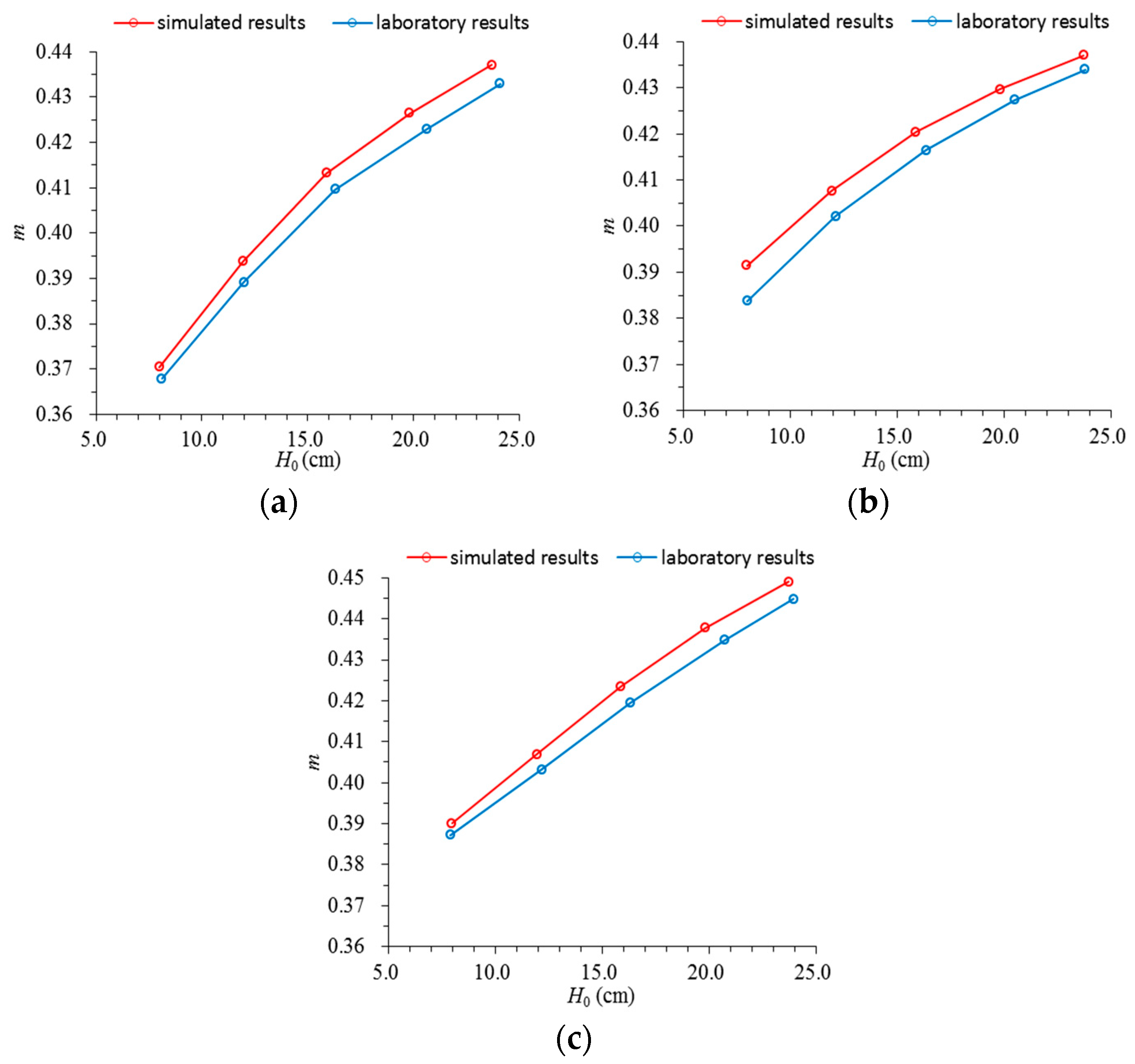
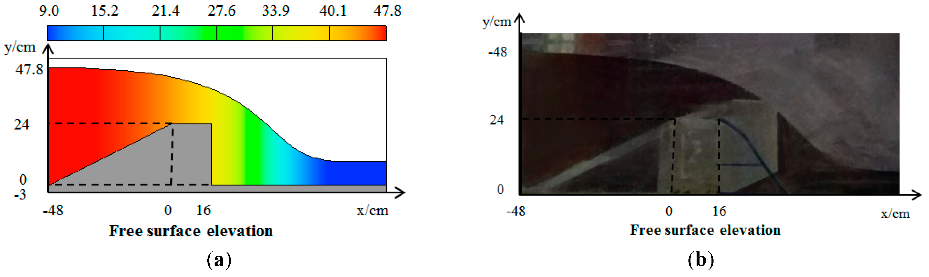
4.1. Validation of Numerical Models

To validate the numerical model results, the laboratory experiments were conducted. The physical model consisted of a self-circular, horizontal, rectangular flume with a short-crested weir. The side walls and weirs were made of Plexiglas. The upstream water level was measured with an accuracy of ±0.1 mm using a needle water level gauge and the volume flow rate with ±0.1 mm using 90° V-notch weir. The tail water depth was selected in a way that would not affect the incoming flow.

Table 3. Range of variables for laboratory measurements.

Scheme	Upstream Slope Coeff. S1	Downstream Slope Coeff. S2	Weir Height P (cm)	Crest Length δ (cm)	Weir Width B (cm)	Total crest Head H0 (cm)
M11	0.0	0.0	24.0	16.0	30.0	8.0, 12.0, 16.0, 20.0, 24.0
M71	2.0	0.0
M73	2.0	0.8

listed the selected geometrical and hydraulic characteristic parameters used to validate the accuracy of the numerical models.

The comparison of discharge coefficients between simulated and laboratory results at free overflow condition are shown in Figure 3. The discharge coefficients gradually increase as the total energy head H₀ increases, and the simulated results are slightly larger than those of laboratory results. Figure 4 shows the comparisons of free surface profiles between the simulated and laboratory results, in which the origin locates at the entrance of the weir crest and h is the fluid level along the streamwise direction and ξ = H₀/(P + δ) is the relative total energy head. The deviation from free surface profiles might result from flow separation and the slightly less accurate simulation for the shapely varied free-surface profile. As shown in Figure 5, the changing trend of free surface elevation is nearly identical for simulated and laboratory results and the bottom roll backflow zone simultaneously appear in back of downstream weir face.

Table 4. RMSE and MAPE for discharge coefficients and flow surface profiles.

Statistical Object	ξ	Scheme	RMSE	MAPE
Discharge coefficient	0.2–0.6	S1 = 0.0, S2 = 0.0	0.37%	0.91%
		S1 = 2.0, S2 = 0.0	0.49%	1.11%
		S1 = 2.0, S2 = 0.8	0.36%	0.85%
Free surface profile	0.6	S1 = 0.0, S2 = 0.0	2.95%	2.80%
		S1 = 2.0, S2 = 0.0	2.68%	2.86%
		S1 = 2.0, S2 = 0.8	1.84%	2.20%

lists the RMSE and MAPE for the discharge coefficients and free surface profiles. In consideration of the comparative results it is obvious that the numerical model is able to accurately predict the water surface over the short-crested weir and the directly linked discharge coefficient.

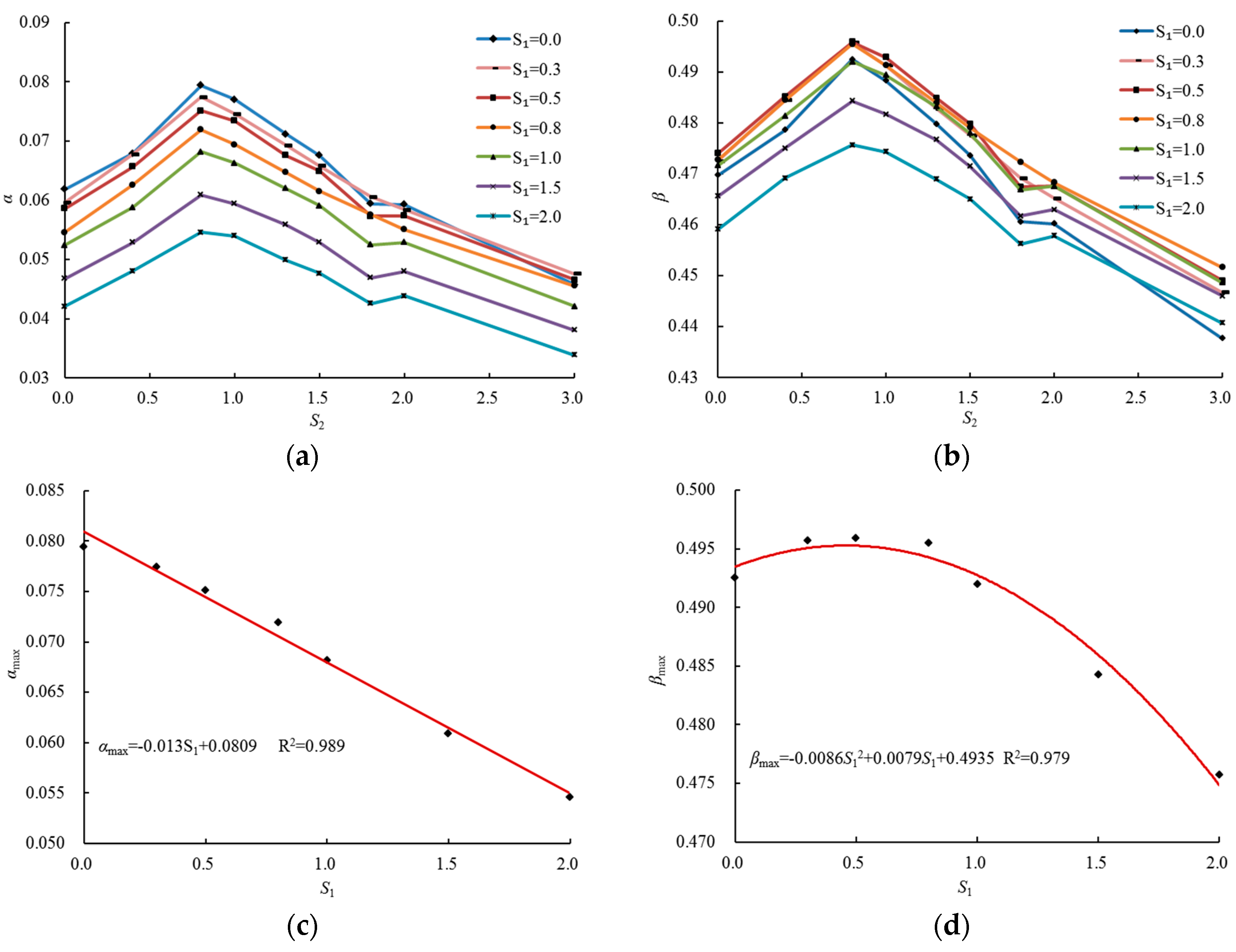
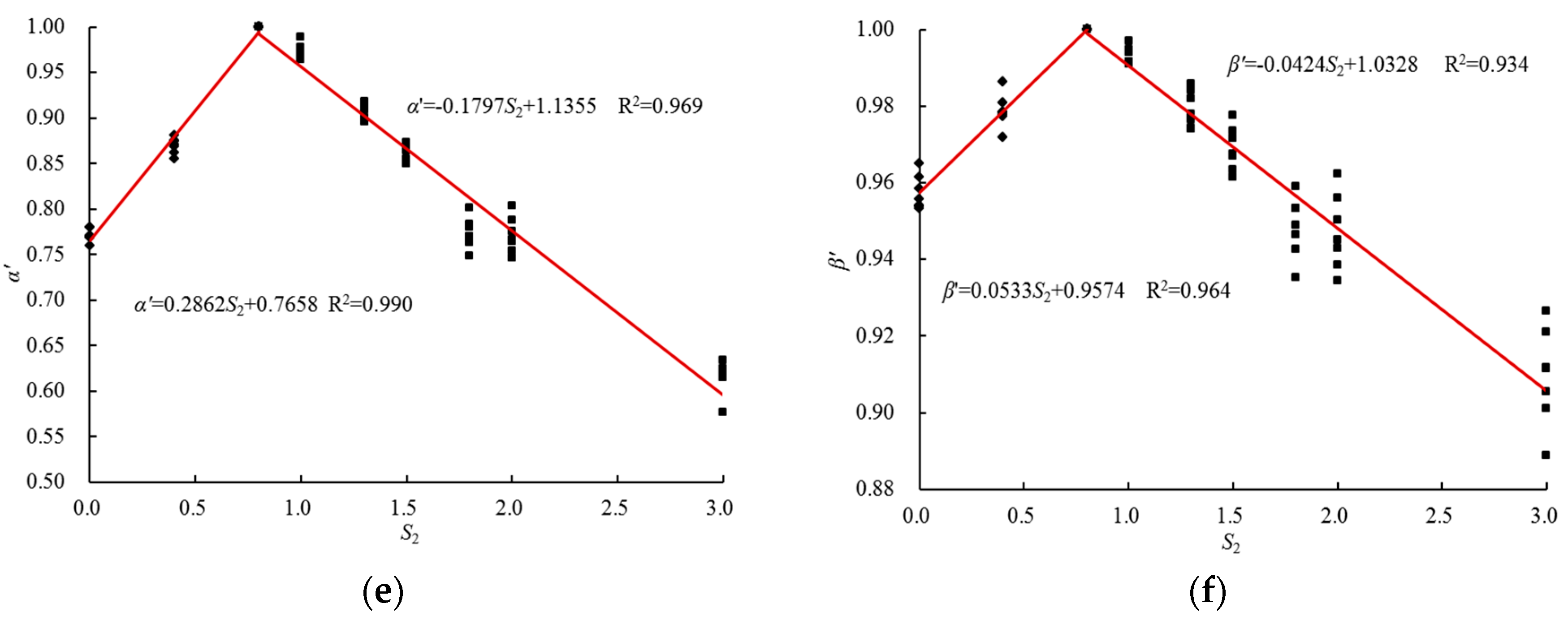
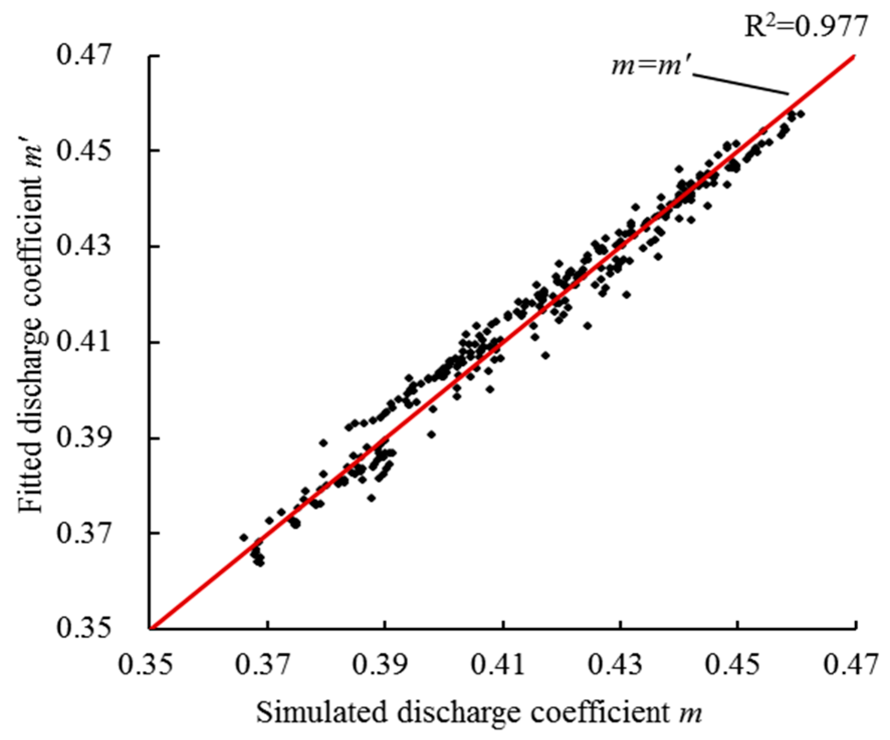
4.2. Calculation Formula of Discharge Coefficient

Sixty-three weir models and 315 numerical simulations are conducted. From the dimensional analysis of Equation (4) a monotonically increasing linear relation between m and lnξ for different weir models is expressed as follows:

$$m\prime =\alpha \ln \left(\frac{H_0}{P+\delta }\right)+\beta$$

(11)

where m′ is the fitted discharge coefficient and α and β are dimensionless parameters determined by S₁ and S₂. In Figure 6a–b the effects of S₂ on α and β are shown for all of the upstream slope coefficients S₁, and the corresponding values are listed in

Table 5. Values of α and β in different combinations of upstream and downstream slope coefficients.

Parameter	Upstream Slope Coefficient	Downstream Slope Coefficient
		S1 = 0.0	S1 = 0.3	S1 = 0.5	S1 = 0.8	S1 = 1.0	S1 = 1.5	S1 = 2.0
α	S2 = 0.0	0.0619	0.0596	0.0586	0.0546	0.0524	0.0468	0.0421
	S2 = 0.4	0.0679	0.0678	0.0657	0.0626	0.0588	0.0529	0.0481
	S2 = 0.8	0.0794	0.0774	0.0751	0.0719	0.0682	0.0609	0.0546
	S2 = 1.0	0.0770	0.0746	0.0734	0.0694	0.0663	0.0594	0.0540
	S2 = 1.3	0.0712	0.0693	0.0676	0.0647	0.0620	0.0559	0.0499
	S2 = 1.5	0.0676	0.0658	0.0649	0.0615	0.0591	0.0529	0.0477
	S2 = 1.8	0.0594	0.0606	0.0573	0.0576	0.0525	0.0469	0.0426
	S2 = 2.0	0.0593	0.0584	0.0574	0.0551	0.0529	0.0480	0.0439
	S2= 3.0	0.0458	0.0476	0.0466	0.0456	0.0421	0.0381	0.0339
β	S2 = 0.0	0.4697	0.4725	0.4740	0.4727	0.4716	0.4656	0.4591
	S2 = 0.4	0.4786	0.4845	0.4852	0.4845	0.4814	0.4750	0.4692
	S2 = 0.8	0.4925	0.4957	0.4959	0.4955	0.4920	0.4843	0.4757
	S2 = 1.0	0.4883	0.4913	0.4929	0.4913	0.4894	0.4817	0.4743
	S2 = 1.3	0.4798	0.4828	0.4849	0.4839	0.4832	0.4767	0.4689
	S2 = 1.5	0.4736	0.4776	0.4798	0.4791	0.4780	0.4715	0.4650
	S2 = 1.8	0.4606	0.4692	0.4674	0.4723	0.4669	0.4617	0.4562
	S2 = 2.0	0.4602	0.4652	0.4676	0.4683	0.4676	0.4630	0.4578
	S2 = 3.0	0.4377	0.4467	0.4490	0.4516	0.4486	0.4460	0.4407

. Both of α and β firstly increase until they reach the maximum of α_max and β_max at S₂ = 0.8, and then decrease until they reach the minimum of α_min and β_min at S₂ = 3.0. Moreover, a good linear relation between α_max and S₁ and a good parabolic relation between β_max and S₁ are shown in Figure 6c,d, and the relations could be expressed as follows:

$${\alpha }_{\max }=-0.013S_1+0.0809$$

(12)

$${\beta }_{\max }=-0.0086S_1{}^2+0.0079S_1+0.4935$$

(13)

with R² = 0.989 and 0.979 respectively. The data are normalized by introducing the variables of α′ = α/α_max and β′ = β/β_max as shown in Figure 6e,f. Both of α′ and β′ have good piecewise linear relations with S₂, which could end up with the expressions:

$$\alpha \prime =\{\begin{array}{ll}0.2862S_2+0.7658& 0.0\le {\mathrm{S}}_2\le 0.8\\ -0.1797S_2+1.1355& 0.8<{\mathrm{S}}_2\le 3.0\end{array}$$

(14)

$$\beta \prime =\{\begin{array}{ll}0.0533S_2+0.9574& 0.0\le {\mathrm{S}}_2\le 0.8\\ -0.0424S_2+1.0328& 0.8<{\mathrm{S}}_2\le 3.0\end{array}$$

(15)

Combining Equations (12)–(15), the calculation formula of discharge coefficient of rectangular short-crested weir with varying upstream and downstream slope coefficients (URD) is derived as Equation (11), where

$$\alpha =\{\begin{array}{ll}\left(-1.3S_1+8.09\right)\left(2.862S_2+7.658\right)\times {10}^{-3}& 0.0\le S_1\le 2.0,0.0\le S_2\le 0.8\\ \left(-1.3S_1+8.09\right)\left(-1.797S_2+11.355\right)\times {10}^{-3}& 0.0\le S_1\le 2.0,0.8<S_2\le 3.0\end{array}$$

(16)

$$\beta =\{\begin{array}{ll}\left(-8.6S_1^2+7.9S_1+493.5\right)\left(5.33S_2+95.74\right)\times {10}^{-5}& 0.0\le {\mathrm{S}}_1\le 2.0,0.0\le S_2\le 0.8\\ \left(-8.6S_1^2+7.9S_1+493.5\right)\left(-4.24S_2+103.28\right)\times {10}^{-5}& 0.0\le {\mathrm{S}}_1\le 2.0,0.8<S_2\le 3.0\end{array}$$

(17)

The Equation (11) is valid for 0.0 ≤ S₁ ≤ 2.0, 0.0 ≤ S₂ ≤ 3.0, 0.67 ≤ δ/H ≤ 2.0, 1.0 ≤ P/H ≤ 3.0 and −1.61 ≤ lnξ ≤ −0.51. The range out of simulated results should be verified further. The deviation from m is plotted in Figure 7. The RMSE, MAPE and R² for discharge coefficient are computed with the values 0.36%, 0.02% and 0.977, respectively. Recently, it has not have a discharge coefficient formula including S₁ and S₂. The discharge coefficient m₁ calculated by Equation (11) at S₁ = 0 and S₂ = 0 is compared with the Equation (18) proposed by Govinda Rao and Muralidhar [1], and comparative results are shown in the Figure 8 with the maximum relative error 1.92%.

$$m_2=0.08\frac{H}{\delta }+0.329$$

(18)

The application range of Equation (18) is 0.4 ≤ H/δ ≤ 1.5–1.9. Analyzing Equation (11) concludes that the geometrical configuration corresponding to the maximum discharge coefficient relates closely to the value range of lnξ. In the range −1.06 < lnξ ≤ −0.51 (13.8 cm < H₀ ≤ 24 cm), m′ reaches m′_max = (7.43lnξ + 49.53) × 10⁻² at S₁ = 0.459 − 0.75lnξ and S₂ = 0.8; in the range −1.61 ≤ lnξ ≤ −1.06 (8.0 cm ≤ H₀ ≤ 13.8 cm), m′ reaches m′_max = (5.46lnξ + 47.49) × 10⁻² at S₁ = 2.0 and S₂ = 0.8. And the maximum discharge coefficient is always obtained at S₂ = 0.8. The existence of a maximum discharge coefficient at S₂ = 0.8 relates to the flow regime in back of downstream weir face. Comparisons of the velocity fields and free-surface elevations of weirs at S₁ = 1.0 with H/δ = 1.41 for S₂ = 0.0, 0.8 and 2.0 are shown in Figure 9 and Figure 10, respectively. In Figure 9a, a bottom roll backflow zone forms between the downstream weir face and the nappe at S₂ = 0.0, and air is entrained into it simultaneously. The backflow will lift the nappe, resulting in the rise of downstream free surface profile, and reduce the discharge capacity. Moreover, the outline of backflow zone roughly forms an isosceles triangle on the side view, which is identical to the test observation. In Figure 9b, the backflow zone disappears and the downstream free surface profile falls after a rise at S₂ = 0.8 compared with the weir at S₂ = 0.0. In this situation the nappe attached on the weir face perfectly, which improves the discharge capacity. With increasing S₂, the reattachment point produced by the combined action of inertial force and gravity is gradually covered by the downstream weir side, and the downstream free surface profile is lifted higher by the weir face than the weir at S₂ = 0.0 as shown in Figure 9c and Figure 10.

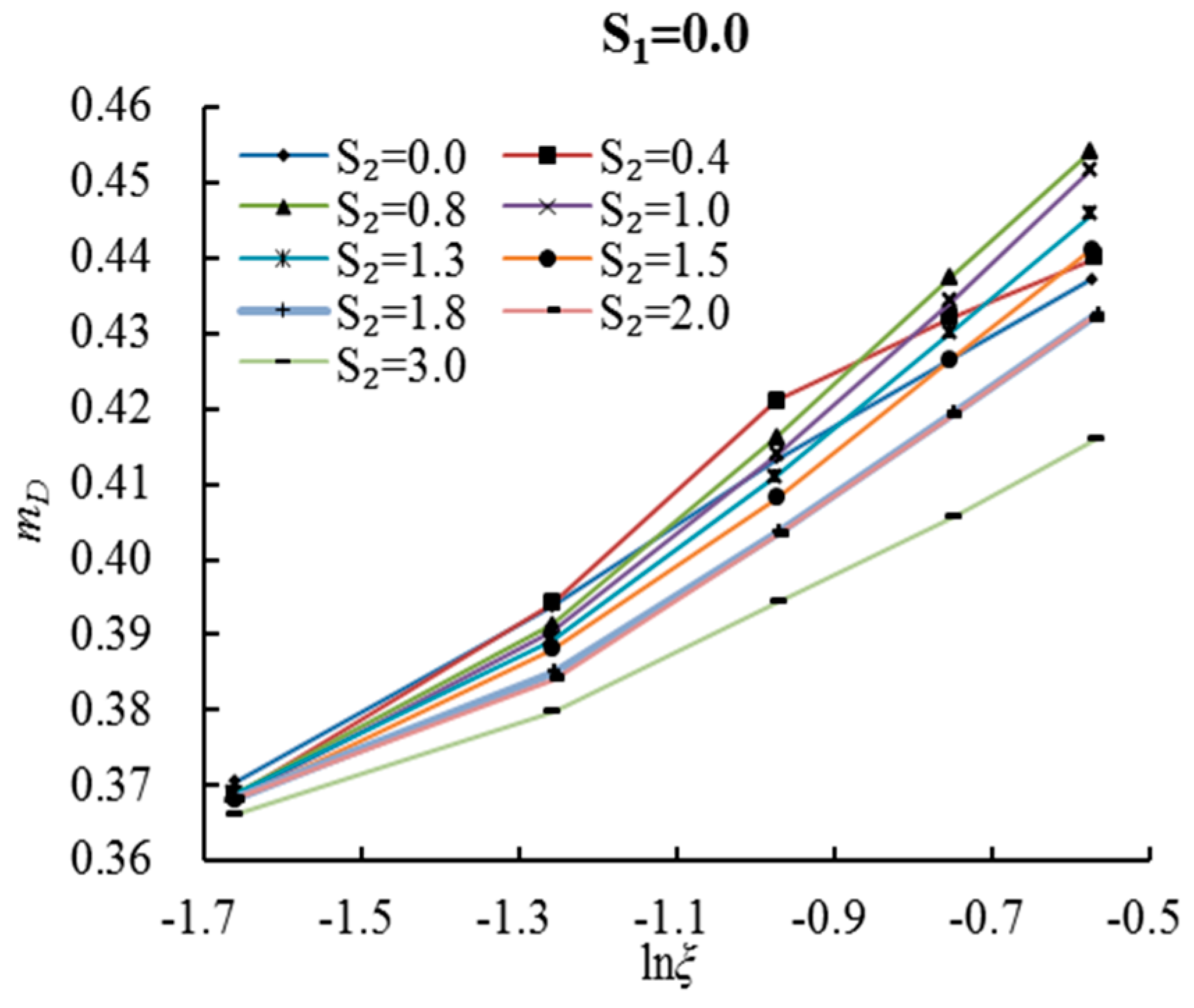
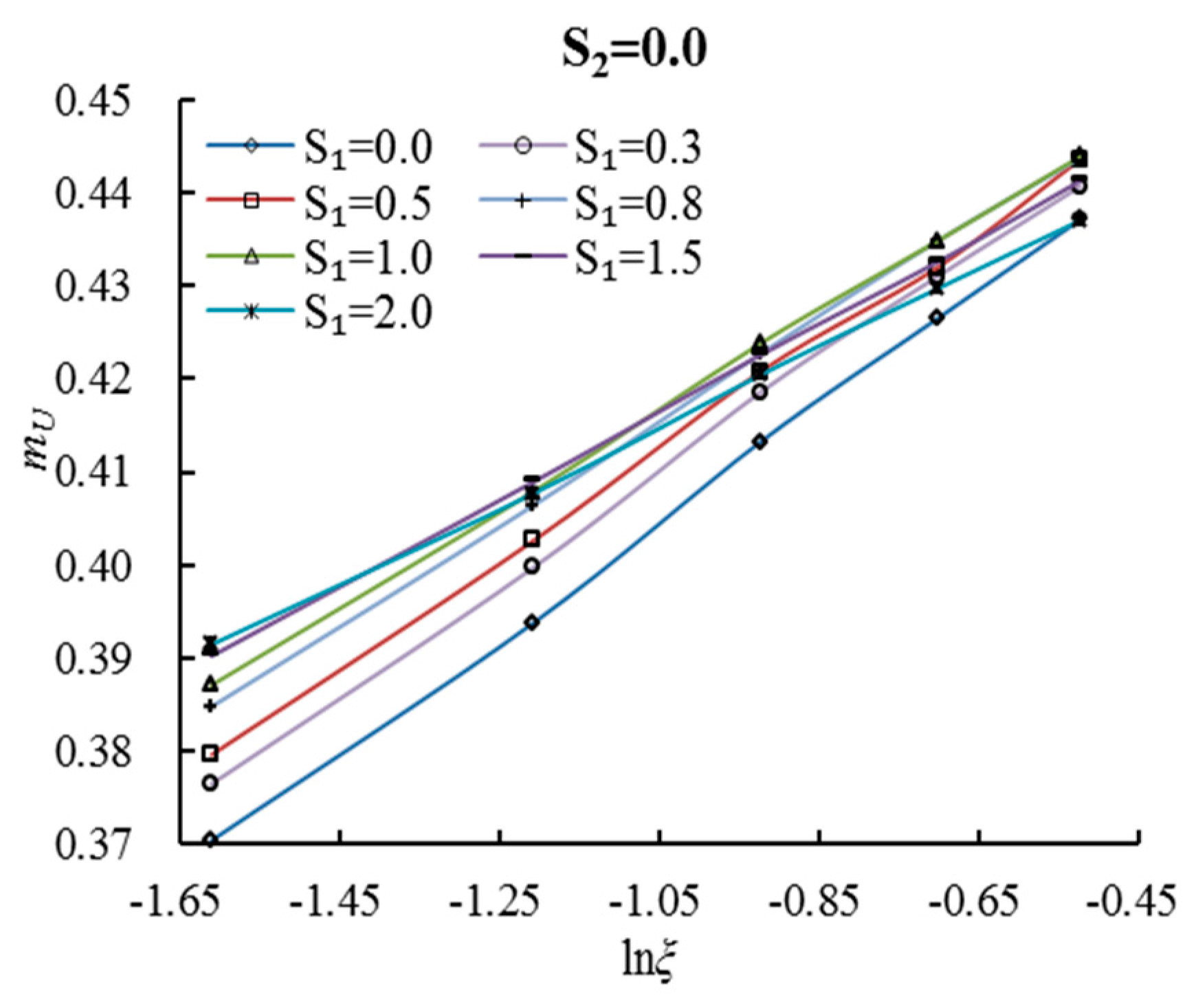
4.3. Effects of Slope Coefficients on Discharge Coefficient

When S₂ = 0.0, Equation (11) would be simplified as:

$$m_{\mathrm{U}}\prime =\left[\left(-0.9991S_1+6.2172\right)\ln \xi -0.8234S_1^2+0.7563S_1+47.2477\right]\times {10}^{-2}$$

(19)

where m_U′ is the fitted discharge coefficient for S₂ = 0.0. Analyzing the fitted equation indicates that for a given lnξ, m_U′ firstly increases until it reaches the maximum at S₁ = 0.5822 − 0.7055lnξ, and then decreases with S₁.

In Figure 11, the difference in discharge coefficients for different values of S₁ shows a decreasing trend with increasing lnξ. In view of energy conservation law, the difference is produced by the frictional head loss of h_f and local head loss of h_j in the progress of free overflow. When lnξ holds constant, the gradually slowing upstream slope increases the flow run and reduces the streamline curvature of inflow, accordingly h_f is increasing and h_j is decreasing. In this progress, the increment of the former is less than the decrement of the latter, so m_U′ continues increasing till S₁ = 0.5822 − 0.7055lnξ. When the upstream slope continued slowing, the increment of h_f exceeds the decrement of h_j, so the discharge coefficient is gradually decreasing. With increasing total energy head of H₀ over the crest the difference in the total head loss of h_w where h_w = h_f + h_j is gradually decreasing, so the difference in discharge coefficients is gradually decreasing for different values of S₁.

When S₁ = 0.0, Equation (11) would be simplified as:

$$m_D\prime =\{\begin{array}{ll}\left[\left(2.315\ln \xi +2.63\right)S_2+6.195\ln \xi +47.248\right]\times {10}^{-2}& 0.0\le S_2\le 0.8\\ \left[-\left(1.454\ln \xi +2.09\right)S_2+9.186\ln \xi +50.969\right]\times {10}^{-2}& 0.8<S_2\le 3.0\end{array}$$

(20)

where m_D′ is the fitted discharge coefficient for S₁ = 0.0. It reveals that the maximum of discharge coefficient m_D′_max depends on both of S₂ and ξ. In the range −1.29 < lnξ ≤ −0.51, m_D′ reaches the maximum of m_D′_max = (7.85lnξ + 49.17) × 10⁻² at S₂ = 0.8; while in the range −1.61 ≤ lnξ ≤ −1.29 it reaches the maximum of m_D′_max = (6.101lnξ + 46.89) × 10⁻² at S₂ = 0.0.

In Figure 12, the difference in discharge coefficients for different values of S₂ shows an increasing trend with increasing lnξ. Similarly, the difference is caused by h_f and h_j, in which the local head loss is mainly produced by inflow dropping into the downstream with forming the bottom roll backflow zone between the downstream weir face and the nappe. Moreover, the size of the backflow zone is proportionate to the local head loss. In the range −1.29 < lnξ ≤ −0.51, increasing S₂ will gradually decrease the size of the backflow zone until it disappears at S₂ =0.8, and the local head loss plays the decisive role in this progress. Continuing increasing S₂, h_f tends to be dominant with increasing flow run. In the range −1.61 ≤ lnξ ≤ −1.29, although the backflow zone cannot be formed due to the lower crest depth, the subpressure zone is formed around the downstream weir face. Smaller the value of S₂ is, larger the maximum of subpressure zone is. Although it increases the discharge coefficient, the instability of subpressure zone can lead to the instability of weir flow. Therefore, the design of short-crested weir should take the downstream slope into consideration.

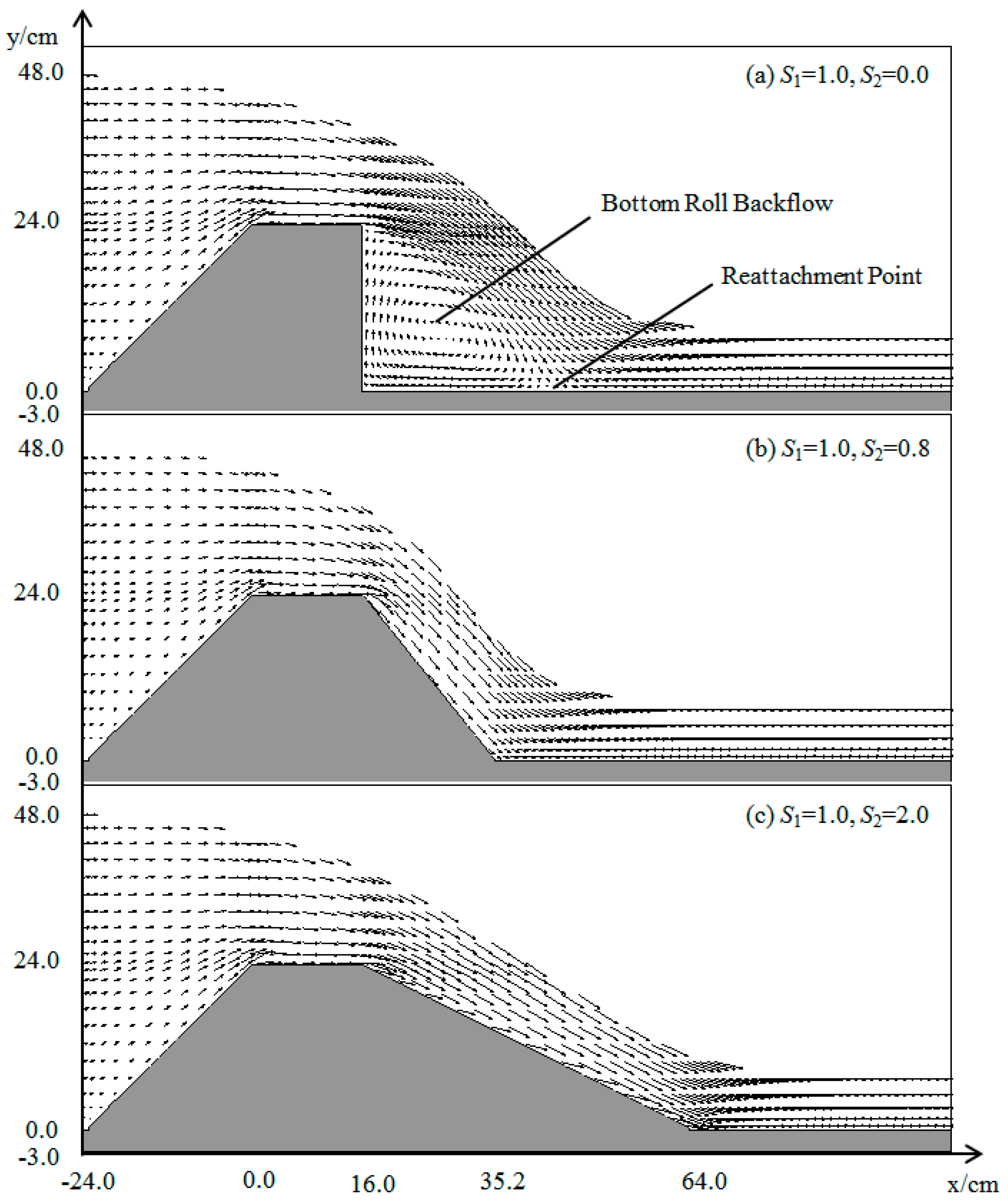
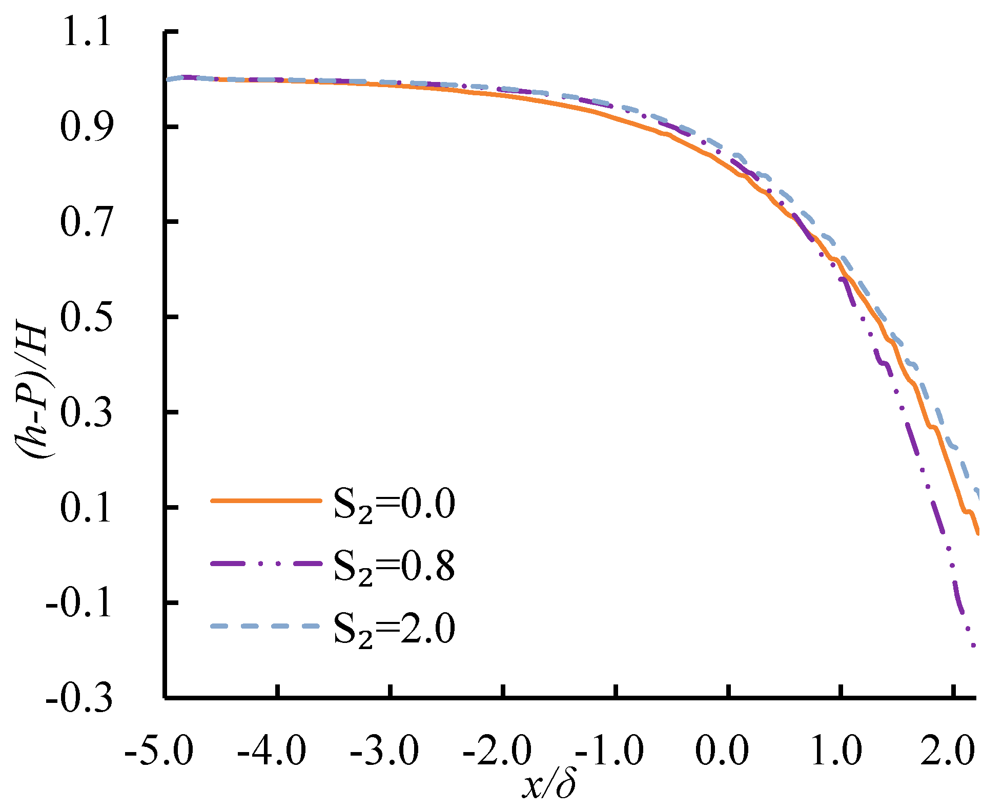
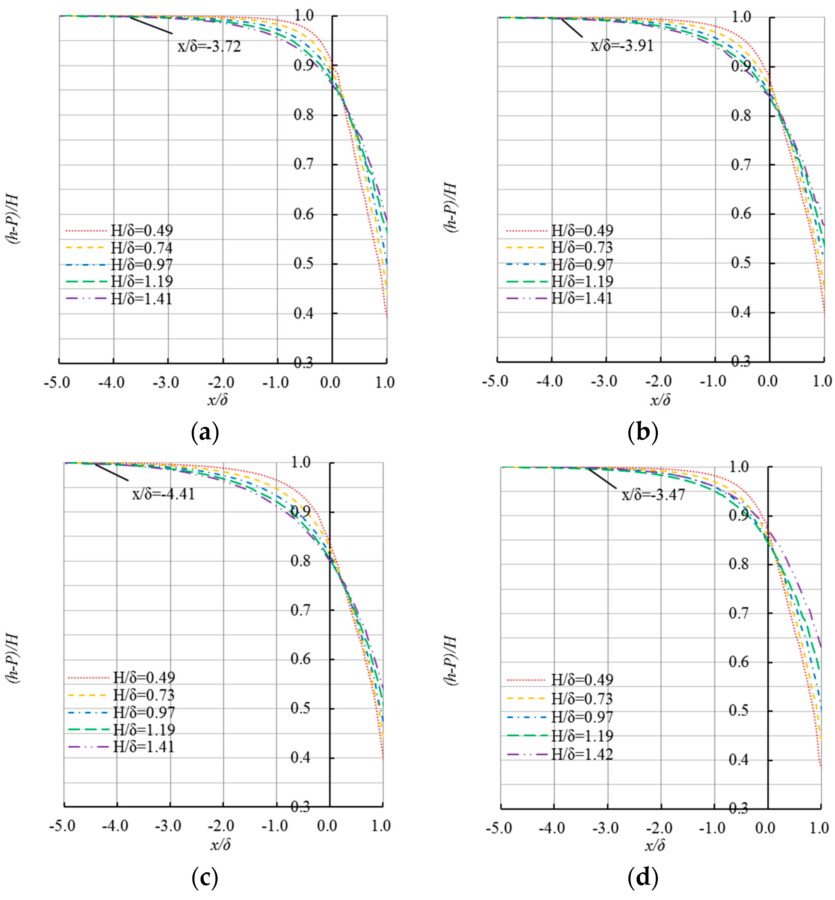
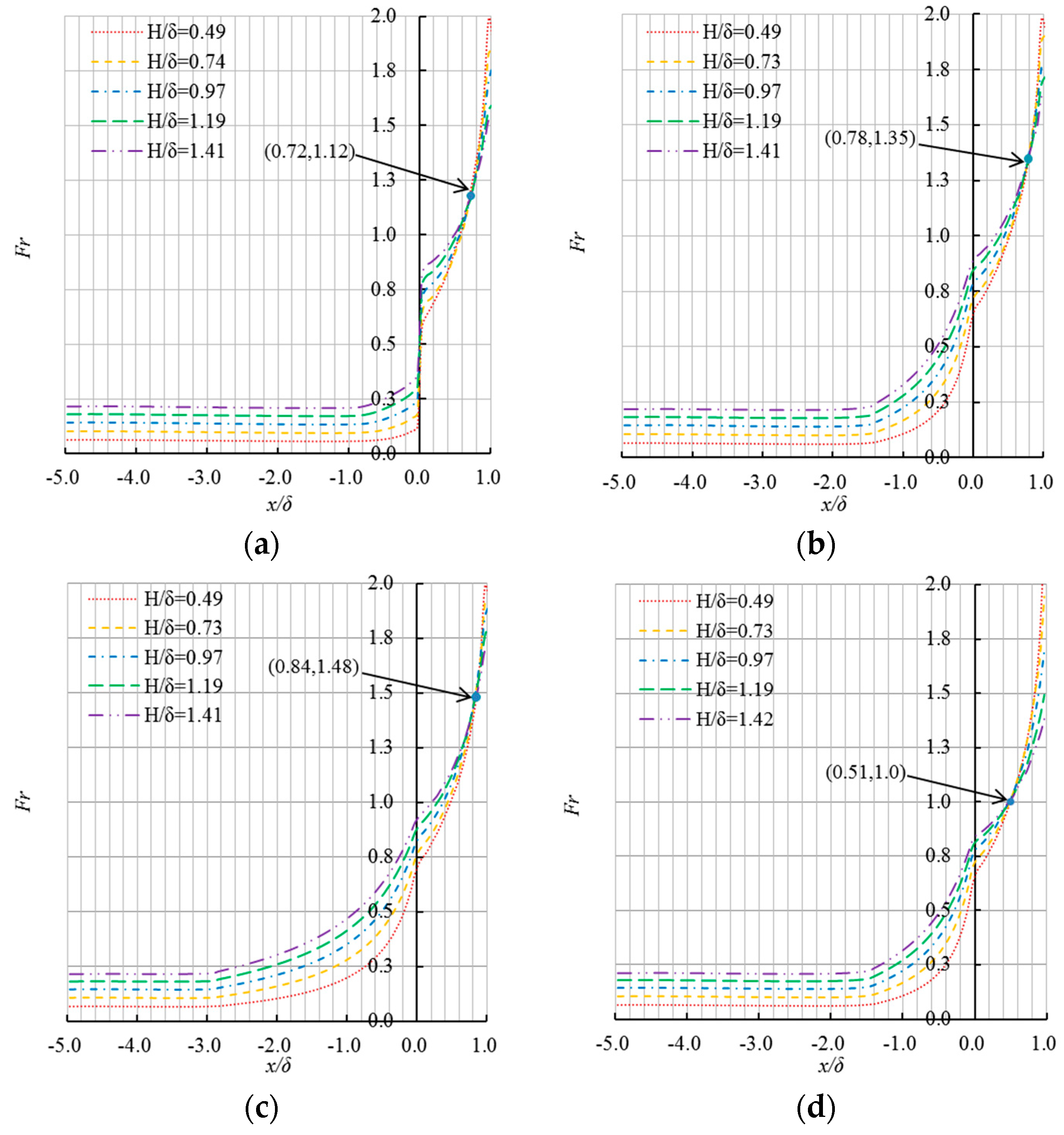
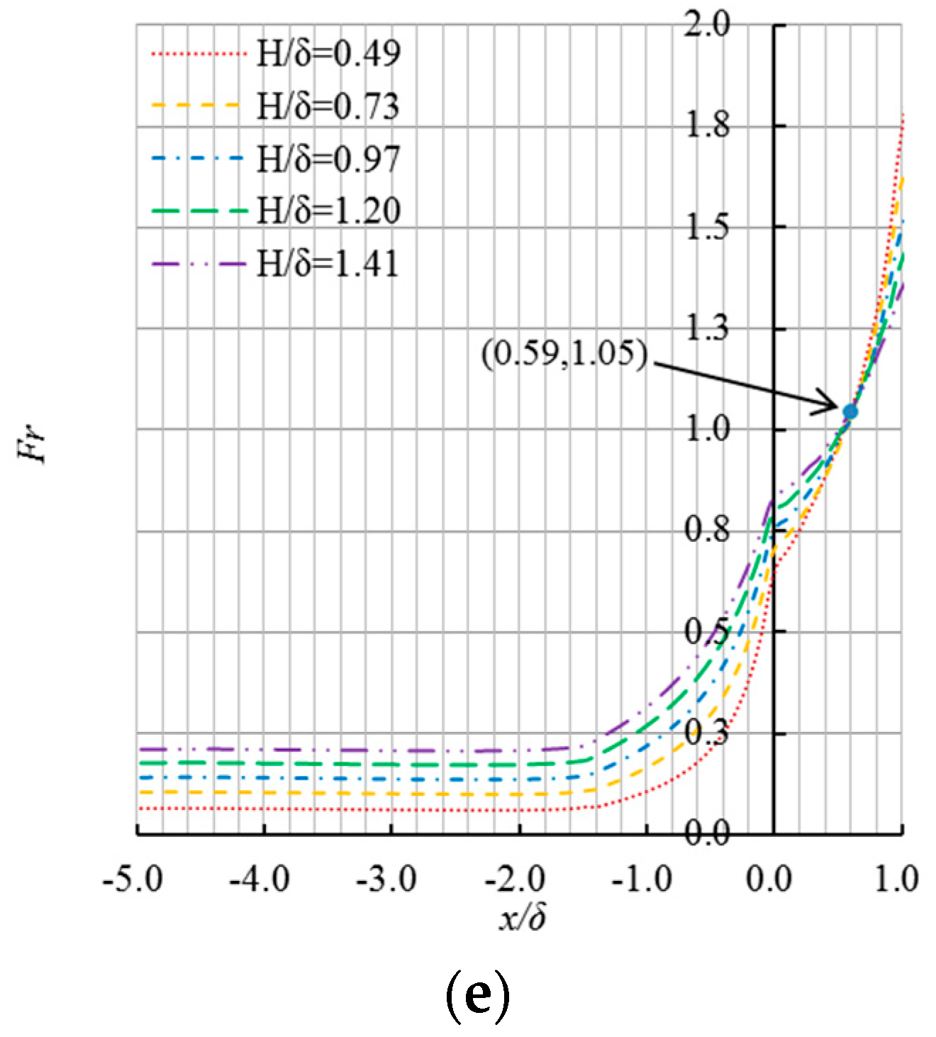
4.4. Effects of Slope Coefficients on Free Surface Profiles

In this numerical study, the variations of free surface profiles and Froude numbers over the crest with various slope coefficients are investigated in overflow conditions. In Figure 13, the normalized free surface elevation of (h − P)/H is plotted against x/δ for different values of H/δ. As shown, the free surface profiles are self-similar. The range of (h − P)/H shows a decreasing trend with growing x/δ in all cases. The free surface profile can be divided into two parts due to the gradient: a slow descending segment and a sharp descending segment. For the former the curvature is nearly 0, but for the latter it descends quickly with hydraulic drop happening. The flow separation phenomenon happening around x/δ = 0.0 (at the entrance of weir crest) produces large energy losses and results in free surface profile descending sharply. Moreover, the range of the curvature of free surface profile shows a decreasing trend with growing H/δ in all cases.

In Figure 14, Fr is plotted against x/δ for different values of H/δ. The range of Fr shows an increasing trend with growing x/δ in all cases. When Fr < 1, the value of F_r for the same x/δ decreases as H/δ decreases, which indicates that for a smaller flow rate, the inertial force on the flow is smaller. Under the action of gravity, the free surface profile is easier to bend, resulting in a more curved surface profile. When Fr > 1, the value of Fr for the same x/δ increases as H/δ decreases, indicating that for a smaller flow rate, the ratio of inertial force to gravity is so large it can keep the higher profile gradient. Moreover, for a given weir model, the position where supercritical flow takes place is relatively rearward as H/δ decreases.

Comparisons of free surface profiles and Fr over the weirs at S₂ = 0.8 for S₁ = 0.0, 1.0 and 2.0 are shown in Figure 13a–c and Figure 14a–c. The plots reveal that increasing S₁ leads to the increase of surface curvature before the crest entrance and the decrease over the crest. When H/δ holds constant, increasing S₁ will accelerate supercritical flow taking place. Analyzing the effect of different S₂ on free surface profiles over crest at S₁ = 1.0 in Figure 13b,d,e and the corresponding Froude numbers in Figure 14, it can be concluded that increasing S₂ leads to the decrease of free surface curvature over the crest and it has no obvious influence on the curvature of free surface profile before the crest entrance.

5. Conclusions

The effects of varying upstream and downstream slope coefficients on discharge coefficients of rectangular short-crested weirs were studied systemically by the combination of laboratory experiments and numerical simulation. A calculation formula was proposed by using the dimensional analysis between hydraulic parameters and geometrical parameters: height of weir, length of weir, upstream overflow total energy head, and upstream and downstream slope coefficients. Moreover, the free surface profiles over the weirs were numerically investigated.

The upstream overflow total energy head played a decisive role on the discharge coefficient of rectangular short-crested weirs. For a certain configuration of a short-crested weir, the discharge coefficient is slightly increased as the total energy head H₀ increases. As H₀ increases, the difference in discharge coefficients for different values of S₁ shows a decreasing trend with increasing lnξ, while the trend is opposite for different values of S₁. For a given total energy head over the crest, the rectangular short-crested weir with varying upstream slope has a convex parabolic relation between S₁ and the discharge coefficient, while the weir with varying downstream slope has a relation of piecewise linearity between the S₂ and the discharge coefficient. For a higher H₀, the maximum discharge coefficient is always obtained at 0.8H:1V of downstream slope.

Increasing the upstream slope coefficients leads to the free surface curvature increasing before the crest entrance and decreasing over the crest, while increasing the downstream slope coefficients leads to the decrease of free surface curvature on the crest. In addition, the structural design for short-crested weirs should take the downstream slope into consideration.

The calculation formula of the discharge coefficient was derived by the nonlinear regression. It is a function of the upstream slope coefficient (S₁), the downstream slope coefficient (S₂), and the ratio of total energy head to the sum of crest length and crest height (H₀/(P + δ)). The RMSE, MAPE and R² for the proposed equation are calculated, and the values are 0.36%, 0.02% and 0.977, respectively.

References

1. Govinda Rao, N.S.; Muralidhar, D. Discharge characteristics of weirs of finite-crest width. La Houille Blanche 1963, 5, 537–545. [Google Scholar] [CrossRef]
2. Li, J.X.; Zhao, Z.X. Hydraulics; Hohai University Press: Nanjing, China, 2001. (In Chinese) [Google Scholar]
3. Inozemtsev, Y.P. Cavitation destruction of concrete and protective facings under natural conditions. Power Technol. Eng. 1969, 3, 35–42. [Google Scholar] [CrossRef]
4. Bos, M.G. Discharge Measurement Structures; NASA Sti/recon Technical Report N; National Aeronautics and Space Administration: Washington, DC, USA, 1989; Volume 78, pp. 120–122.
5. Ramamurthy, A.; Tim, U.; Rao, M. Characteristics of square-edged and round-nosed broad-crested weirs. J. Irrig. Drain. Eng. 1988, 114, 61–73. [Google Scholar] [CrossRef]
6. Tong, H.H.; Lan, F.R. Analysis of the effect of weir height on discharge capacity of low weirs. Yangtze River 2002, 11, 20–21. (In Chinese) [Google Scholar]
7. Singer, J. Square-edged broad-crested weir as a flow measurement device. Water Water Eng. 1964, 68, 229–235. [Google Scholar]
8. Kiselef, P.G.; Zhou, P.; Hua, Z. Hydraulics: Principle of Fluid Mechanics; China Water & Power Press: Beijing, China, 1983. (In Chinese) [Google Scholar]
9. Li, W. Hydraulic Reckoner; China Water & Power Press: Beijing, China, 2006. (In Chinese) [Google Scholar]
10. Tong, H.H.; Ai, K.M.; Ding, X.Q. Discharge capacity of broken-line practical weir. J. Yangtze River Sci. Res. Inst. 2002, 19, 19–22. (In Chinese) [Google Scholar]
11. Farhoudi, J.; Shokri, N. Flow from Broad Crested Rectangular Weirs with Sloped Downstream Face, 32nd ed.; IAHR Congress: Venice, Italy, 2007. [Google Scholar]
12. Badr, K.; Mowla, D. Development of rectangular broad-crested weirs for flow characteristics and discharge measurement. KSCE J. Civ. Eng. 2015, 19, 136–141. [Google Scholar] [CrossRef]
13. Azimi, A.H.; Rajaratnam, N. Discharge characteristics of weirs of finite crest length. J. Irrig. Drain. Eng. 2009, 139, 1081–1085. [Google Scholar] [CrossRef]
14. Goodarzi, E.; Farhoudi, J.; Shokri, N. Flow Characteristics of rectangular broad-crested weirs with sloped upstream face. J. Hydrol. Hydromech 2012, 60, 87. [Google Scholar] [CrossRef]
15. Farhoudi, J.; Shah Alami, H. Slope effect on discharge efficiency in rectangular broad crested weir with sloped upstream face. Int. J. Civ. Eng. 2005, 3, 58–65. [Google Scholar]
16. Sargison, J.E.; Percy, A. Hydraulics of broad-crested weirs with varying slopes. J. Irrig. Drain. Eng. ASCE 2009, 135, 115–118. [Google Scholar] [CrossRef]
17. Tong, H.H.; Li, M.C.; Ding, X.Q. Relation between low weir shape and discharge capacity. J. Yangtze River Sci. Res. Inst. 2011, 28, 25–28. (In Chinese) [Google Scholar]
18. Chen, Y.J.; Gu, X.F.; Fu, Z.F.; Cui, Z. Effects of varying upstream side slope coefficients on discharge coefficient of broken-line practical weirs. J. Hohai Univ. (Nat. Sci.) 2018. in press (In Chinese) [Google Scholar]
19. Chen, Y.J.; Fu, Z.F.; Cui, Z. Effects of varying upstream side slopes on discharge coefficient of rectangular profile short-crested weirs. In Proceedings of the 37th IAHR World Congress, Kuala Lumpur, Malaysia, 13–18 August 2017. [Google Scholar]
20. Li, W. Hydraulic Calculation Mannual; China Water & Power Press: Beijing, China, 2006. (In Chinese) [Google Scholar]
21. Haun, S.; Olsen, N.R.B.; Feurich, R. Numerical modeling of flow over trapezoidal broad-crested weir. Eng. Appl. Comp. Fluid 2011, 5, 397–405. [Google Scholar] [CrossRef]
22. Flow Science Inc. Flow-3D User Manual Version 11.0.3; Flow Science Inc.: Santa Fe, NM, USA, 2015. [Google Scholar]
23. Paik, J.; Lee, N.J. Numerical modeling of free surface flow over a broad-crested rectangular weir. J. Korea Water Resour. Assoc. 2015, 48, 281–290. (In Korean) [Google Scholar] [CrossRef]
24. Vaccine, D.V.; Wang, S.X. Model scale and discharge coefficient. Adv. Sci. Technol. Water Resour. 1981, 2, 37–44. (In Chinese) [Google Scholar]
25. Isaacs, L.T. Effects of Laminar Boundary Layer on a Model Broad-Crested Weir; NASA Sti/recon Technical Report N; National Aeronautics and Space Administration: Washington, DC, USA, 1981; Volume 83, pp. 1–20.
26. Ranga Raju, K.G.; Srivastava, R.; Porey, P.D. Scale effects in modelling flow over broad-crested weirs. Irrig. Power 1990, 47, 101–106. [Google Scholar]
27. Yakhot, V.; Orszag, S.A. Renormalization group analysis of turbulence. I. Basic theory. J. Sci. Comput. 1986, 1, 3–51. [Google Scholar] [CrossRef]
28. Wang, F.J. Analysis of Computational Fluid Dynamics: Theory and Application of CFD Software; Tsinghua University Press: Beijing, China, 2004. (In Chinese) [Google Scholar]
29. Azimi, H.; Shabanlou, S.; Ebtehaj, I.; Bonakdari, H. Discharge Coefficient of rectangular side weirs on circular channels. Int. J. Nonlinear Sci. Numer. Simul. 2016, 17. [Google Scholar] [CrossRef]
30. Hirt, C.W.; Nichols, B.D. Volume of fluid (VOF) method for the dynamics of free boundaries. J. Comput. Phys. 1981, 39, 201–225. [Google Scholar] [CrossRef]
Figure 1. Definition sketch of free overflow over rectangular short-crested weir with sloped weir faces.
Water 10 00204 g001
Figure 2. Sketch of numerical model: (a) solving domain; (b) grids layout around the weir.
Water 10 00204 g002
Figure 3. Comparison of discharge coefficients between numerical results and laboratory results for: (a) S1 = 0.0, S2 = 0.0; (b) S1 = 2.0, S2 = 0.0; (c) S1 = 2.0, S2 = 0.8.
Water 10 00204 g003
Figure 4. Comparison of free surface profiles between numerical results and laboratory results at ξ = 0.6 for: (a) S1 = 0.0, S2 = 0.0; (b) S1 = 2.0, S2 = 0.0; (c) S1 = 2.0, S2 = 0.8.
Water 10 00204 g004
Figure 5. Comparison of free surface profiles for S1 = 2.0, S2 = 0.0 at ξ = 0.6: (a) simulated results; (b) laboratory results.
Water 10 00204 g005
Figure 6. Variation of dimensionless parameters for different slope coefficients: (a) α; (b) β; (c) αmax; (d) βmax; (e) α′; (f) β′.
Water 10 00204 g006aWater 10 00204 g006b
Figure 7. Comparison between m′ and m.
Water 10 00204 g007
Figure 8. Comparison between m1 and m2.
Water 10 00204 g008
Figure 9. Comparison of flow regimes over weirs at S1 = 1.0 with H/δ = 1.41 for S2 = 0.0, 0.8 and 2.0.
Water 10 00204 g009
Figure 10. Comparison of free surface profiles over weirs with H/δ = 1.41 at S1 = 1.0 for S2 = 0.0, 0.8 and 2.0.
Water 10 00204 g010
Figure 11. mU vs. lnξ at S2 = 0.0 for S1 = 0.0–2.0.
Water 10 00204 g011
Figure 12. mD vs. lnξ at S1 = 0.0 for S2 = 0.0–3.0.
Water 10 00204 g012
Figure 13. (hP)/H vs. various x/δ for H/δ = 0.49–1.42 at: (a) S1 = 0.0, S2 = 0.8; (b) S1 = 1.0, S2 = 0.8; (c) S1 = 2.0, S2 = 0.8; (d) S1 = 1.0, S2 = 0.0; (e) S1 = 1.0, S2 = 2.0.
Water 10 00204 g013aWater 10 00204 g013b
Figure 14. Froude numbers along streamwise direction on different inflow conditions: (a) S1 = 0.0, S2 = 0.8; (b) S1 = 1.0, S2 = 0.8; (c) S1 = 2.0, S2 = 0.8; (d) S1 = 1.0, S2 = 0.0; (e) S1 = 1.0, S2 = 2.0.
Water 10 00204 g014aWater 10 00204 g014b