The Curve Number Concept as a Driver for Delineating Hydrological Response Units
by
 ,
,
Eleni Savvidou
1,* ,
,
Andreas Efstratiadis
2, 
Antonis D. Koussis
3,
Antonis Koukouvinos
2 and
Dimitrios Skarlatos
1 1
Department of Civil Engineering and Geomatics, Faculty of Engineering and Technology, Cyprus University of Technology, Limassol 3036, Cyprus
2
Department of Water Resources and Environmental Engineering, School of Civil Engineering, National Technical University of Athens, 15780 Zographou, Greece
3
Institute for Environmental Research and Sustainable Development, National Observatory of Athens, 15236 Penteli, Greece
*
Author to whom correspondence should be addressed.
Water 2018, 10(2), 194; https://doi.org/10.3390/w10020194
Submission received: 23 November 2017
/
Revised: 29 January 2018
/
Accepted: 2 February 2018
/
Published: 11 February 2018
Abstract
:In this paper, a new methodology for delineating Hydrological Response Units (HRUs), based on the Curve Number (CN) concept, is presented. Initially, a semi-automatic procedure in a GIS environment is used to produce basin maps of distributed CN values as the product of the three classified layers, soil permeability, land use/land cover characteristics and drainage capacity. The map of CN values is used in the context of model parameterization, in order to identify the essential number and spatial extent of HRUs and, consequently, the number of control variables of the calibration problem. The new approach aims at reducing the subjectivity introduced by the definition of HRUs and providing parsimonious modelling schemes. In particular, the CN-based parameterization (1) allows the user to assign as many parameters as can be supported by the available hydrological information, (2) associates the model parameters with anticipated basin responses, as quantified in terms of CN classes across HRUs, and (3) reduces the effort for model calibration, simultaneously ensuring good predictive capacity. The advantages of the proposed approach are demonstrated in the hydrological simulation of the Nedontas River Basin, Greece, where parameterizations of different complexities are employed in a recently improved version of the HYDROGEIOS model. A modelling experiment with a varying number of HRUs, where the parameter estimation problem was handled through automatic optimization, showed that the parameterization with three HRUs, i.e., equal to the number of flow records, ensured the optimal performance. Similarly, tests with alternative HRU configurations confirmed that the optimal scores, both in calibration and validation, were achieved by the CN-based approach, also resulting in parameters values across the HRUs that were in agreement with their physical interpretation.
1. Introduction
Based on their spatial scale of process representation, hydrological models are generally categorized from lumped to distributed. In the former, the watershed is considered as a single unit that responds homogeneously to its spatially-averaged meteorological inputs, while the model parameters are only associated with the macroscopic properties of the watershed as a whole. In this context, the only means to establish a lumped modelling scheme of satisfactory predictive capacity is to infer its parameters through calibration.
In contrast, distributed models explicitly account for the spatial heterogeneities of physiographic characteristics, meteorological inputs, hydrological processes and boundary conditions, via discretization of the model domain in finely-resolved computational units (e.g., grid cells). The fundamental laws of hydraulics and semi-empirical hydrological formulae are applied at each spatial unit, which allows, in theory, to estimate all model parameters from field data. Due to their bottom-up basis, which takes advantage of the significant advances in understanding the hydrological processes at the micro (point, continuum)-scale, fully-distributed models are also identified as “physically-based” [1].
The advantages and disadvantages of the two approaches have been widely discussed in the literature [2,3,4]. The widely-accepted conclusion is that lumped models cannot represent the spatial variability of the basin processes, while fully-distributed models are data and time demanding. Nevertheless, despite their different backgrounds, both approaches suffer from uncertainties related to the estimation of their parameters. In fact, from the introduction of physically- or process-based models, the hydrological community has criticized them as overly complex, over-parameterized and difficult to use, while challenging their ability to apply parameters that are directly measured in the field (more generally, extracted through observable data), without some kind of calibration [1,5,6,7]. The reasonable argument behind this criticism is that the physical properties are measured at the point scale, while the parameters are assigned to the grid-cell scale, thus by definition conceptual. Hence, given that distributed models are comprised by many parameters, they are vulnerable to the well-known shortcomings of calibration, i.e., the equifinality problem [8]. However, it is argued that in some situations, the use of process-based models varies from necessary to most appropriate, especially when knowledge of flow paths or distributed state variables and/or preservation of physical constraints is important [6].
For many problems of everyday practice requiring flow predictions at a relatively small number of points across the river network, semi-distributed models are broadly recognized as a good compromise between lumped and fully-distributed approaches [2]. The key concept is to divide the watershed into a number of sub-basins and propagate the runoff generated from each sub-basin through the river network (and similarly for the subsurface processes). Although at the sub-basin scale, the modelling remains lumped (except for certain cases, in which sub-basins are further divided into smaller units), at the watershed scale, the heterogeneities are partially accounted for by assigning different meteorological inputs and different properties to each sub-basin. Another advantage of semi-distributed schemes is the representation of flow routing, which is of key importance when fine time steps are employed (e.g., in flood modelling). We note that for flow routing, many approaches exist of varied complexity, i.e., from lumped black-box hydrological methods to advanced hydraulic simulation schemes. Apparently, the selection of routing approach takes into account the available data, which is a crucial aspect of the overall modelling procedure.
The configuration of a semi- or fully-distributed model and the associated level of complexity are determined by the user. This task involves two separate tasks, the discretization of the watershed, i.e., the model schematization, and the model parameterization. The former refers to the delineation of the spatial units (typically, grid cells in the case of distributed and sub-basins in the case of semi-distributed models), while the later refers to the spatial assignment of the model parameters [4,9]. Following, a review of current schematization and parameterization practices, emphasizing Hydrological Response Units (HRUs), is provided. This review will provide the background of well-established approaches that have been implemented within several popular hydrological packages, including the Soil and Water Assessment Tool (SWAT) [10,11]. All approaches, despite their differences in delineating HRUs, make use of geographical layers of watershed properties that affect runoff dynamics, in order to define areas with approximately homogenous response, and thus parameterization.
In order to provide a systematic and physically-consistent procedure for the delineation of HRUs, we take advantage of the runoff Curve Number concept (CN), which has been widely used as a representative indicator of the catchment’s behavior. Given that the hydrological and engineering community has great experience in estimating the CN parameter on the basis of easily-retrieved geographical information, we propose and test a methodology for delineating HRUs based on distributed CN maps, along with guidelines for its optimal use. Their formulation is an extension of the standard SCS approach, with the use of an empirical expression accounting for three major physiographic characteristics, by means of soil permeability, land use/land cover characteristics and drainage capacity indices. The map of CN classes is eventually used within model parameterization, to identify the essential number and spatial extent of HRUs and, consequently, the number of control variables of the calibration problem. The proposed approach aims, on the one hand, at reducing subjectivity introduced by the definition of HRUs and providing parsimonious modelling schemes, on the other. The key features of the methodology are demonstrated in a hydrological simulation of a heterogeneous river basin. In this example, parametrization approaches of varying complexity will be examined.
2. Overview of Schematization and Parameterization Approaches in Hydrological Modelling
During the history of hydrological models, two topics have been extensively discussed. In particular, the discretization of the watershed predetermines the aggregation patterns of spatial information, i.e., the size and shape of computational elements, and controls the associated topographic parameter values, such as slope, aspect, etc. On the other hand, different delineations of the stream network connectivity and hillslope size affect and can often misrepresent rainfall-runoff processes. Consequently, watershed subdivision can affect the model outputs [12]. This relates to the ongoing debate about the optimal level of discretization to adequately represent the spatial heterogeneity of a watershed, a topic that has received considerable attention from the early steps of distributed modelling [13]. For instance, Hromadka [14] states that “Arbitrary subdivision of the watershed into subareas should generally be avoided. … an increase in the watershed subdivision does not necessarily increase the modelling ‘accuracy’ but rather transfers the model’s reliability from the calibrated unit hydrograph and lag relationships to the unknown reliability of the several flow routing submodels used to link together the several subareas”.
While it is common practice to partition a watershed into smaller units (e.g., sub-basins), it is not easy to identify a strictly optimal spatial scale. Nevertheless, it is accepted that the sub-watershed size should be adapted to the modelling objectives, as the latter determine the dominant hydrological processes to be considered in simulations [15]. It is feasible to represent the landscape heterogeneity through small sub-watersheds; for large watersheds, however, a fine resolution is often prohibited, mainly by high data requirements. Therefore, in meso- and large-scale watersheds, significant simplifications and reductions are required, in order to aggregate spatial heterogeneity and associated parameters at various levels of watershed subdivision [16].
Increasing the number of sub-watersheds definitely increases input data preparation, computational time and calibration effort; therefore, the sub-watershed-average inputs generated from gauging stations vary with different watershed subdivisions [17]. Several authors discuss how variations in the distributed model inputs result in various levels of watershed subdivision. For instance, Li et al. [18] report that the precipitation input pattern was significantly affected by watershed subdivision. Savenije [19] proposed an approach between complex distributed and simple lumped modelling, aiming to find the right level of simplicity while avoiding over-simplification. He proposed using topography as means for classification, thus retaining maximum simplicity, whilst accounting for observable landscape characteristics. A new terrain descriptor, the Height Above the Nearest Drainage (HAND), based on SRTM-DEM data [20], has also been employed in classifications, revealing a strong correlation between soil moisture conditions and topography (Donnelly et al. [21] found the strongest relationships to be between upstream area, proportion of upstream agricultural land, elevation, mean precipitation and mean temperature). Gharari et al. [22] assessed the performance and sensitivity of the HAND-based landscape classification framework compared with several other classification indicators. They reported that HAND and surface slope appeared to be stronger indicators for different dominant hydrological processes.
Over the years, many watershed subdivision practices have been developed and tested using a variety of well-established models. An obvious approach is to divide the watershed into its natural sub-watersheds, thus preserving the watershed’s natural boundaries, flow-paths and channels for realistic water routing [23,24,25,26,27,28,29]. The concepts of critical source area [30,31,32,33,34,35,36], threshold drainage area [37] and aggregated simulation area [38] have also been used to delineate sub-watersheds within semi-distributed models. Moving from semi- to fully-distributed modelling, more detailed concepts are employed, such as grid elements, Representative Elementary Areas (REAs) and Representative Elementary Watershed (REW). In particular, the equally-spaced grid refers to the subdivision of the watershed into grid elements, each representing the dominant land use and soil type. The effects of grid-cell size on surface runoff and model accuracy have been investigated, among others, by Bathurst [39], Bruneau et al. [40], Manguerra and Engel [41], Molnar and Julien [42], Tao and Kouwen [43] and Zang and Montgomery [44]. The REA concept, introduced by Wood et al. [45] and further investigated by Sasowsky and Gardner [46], considers a watershed as composed of numerous (infinite) points (REAs), at which evaporation, infiltration and runoff fluctuate. Finally, in the REW approach [47,48,49,50], the point-scale equations of mass, momentum and energy conservation are integrated over the REW and mapped on a large scale.
In the above approaches, the river basin is represented as an assembly of discrete entities of pre-determined geometry (typically, sub-basins, in the case of semi-distributed schemes, and grid cells, in the case of fully-distributed ones), where the heterogeneity of its physical characteristics is not explicitly accounted for. Therefore, the model parameterization is dictated by the discretization, which may result in unjustifiable complexity, due to the large number of associated parameters [4,9,51]. A well-known example is the HEC-HMS (Hydrologic Engineering Centre—Hydrologic Modeling System) model, which considers different parameters per sub-basin; thus, their number increases linearly with the number of sub-basins.
From the mid-990s, attention has been given to physically-based parameterization approaches through the so-called Hydrologic Response Units (HRUs), which generally represent areas with similar land use and soil characteristics. Their implementation is quite simple, since there is no interaction or topological connection between the HRUs; thus, runoff from each HRU is calculated separately and summed together to determine the total runoff from each sub-basin. HRUs were introduced by Leavesley et al. [52], who delineated topographic-stream-segment-based elements for storm hydrograph simulations with the PRMS (Precipitation Runoff Modeling System) hydrologic model. In their approach, an HRU was considered to be the equivalent of a flow plane or delineated as several flow planes. However, the key assumption of homogeneity was asserted by Flugel [53], who defined HRUs as “distributed, heterogeneously structured areas with common land use and pedo-topo-geological associations controlling their unique hydrological dynamics”. This assumption is justified by the fact that the dynamics of hydrological processes within an HRU vary only by a small amount compared to the dynamics among different HRUs. The concept of homogeneous HRUs was applied to the River Bröl Basin, Germany, using the PRMS/MMS (Modular Modeling System) model [54]. The basin was parameterized into 23 HRUs, over a total area of 216 km2. It was found that HRUs are a reliable means for regional hydrological watershed modelling, allowing spatial up- and down-scaling [53,55]. Bongartz [56] compared the topographic-based and homogeneous HRUs and reported that, for watersheds with areas less than 200 km2, homogeneous HRUs provided better representation of the watershed processes.
A variation of the above concept requires threshold specification for land cover, soil and slope classes, which is then used to delineate HRUs [57,58]. More specifically, the watershed is divided into several sub-basins that are further divided into discontinuous land masses, delineated through aggregation, according to user-defined thresholds for land use, soil type and slope ranges within each sub-watershed; this is followed by a GIS-based spatial overlay scheme, resulting in a “unique combination” HRUs with homogeneous characteristics, representing percentages of the sub-basin area that contribute differently to the entire watershed responses. The use of thresholds results in apparent loss of information, so it is suggested to be applied only when the number of HRUs delineated results in acceptable computation costs [59]. This approach has been adopted, among others, in SWAT. While the incorporation of HRUs has allowed SWAT the flexibility to adapt from field plots to entire river basins, the fact that HRUs are used in a non-spatial manner, i.e., they are not identified spatially within simulations, is regarded as a key weakness of the model [60,61].
Efstratiadis et al. [9] proposed an alternative definition of HRUs, as the product of separate partitions of the basin that account for different properties, such as land use, soil permeability, geology, slope, etc. This product is known as the common refinement of the partitions, while the related procedure in GIS will be next referred to as the “union of layers”. This approach has been adopted in their modelling system HYDROGEIOS, in an attempt to make schematization and parameterization two clearly independent procedures. Using an appropriate classification of the key watershed properties, the number of HRUs and, consequently, the number of parameters are manually adjusted. In particular, the number of HRUs is determined as the product of the parent layer classes, i.e., N = ∏ nj, where nj is the number of classes corresponding to the i-th layer. It is worth mentioning that, in contrast to classical parameterization approaches, HRUs do not represent contiguous geographical areas (while sub-basins are by definition contiguous). Instead, they represent basin partitions with common characteristics, and thus common parameter values. The intersection of the sub-basin and HRU layers represents the minor geographical elements in the modelling procedure, driven by the rainfall and Potential Evapotranspiration (PET) of the corresponding sub-basin and responding according to the parameter values of the corresponding HRU. The shape of this non-contiguous element is of no interest, since at each time step, the runoff generated by HRUs is integrated over sub-basins and propagated to their outlet.
The key advantage of this approach is its flexibility, since there are no restrictions on the configuration of HRUs, while the availability of data (critical for calibration) does not influence the watershed schematization, i.e., the delineation of sub-basins: one may consider a large number of sub-basins, in order to provide a detailed spatial representation of runoff across the watershed, while keeping a parsimonious parameterization. However, the fact that the delineation of HRUs is disengaged from watershed schematization does not necessarily ensure efficient, physically-consistent and parsimonious parameterizations, as the modeler is still allowed to determine any combination of layers. In addition, by definition, the number of HRUs is equal to the product of different classes that are accounted for within the formulation of the aforementioned layers. If one wishes to reduce the number of HRUs, one must manually merge the initial HRUs, thus losing information and physical consistency. The above shortcoming was the motivation to develop an improved procedure for HRU delineation, based on the well-established curve number concept, which is even more flexible and, at the same time, easy to implement within any modelling scheme.
3. Curve Number Approach for HRU Delineation
3.1. The Standard CN Approach and Its Shortcomings
The Curve Number (CN) has been widely used in hydrology, mostly within the homonymous event-based flood modelling approach, developed by the Soil Conservation Service (SCS) [62]. SCS (now the Natural Resources Conservation Service (NRCS)) introduced this conceptual parameter in an attempt to capture the physiographic characteristics that affect runoff generation in a single value, ranging from 1–100 (the larger this value, the larger the runoff ratio) and in order to determine the key parameter of the modelling procedure, called the maximum potential retention. According to the standard SCS-CN method, CN depends on soil and land characteristics, as well as on the soil moisture present in the soil profile before the start of a rainfall event. In particular, it considers three Antecedent Soil Moisture (AMC) conditions (Type I: dry, Type II: moderate, Type III: wet), depending on the cumulative five-day antecedent rainfall and the season (dormant or growing). CN values for AMC II conditions and the typically-used ratio of initial abstraction losses, i.e., 20% of maximum potential retention (henceforth referred to as reference conditions), are determined from detailed look up tables by NRCS [63], accounting for combinations of numerous land use/land cover characteristics and four hydrological soil types (A, B, C, D), which are further classified according to their hydrological conditions (good, fair, poor). The reference CN values have been extracted experimentally from rainfall and runoff measurements over a wide range of geographic, soil and land management conditions. We note that according to recent suggestions, the hypothesis of three discrete AMC types was revised, in order to better represent the inherent variability of the soil moisture, thus considering CN as a random variable and the two extreme conditions, i.e., AMC-I and AMC-III, as bounds of the distribution. Moreover, a much lower initial abstraction ratio, of 5%, is now generally recommended [64,65].
An important shortcoming of the standard CN method is that it does not take into account the effect of slope. In fact, the reference CN values provided in the standard SCS tables were mainly identified from small agricultural watersheds with mild slopes, considering that the rainfall-runoff transformation is only affected by the soil and land cover characteristics. However, in the general case, the relief characteristics also affect greatly the hydrological response of a watershed. Steep slopes cause a reduction of initial abstractions, a decrease in infiltration and a reduction of the recession time of overland flow, which in turn results in increased surface runoff [66]. Today, it is accepted that the reference CN values are applicable for terrain slopes around 5%, and several researchers have proposed empirical formulae for adjusting the CN values to slope [67,68,69,70].
Moreover, the classification of soil types does not cover adequately the entire range of permeability characteristics of the geological formations that are dominant in several areas worldwide. For instance, a number of Mediterranean watersheds lie in highly permeable terrain (e.g., limestone, dolomite, karst), resulting in very low runoff rates [71]. According to the typical classification by SCS, these should be classified in to Group A, representing sand, loamy sand or sandy loam types of soils. Reported experience with the use of the NRCS approach for flood estimations in such basins indicates that the associated CN values were quite overestimated; in fact, much lower values, of about 30–40, should be employed to represent the significant infiltration losses [72].
A common difficulty with CN derivation from NRCS tabular data is the subjectivity involved in the determination of representative parameter values, through combining land cover classes and hydrological soil groups across different hydrological conditions. The estimations are mainly based on qualitative information rather than on numerical criteria, while for several common cases, the recommended values range too widely (particularly for soil types of Category A). Therefore, quite different interpretations may be given for similar land cover and soil characteristics, thus resulting in significant uncertainty in the determination of CN values.
3.2. Analytical Method for CN Assessment
We propose an analytical method for assessing the reference CN value over an area of interest in order to facilitate spatial calculations in GIS environments. Accounting for the aforementioned shortcomings, we have employed some modifications with respect to the standard CN approach. In particular, the proposed classification is based on the categorization of three (instead of two) physiographic characteristics, each one comprising five classes, i.e., water permeability (hydraulic conductivity) of soil and near-surface geologic strata, henceforth referred to as permeability, land use/cover and drainage capacity (Table 1). Input geographical data for the production of the associated thematic layers in rural areas may include hydro-lithological or soil maps, land use/cover maps, terrain slope maps and any other relevant information. In urban or suburban areas, information about building features may also be accommodated as any other relevant urban features.
Permeability classifications in rural areas account for the mechanical properties of the soil and the unsaturated zone (e.g., horizontal and vertical hydraulic conductivity) that affect infiltration, interflow and percolation mechanisms. Based on hydro-lithological or soil maps and depending on the predominant soil type underlying geological formation and structures (for urban or suburban areas), the permeability class is first described as very high, high, moderate, low or very low (Table S1). In urban areas, the corresponding classification is defined by the density of structures, building features and open space development. A ranking from 1–5 is then assigned, where an index of one refers to very high-permeability substrata (e.g., karst) and five to very low-permeability substrata (e.g., dense rocks). Residential areas range from Classes 3–5, according to their built density.
Vegetation classes are formulated on the basis of land characteristics related to retention mechanisms, soil roughness and filtration capacity, e.g., due to root zone growth. Based on a relevant land use map (e.g., CORINE Land Cover Map), the vegetation class of the area of interest is first described as dense, moderate, undergrowth, sparse or zero (Table S2). A ranking from 1–5 is then assigned, where and index of one refers to dense vegetation class (e.g., evergreen forests) and five to bare soil. It is recommended that burned areas be classified under one category with respect to their original condition; for instance, a burned coniferous forest should be classified as a moderate vegetation class, thus assigning a rank of two instead of one.
The drainage capacity of the area of interest depends on geomorphological characteristics (topography, slope), the development of the river network and the existence of runoff regulation systems across the area of interest (e.g., land reclamation works, retention structures, sewer networks). The drainage capacity class is first described as negligible, low, moderate, high and very high, and then a ranking from 1–5 is assigned (Table S3). In the absence of other information, these ranks may be exclusively assigned on the basis of five terrain slope categories, since this is an easily-retrieved property through typical DEM processing. A rank of one is assigned to practically horizontal areas, while five is assigned to slopes over 30%.
According to the above classifications, the dominant classes of permeability, land use/cover and drainage capacity, as well as the corresponding indices , and , ranging from 1–5 (Table 1), are assigned for the given area (if necessary, non-integer values may also be assigned to ensure more detailed classifications). Based on these characteristic values, we propose the following empirical relationship, to estimate the representative value of CN:
According to Equation (1), the minimum CN value is 28, while the maximum is 100. The former refers to the extreme case of areas with very high permeability, dense vegetation and negligible drainage capacity, while the latter is by definition applicable to areas covered by water bodies (rivers, lakes, etc.), where all rainfall is converted to runoff. The three multipliers reflect the relative impacts of the corresponding physiographic characteristics to surface runoff generation. Considering only integer values for , and , the number of potential CN classes is 25 (since different combinations of the three indices may result in the same CN value), while further classes can be identified by also allowing intermediate, non-integer values of the three indices.
It should be emphasized that the modified classification and the empirical Formula (1) are not in contrast with the standard procedure by NRCS [63]. For instance, the lowest recommended CN value by NRCS is 30, while in our approach, it is slightly smaller (CN = 28), in order to account for terrains with substantial infiltration losses (e.g., karst basins). According to NRCS, for pasture areas under good conditions, the CN varies from 39–80, for soil Groups A and D, respectively, while in our approach, if we consider a vegetation class between moderate and low (thus, setting = 2.5), the feasible range of CN is from 37–85. Similarly, for woods under good conditions, the recommended CN values vary from 30–77, while in our approach, if we consider a dense vegetation class ( = 1), CN can range from 28–76.
The quantification of the three individual components of CN within Equation (1) allows its direct implementation in a GIS environment, as explained in the next section. The detailed tabular data by NRCS can be used in parallel to assign proper permeability, vegetation and drainage capacity classes over the area of interest.
3.3. GIS-Based Procedure for Extracting CN Maps
Although the proposed methodology is applicable at any spatial scale, i.e., from the grid cell to much larger areas (e.g., watersheds, sub-basins), it is recommended to employ it at fine spatial resolutions and then aggregate to larger scales, by taking advantage of GIS facilities. The developed GIS procedure employs the empirical Formula (1) at the grid-cell scale, where the input data for CN estimation are provided by means of raster data for the three aforementioned indices. Based on the CN values calculated for each cell of the reference surface, a raster map can be produced showing the spatial distribution of the CN parameter. The configuration process of the CN parameter map within a GIS environment is shown in Figure 1, where raster layers of permeability, vegetation density and slope indices, with values from 1–5, are overlaid, to produce a raster map of distributed values of CN for the reference area of interest.
3.4. Validation Based on Observed Flood Events
Within the context of a recent research project (DEUCALION), involving the assessment and improvement of modelling tools and associated engineering practices in ungauged basins that are typically affected by flash floods (http://deucalionproject.itia.ntua.gr/), a number of flood events in nine pilot basins in Greece and two in Cyprus [72,73] has been analyzed. Common characteristics of most of the basins were the relatively small scale (up to ~150 km2), the quite significant extent of highly-permeable geological formations and the steep slopes. The key task was the evaluation of the NRCS-CN method for extracting the effective rainfall, combined with the unit hydrograph theory, and the development of empirical formulas within this procedure to better represent the peculiarities of Mediterranean catchments that are mainly affected by flash floods [72].
At each catchment and for each event, it was attempted to retrieve the “optimal” initial abstraction ratio and unit hydrograph shape parameters and to determine the associated CN value. The CNs across the examined flood events exhibited significant variation, which is primarily (but not exclusively) explained by the variability of initial soil moisture conditions. A summary of the results is provided in Table 2. For each basin, we contrast the average CN value from the examined events, adjusted for Type II conditions and initial abstraction ratio 20%, with the estimated CN by the proposed GIS procedure. In most cases, the estimated CN fits quite well with the empirically-derived ones. These are subject to significant uncertainties, both because of the limited data sample, as well as the assumptions made when extracting them from observed flood data [64,65,74]. Clearer evidence of the good agreement of the proposed approach with the hydrological behavior of the examined catchments results from the high correlation of the estimated CNs with the observed average runoff coefficients; the latter are easily computed as the ratio of flood runoff to rainfall, and thus, they are not prone to arbitrary assumptions. As shown in Figure 2, a power-type relationship is fitted, which is consistent with the nonlinearity of the SCS-CN procedure.
3.5. HRU Delineation Approaches Based on CN Classes
Although the aforementioned method had been initially developed for estimating CN values, in order to be used next within the NRCS-CN event-based scheme, here we emphasize its use within the parameterization of distributed hydrological models (and not their governing equations, which may follow or not the aforementioned method in rainfall-runoff calculations). In this context, the original CN concept was expanded as the “hydrological identity” of the area of interest, i.e., from the grid cell to the basin scale. The analytical Formula (1) when combined with the GIS-based procedure allows a detailed representation of the spatial heterogeneity of physiographic characteristics of a river basin, in terms of CN classes. Following, the raster layer of CNs can be used for delineating HRUs, under the assumption that cells with identical CN values exhibit similar hydrological behavior. In this respect, HRUs can be configured as clusters of such cells, to be represented by the same response model, and thus, the total number of model parameters becomes directly proportional to the number of CN classes across the river basin.
Such a detailed configuration is not always effective, since it results in a large number of HRUs and, consequently, an even larger number of parameters. An obvious way to reduce the number of parameters is through aggregation of the initially formulated HRUs, by considering sub-sets of CNs instead of individual classes. In that case, a representative (e.g., weighted-average) value of the CN is obtained, based on the area that each CN class occupies. Evidently, the parameterization becomes more flexible and more subjective, as the user needs to define both the desirable number of aggregated CN classes and the associated ranges of CN values. In the hypothetical example of Figure 3, we illustrate the delineation of two HRUs, by using CN = 63 as the threshold.
3.6. Which Is the Recommended Number of HRUs?
The proposed CN-based approach for delineating HRUs can be applied to any fully- or semi-distributed model, provided that the parameters involved within the simulated processes are mapped at the HRU scale. Under this assumption, the number of HRUs is a critical decision, since it is directly associated with the number of parameters to be inferred through calibration and, consequently, the model complexity.
As already discussed, the configuration of HRUs is subject to the classical conflict between accuracy in the representation of process heterogeneity, which in turn dictates the required number of HRUs, and model parsimony [75]. In the case of lumped conceptual schemes, the assumption is that only a few parameters can be identified from observed flow data. For instance, Jakeman and Hornberger [76], who investigated numerous parameterizations, concluded that for a wide range of basins with a temperate climate, only a “handful” of parameters can be consistently estimated from rainfall-runoff data; this empirical “rule” has been also confirmed by other researchers, using different models [77,78]. In order to provide a more rigorous justification, Wagener et al. [79] stated that the level of structural complexity that can be supported by the information provided by the observations can be simply defined as the number of parameters that can be identified. In an attempt to improve the identifiability of parameters in the case of more complex schemes (e.g., semi-distributed) that may use a large number of parameters, Efstratiadis and Koutsoyiannis [75] have proposed the introduction of multiple criteria, each one explaining only a “handful” of them. In particular, they suggested retaining a ratio of about 1:5–1:6 between the number of performance criteria and the number of parameters to be calibrated, to ensure a parsimonious representation of the calibration problem in a multi-objective context.
However, the question of how many parameters should be applied primarily depends on the spatial heterogeneity of the modelled processes across the specific study area. If the basin is homogenous, a simple model with few parameters can ensure good fitting to the observed data. For instance, Fenicia et al. [80] found sufficient the use of only two ‘‘handfuls’’ (specifically, 11) as the parameters to represent ten observed hydrographs across a river basin.
Nevertheless, based on the broader hydrological experience, it is reasonable to associate the number of HRUs with the available discharge information across the river basin. As a general empirical rule, in order to represent the process heterogeneity with the least model complexity, we propose that the number of HRUs equals the number of the observed responses across the basin. Traditionally, these refer to streamflow data, yet they may also refer to other response data types, at the point scale (e.g., groundwater level observations), as well as remotely-retrieved distributed data, such as soil moisture and evapotranspiration [81,82]. Therefore, if N response time series are available from different sources, then up to N CN parameter classes should be considered, in order to formulate the corresponding HRU classes. Obviously, this recommendation presupposes that both the quantity and quality of the observed data are satisfactory and also that the measurement sites are appropriately distributed across the basin. The spatial distribution of the monitored data used in calibration is a critical issue. Ideally, these data should be uncorrelated, to ensure the maximization of the available information [79]. In practice, in the typical case of multisite streamflow data, the above criterion is fulfilled (not absolutely, but as much as possible) if the monitoring stations are well distributed across the river network and, more precisely, if they are located at points capturing the heterogeneity of the watershed.
In general, the proposed parameterization strategy results in different combinations of the areas covered by the associated HRUs upstream of each station, which allows one to account implicitly for the spatial variability of the catchment characteristics, which are represented through the HRU concept. Therefore, the calibration of the N sets of model parameters (one per each HRU) will be based on the combined hydrological information embedded in the observed data by the N stations. Note that this approach is far from classical practices of semi-distributed modelling, where different parameters are assigned to the entire sub-watershed area upstream of each flow monitoring station [3]. If such an area is highly heterogeneous, the resulting parameter values will reflect totally different hydrological behaviors, thus losing physical interpretation. In contrast, the CN-based approach assumes that the parameter values of a given HRU represent a specific hydrological behavior, which is quantified in terms of the representative (e.g., spatially averaged) value of the associated CN class. This is considered another advantage of the proposed approach, since, through a proper classification of CNs, the user can also determine a priori a reasonable (i.e., physically-consistent) and relatively narrow range of feasible parameter bounds, which is of key importance in ensuring effective and efficient calibrations [75]. Moreover, the user can macroscopically evaluate the model performance on a quantitative basis, by contrasting the statistical behavior of the simulated runoff with the expected physical behavior, as summarized in terms of CN information.
4. Case Study
The proposed method is tested in the hydrological simulation of the Nedontas River Basin, which is one of the aforementioned pilot areas. It is equipped with three flow monitoring stations. The simulation suite used was the HYDROGEIOS model, which is based on the HRU concept and is very flexible in the formulation of HRUs. The formulation of the HRUs was evaluated against alternative parameterizations and their impact on model calibration and predictive capacity. In this context, we employ two calibration experiments. In the first experiment, we use the CN map of the basin to delineate from one up to five HRUs, thus providing configurations of varying complexity, while in the second one, we contrast the proposed CN-based method with two other well-established HRU delineation strategies, i.e., the unique combination and the union of layers.
4.1. Modelling Approach
The modelling approach is based on the most recent version of the HYDROGEIOS software, which is a GIS-based tool implementing conjunctive simulation of surface and groundwater processes across river basins that may also be human-modified; in the latter case, the allocation of hydrological fluxes under anthropogenic interventions is represented through a system-oriented water management scheme. While the software was initially developed for monthly simulations [4,9], it has been upgraded to also support daily and hourly time steps, in order to represent fine-scale hydrological processes, particularly floods [83].
The water fluxes are represented on the basis of a semi-distributed schematization of the river basin, which is divided into sub-basins, which are interconnected through the hydrographic network. The latter propagates the surface runoff generated from sub-basins, where precipitation and PET time series are assigned as meteorological inputs. The model parameterization is based on the HRU concept. At each basin partition, i.e., the intersection of sub-basin and HRU, we employ a conceptual model that transforms precipitation into actual evapotranspiration, percolation to the groundwater system and surface runoff. A brief description of the model processes is given in the Appendix A; for details, the reader may refer to the associated publications [4,9] and technical documents [83]. We remark that within HYDROGEIOS, we do not make use of the standard NRCS-CN approach, since the latter is not applicable for continuous simulation.
4.2. Study Area and Data
The study area is the Nedontas River Basin, upstream of the monitoring station “Latomeio (quarry) Baka”, which is located in the southeastern part of Peloponnesus, Greece, and drains into the Gulf of Messenia (Figure 4). The basin is surrounded by Taygetos Mountain and has a drainage area of 118.4 km2 and an average elevation of 770 m, reaching a maximum elevation of 1715 m and a minimum of 93 m at the Latomeio Baka outlet. Terrain slope ranges from almost flat on the lowland and riverside areas to 76% on the steep mountain slopes, with the mean slope calculated at 22%. Nedontas originates in the western slopes of Taygetos and is mainly formed by three tributaries: its headwaters comprise the Nedousa and Alagonia tributaries, as well as spring flows in their sub-basins; the upper reach of Nedontas is joined by the lower reach of Karveliotis stream emanating from the SE area of the basin. The length of the main river course is about 26 km; the river discharges to the Gulf of Messenia, traversing the city of Kalamata, a regional economic center of SW Peloponnese, with 55,000 inhabitants.
The broader area is characterized by a mild Mediterranean climate influenced by orography, with long dry summers from April–October and wet winters from November–March. Mean annual temperature ranges from 13 °C–19 °C, with July being the hottest month (26.4 °C) and January the coldest (10.2 °C). Mean annual precipitation varies from 600 mm at the south, 1500 mm on the mountain range and 800–1200 mm in the central and northern plains and hilly areas [84]. The river discharge is characterized by significant seasonal variability, since during the dry period, the flow is occasionally interrupted. On a mean annual basis, the runoff arriving at the outlet is approximately 550 mm (2.1 m3/s).
In the context of the aforementioned project (DEUCALION), the basin was equipped with a telemetry-based hydro-meteorological network, comprising four meteorological and three flow-gauging stations, installed at the basin outlet (Latomeio Baka) and upstream on the two main tributaries, Alagonia and Karveliotis [85]. The input time series were meteorological and flow data for a three-year period (September 2011–April 2014), provided at 10- and 15-min intervals, respectively. The input geographical layers were a 25-m resolution DEM, to delineate the river network and associated sub-basins and to calculate their geometrical properties, as well as maps of classified geological formations and land cover. The geographical layers were used to formulate the CN map and define the HRUs.
4.3. Model Setup and Other Assumptions
The study area was divided into seven sub-basins, by setting a flow accumulation threshold of 10 km2 and by setting additional nodes at the three flow station sites, as illustrated in Figure 4. Their main properties are summarized in Table 3. Spatially-averaged precipitation time series of hourly resolution were extracted at the sub-basin scale, using the Thiessen polygon method. For the assignment of PET time series over sub-basins, we employed a parametric radiation-based approach that uses extraterrestrial solar radiation (which is periodic function of latitude and time), temperature and three parameters [86,87]. Areal temperature data were also estimated through the Thiessen polygon method, while the model parameters have been derived by fitting the model against Penman–Monteith data from the neighboring meteorological station of Kalamata. Finally, hourly discharge time series, used within calibrations, were constructed based on raw hydrometric data, i.e., 15-min interval river stage observations and sparse flow measurements were used to construct rating curves at the three stations.
The groundwater network was formulated by considering a conceptual groundwater tank underneath each sub-basin and allowing hydraulic connections between adjacent tanks, as well as with a hypothetical tank located downstream of the basin, to implement the underground losses to the sea, which are a quite significant portion of the water balance of the basin.
In all experiments, the simulation period was divided into a 10-month calibration period (September 2011–June 2012) and a 22-month validation period (July 2012–April 2014). Given that the simulation begins on 1 September, the beginning of the wet season in Greece, we assumed negligible initial soil moisture in the upper and lower soil moisture tanks. For the groundwater tanks, we assigned reasonable initial level values, based on preliminary analyses and also taking advantage of macroscopic information (e.g., elevation of springs).
The model parameters were assigned as follows: (a) seven parameters for the rainfall-runoff component of each HRU; (b) one recession parameter for each sub-basin (seven in total); (c) one hydraulic conductivity for each groundwater cell (eight in total); and (d) a single leakage coefficient assigned to the downstream river segment accumulating the runoff losses due to infiltration (for the rest of the segments, we did not considered infiltration losses). In the context of calibration experiments, the number of parameters that were associated with HRUs was varied, while the number of the rest of parameters was kept the same, i.e., 16. For the non-calibrated parameters, approximate estimates were provided, to ensure realistic fluctuations of the associated fluxes; for instance, a common specific yield was assigned to all groundwater cells, equal to 10%.
The unknown parameters of each HRU configuration scheme were calibrated against the observed flows at the three monitoring stations. In order to evaluate the model performance in calibration and validation, we used a common error measure, comprising a weighted sum of the coefficients of efficiency, high-flow efficiencies and a trend penalty to control the generation of unreasonable trends in the groundwater level behavior (cf. Appendix A). Note that according to common hydrological practices [88,89], efficiency values greater than 50% indicate a rainfall-runoff model of satisfactory predictive capacity, while a value of 30% indicates a marginally acceptable model (Freer et al. [88] proposed this limit as the threshold for distinguishing behavioral solutions within the GLUE (Generalized likelihood uncertainty estimation) method. In our experiments, we considered as “satisfactory” efficiency values above 75–80%, while efficiency values lower than 30% were characterized as “unsatisfactory”.
4.4. Preparation of CN Map
For the preparation of the CN map, to be next considered as the background for the delineation of HRUs, we used maps of classified geological formations, land cover maps, as well as a raster map of terrain slopes. Specifically:
Geological formations and information on the tectonic and lithological elements of the river basin were extracted from geological maps, published by the Institute of Geology & Mineral Exploration of Greece. As shown in Figure 5a, the basin includes two major geological formations, i.e., Tripolis geotectonic units, on the western part, and Phyllite-Quartzite series, on the eastern. The Tripolis formations that occupy the largest part of the hilly and lowland areas mainly consist of limestones and marbles, alternating with crystalline slate. Limestone is porous, and through the centuries, rain and snow water have caused erosion, forming caves with stalagmites, stalactites and other karst landforms. In this respect, waters that have penetrated the karstified rocks either outflow from springs in the mountainous areas or are conducted to the sea, as underwater estuaries called “Anavoli”. On the other hand, the Phyllite-Quartzite series are extended over the mountain areas (Taygetos) and consists of Permian-Lower Triassic rocks of low to moderate permeability. The other three formations occupy only a small area in the SE part of the basin (Pindos formation, consisting of Upper Cretaceous-Paleocene rocks, Tyros layers, consisting of Carboniferous-Upper Triassic rocks, and Postalpine sediments, consisting of Quaternary, Holocene and Pliocene rocks).
Land-cover classes, illustrated in Figure 5b, were derived from the CORINE Land Cover 2000 map of the European Environmental Agency. These include broad-leaved forest (37%), coniferous forest (23%), transitional woodland-shrub (16%), pastures (10%), sclerophyllous vegetation (7%), mixed forest (3%), land principally occupied by agriculture, with significant areas of natural vegetation (3%), olive groves (<1%), complex cultivation patterns (<1%) and industrial or commercial units (<1%). In general, vegetation favors interception and infiltration, thus resulting in reduced overland flow. Given that a quite extended part of the basin, mainly in the NE, was burned in 2007, an updated map, provided by the National Observatory of Athens, Institute for Astronomy, Astrophysics, Space Applications & Remote Sensing (C. Contoes, personal communication), was also used for to represent the land cover characteristics during the simulation period. As explained in Section 3.2, these areas were classified under one category with respect to their original condition.
Finally, for the classification of drainage capacity, we used the terrain slope map (Figure 5c), which has been automatically extracted through the DEM. The raster map of CNs, shown in Figure 5d, has been produced by overlaying the raster layers of , and , and then employing Equation (1). The values of the three indices were assigned according to the guidelines of Table 1, accounting for the dominant classes of permeability, vegetation and drainage capacity, which were estimated on the basis of the aforementioned geological, land use and terrain slope information, respectively. The derived map contains 18 classes, ranging from CN = 37, for areas with high permeability, dense vegetation and very low slope, to CN = 91, for bare areas with low permeability and very high slope.
4.5. Calibration Experiment 1: Varying the Number of HRUs
In order to test our key hypothesis that the number of HRUs should equal the number of the available flow records (in that case, three), we run the calibration problem considering five alternative parameterizations, from one to five HRUs, as shown in Figure 6. Obviously, regarding the model schematization, the same semi-distributed structure was used, comprising seven sub-basins and associated meteorological inputs. We note that the single-HRU formulation with semi-distributed inputs is referred to as the semi-lumped modelling approach [3]. For the surface hydrological processes’ representation, seven parameters were assigned to each HRU; thus, for each configuration, the total number of control variables is 7N, where N is the number of HRUs. Therefore, the simplest parameterization, the semi-lumped (homogenous) basin, required the estimation of seven parameters, while for the scenario with five HRUs, 35 unknown parameters of the surface hydrological module were considered.
The parameter estimation problem was handled through of a fully-automatic optimization approach, using the evolutionary annealing-simplex algorithm across an extended search space, defined by the physical bounds of the associated set of parameters (7, 14, 21, 28 or 35). To ensure unbiased results, all calibrations were carried out by assigning the same initial conditions and the same values for the rest of the parameters (groundwater conductivities, sub-basin routing rates, infiltration coefficient), as specified through preliminary calibrations. Moreover, to avoid getting trapped in local optima, thus resulting in sub-optimal model performance, several independent optimizations were employed for each parameterization, finally selecting the best solution. To take into account the increasing computational burden of optimization against the number of control variables, we set a maximum budget of 2000N trials. Thus, for the lumped approach, we allowed up to 2000 function evaluations for each optimization run, while for the more complex configuration (N = 5), the budget was increased up to 10,000 function evaluations (Table 4). It is important to note that within this first experiment, no manual interventions were allowed, as done in the context of the second experiment, which provided much improved results (Section 4.6).
The overall model performance, in terms of the error measure for both the calibration and validation periods, is shown in Table 4, while analytical results of the optimal efficiency and high flow efficiency values obtained by each simulation at each monitoring station are summarized in Table 5. It is clear that the best overall model performance is achieved by the simulation with the three HRUs, both in calibration and validation, with overall index errors of 1.985 and 2.675, respectively. Only in two cases did other parameterizations result in more efficient results: at the outlet, the simulation with the four HRUs achieved efficiency and high flow efficiency values of 77.3% and 81.4%, respectively, and the simulation with the two HRUs achieved efficiency and high flow efficiency values of 79.8% and 81.0%, respectively, compared to the lower values of 67.2% and 72.2%, respectively, of the simulation with the three HRUs. However, in all other cases, the efficiency and high flow efficiency values achieved by the simulation with the three HRUs were higher, further confirming our fundamental hypothesis that the best compromise, in terms of model performance against computational effort, is ensured by considering the parameterization with three HRUs, which equals the number of available hydrographs.
4.6. Calibration Experiment 2: Contrasting Alternative HRU Delineation Approaches
The CN-based approach with three HRUs was compared to existing HRU delineation methodologies, herein referred to as unique combination and union of layers. The former accounts for user-defined thresholds for land use, soil type and slope range within each sub-watershed, followed by a spatial overlay scheme, 20%, 10% and 20% thresholds used for land use, soil and slope, respectively [90]. This means that any land use, soil and slope occupying less than or equal to the area percentage threshold defined in each sub-basin will be lumped with the adjacent dominant cells. A spatial overlay was then performed, and cells having the same combination of land use, soil and slope categories were given a unique HRU combination number, resulting in 31 HRUs (Figure 7a). In the union of layers delineation, HRUs are defined as the product of separate partitions accounting for different watershed properties. In this case, the product of the two dominant geological formations, corresponding to low and high permeability, and the two dominant land uses, corresponding to forests and meadow-pastures, was considered, thus obtaining four HRUs (Figure 7b).
Due to the different HRU delineations, the number of parameters associated with the rainfall-runoff module varied greatly (Table 6), specifically 31 × 7 = 217 for the unique combination (233 in total), 4 × 7 = 28 for the union of layers (44 in total) and 3 × 7 = 21 for the proposed CN approach (37 in total). The calibration problem was carried out through a hybrid strategy, combining human experience and automatic optimization tools [91,92,93,94]. It was an iterative process seeking progressive improvements of a relatively small group of parameters within a realistic value range and satisfactory predictive capacity for all model responses. Trial calibrations were initially employed that allowed large parameter variations. Following, several optimization runs were carried out by modifying the bounds of the feasible parameter search space, while trying different combinations of criteria weights. Then, we focused on the optimization of the HRU parameters and on the most significant groundwater parameters, to attain a good fit of the hydrograph at the basin outlet, especially during high flows, and a satisfactory fit of the spring discharges. Once an initial good fit was achieved, the calibration focused on the improvement of specific aspects of the model responses, while ensuring a realistic water balance.
The optimized metrics are summarized in Table 7, whereas Figure 8, Figure 9 and Figure 10 contrast the observed and simulated hydrographs at the three monitoring sites. At the basin outlet (Figure 8), a very good fit is achieved by all parameterizations, for both calibration and validation period. Overall, the highest efficiency values are obtained by the proposed CN approach, with 81.4% and 80.2% for calibration and validation, respectively, compared to 80.1% and 77.1% obtained by the simulations performed with the union of layers and 76.8% and 71.9% with the unique combination. As shown in Figure 8, the simulations preserve the important features of the hydrographs, such as the high flows over the winter and zero flows over the summer periods for the calibration periods. Although the high flow efficiency values are very good for the calibration period, none of the models succeeds at simulating the part of the hydrograph between March and June 2013 well (yet, this may be attributed to systematic measurement errors, since the recession limb appearing at the upstream stations is not shown at the outlet). The CN approach and the unique combination parameterization simulate the low flows well, while the union of layers overestimates the low summer flow both for the calibration and the validation periods.
The best performance by all parameterizations was achieved for the Karveliotis station (Figure 9), located in the eastern part of the basin (calibration value first, validation value second): 89.2% and 83.7% for the CN approach, 90.8% and 81.3% for the unique combination and 65.5% and 76.2% for the union of layers delineation (Table 7). High flow efficiency with the CN approach was satisfactory both for calibration and validation (78.9% and 57.9%, respectively). Although the models preserved quite well the overall behavior of the hydrographs, some of the high flow events were somewhat underestimated, while the union of layers approach also underestimated the summer flows.
For Alagonia station (Figure 10), located in the NE part of the basin, the efficiency values, although lower, were still very satisfactory, with 79.7% in calibration and 75.3% in validation for the simulation with the CN approach for the HRU delineation, 75.4% and 68.0%, respectively, with the unique combination delineation, and 65.8% and 72.6%, respectively, with the union of layers delineation (Table 7). High flow efficiency was satisfactory across the full simulation period only with the CN approach; the other two parameterizations produced mixed results. The CN-based and unique combination approaches better capture the high flows in the calibration period, while all modes simulated the low summer flows well.
Note that although the same calibration strategy was employed for the three HRU approaches, the computational time and human effort spent differed markedly. Table 6 provides a qualitative expression of this effort, which is mainly associated with the time needed for manual interventions within the hybrid calibration procedure. It is also associated with the number of individual optimizations, using small sub-sets of parameters or different ranges of their feasible bounds, in an attempt to achieve an acceptable model performance and simultaneously ensuring realistic hydrological behaviors. The unique combination delineation required at least triple the effort to achieve satisfactory performance, compared to the union of layers and CN approaches, while preserving a realistic set of parameters turned out to be a very tedious task.
The overall conclusion is that neither an increased number of parameters, nor an increased calibration effort resulted in improved model performance. Therefore, it was confirmed that a too detailed parameterization actually induces more complexity to the calibration problem, which is far from a straightforward task. Actually, as a result of interrelated uncertainties and errors in all aspects of hydrological modelling and calibration [75], an automatic optimization procedure cannot ensure a good predictive capacity, typically due to algorithmic weaknesses (e.g., trapping to local optima). In this context, it was not surprising that the optimal performance in calibration, and particularly in validation, was achieved by the most parsimonious parameterization, considering three HRUs.
4.7. Investigation of Model Results for CN-Based Parameterization
Table 8 shows the optimal values of the seven parameters assigned to the three corresponding HRUs, derived through the second calibration experiment. As explained in Section 4.1, a low CN indicates areas with significant permeability, dense vegetation and very low drainage capacity, which do not favor the generation of overland flow. On the other hand, a high CN indicates areas with low water permeability, sparse vegetation and a high drainage capacity, producing significant runoff. Therefore, it is not surprising that the maximum infiltration ratio, which is associated with soil permeability, is higher for the HRUs with low CNs. On the other hand, soil capacity seems to be addressed by terrain slope characteristics, as plain areas of the basin have much larger capacities than the mountainous ones. Recession rates for percolation and the percentage of infiltration to the lower zone are also associated with permeability; thus, the infiltration rates through the high-permeability soils are significant. The good correspondence of the CN values with the physical characteristics of the HRUs allow the user to define a priori suitable parameter bounds and therefore facilitate the calibration procedure, while ensuring physically-consistent parameters.
Table 9a summarizes the annually-averaged water balance of the basin for the entire simulation period, ending in April 2014. As seen in Table 9b a significant part of precipitation is lost to underground runoff (23.2%), while mean evapotranspiration losses are 34.3%. These values differ by 10–20% at the end of a hydrologic year (mid-autumn), with increased values of actual evapotranspiration and decreased values of underground losses. Percolation reaches 35.9% of precipitation, whereas surface runoff is 22.8%. The mean annual runoff coefficient is estimated to be around 33.0%.
5. Summary and Conclusions
In the context of distributed hydrological modelling, the configuration of HRUs is subject to the conflict between two topics: the accuracy in the representation of process heterogeneity, dictating the required number of HRUs; and model parsimony, associated with the number of parameters to be inferred through calibration. To reduce the subjectivity introduced by the definition of a small number of HRUs in a parsimonious modelling structure, this research provides empirical guidelines for formulating HRUs, based on the widespread known curve number concept. Key innovations of this work are: (1) the formulation of CN maps, accounting for three major physiographic characteristics of the river basin, namely soil permeability, vegetation density and drainage capacity, within a GIS; (2) the use of these maps as input layers for delineating HRUs within hydrological models of various levels of complexity; (3) the use of CN classes as a guide for configuring a specified number of HRUs in semi-distributed models.
A raster map of CN values may have several applications, since this parameter is commonly used in watershed hydrology. For instance, it can provide information on potential maximum soil moisture retention at the grid-scale, in the context of the well-known NRCS-CN model. However, the emphasis here was on the use of CN data as a proxy for delineating HRUs in the context of fully- or semi-distributed hydrological models of any structure, provided that parameters associated with the modelled processes are mapped at the HRU scale. As the level of detail of the model parameterization depends on the number of HRUs, one can determine a specific number of CN classes to be used as the basis for HRU configuration, through aggregating cells of similar CN values.
A very important issue highlighted here is that the model complexity, expressed in terms of the number of CN classes and, consequently, the number of HRUs, should be consistent with the context of available hydrological information. Therefore, a general recommendation is to provide as many HRUs as the number of available discharge observation stations in the basin. This ensures a satisfactory balance between process realism and modelling parsimony and also allows taking advantage of all available information in order to avoid over-parameterized schemes.
The CN-based approach for HRU delineation was tested by using the latest version of HYDROGEIOS. This model was originally built on the HRU concept, following the union of layers delineation approach. A shortcoming of this method is the configuration of a specific number of HRUs, i.e., the product of different layer classes. In contrast, in the CN-based delineation, the number of HRUs is determined a priori. Therefore, the new approach is more objective, more flexible and, ultimately, more parsimonious. Furthermore, it allows explaining the HRU response and associated parameter values in terms of CNs; for instance, it is anticipated that an area with low CN values will generate less surface runoff, and vice versa. The correspondence of an HRU’s response with CN is very advantageous, since the user can easily recognize whether the model parameters are physically consistent or not, which in return facilitates the evaluation of the model robustness both in terms of goodness-of-fit and physical representation.
The new CN approach for HRU delineation was demonstrated in the hydrological simulation of Nedontas River Basin, Greece, where parameterizations of different levels of complexity were employed within HYDROGEIOS. Results showed that the optimal performance was achieved by the most parsimonious parameterization, i.e., the CN approach with three HRUs, as dictated by the number of monitoring stations across the basin. Our experiments showed that the calibration effort (in terms of time needed for manual interventions, as well as the number of individual optimizations considering small sub-sets of parameters), for achieving acceptable model performance and ensuring realistic hydrological behavior, varied markedly with the different HRU configuration approaches. An important conclusion is that the CN approach resulted in optimal parameter values across the three HRUs that are in agreement with their physical interpretation, as also quantified in terms of associated CN classes. Hence, it is anticipated that through a proper classification of CNs, the user will be able to determine a priori a reasonable and relatively narrow range of feasible parameter bounds, thus substantially facilitating the calibration effort.
Future research steps involve testing this approach in a representative number of river basins, as well as its implementation within different modelling schemes.
Supplementary Materials
The following are available online at https://www.mdpi.com/2073-4441/10/2/194/s1, Table S1: Water permeability classes based on soil and geological characteristics of the drainage basin and the predominant structure type, Table S2.: Vegetation classes based on land use/cover characteristics, Table S3: Drainage capacity classes based on the average slope and related ground features.
Acknowledgments
The research paper is funded by the Cyprus University of Technology Open Access Author Fund. The authors are thankful to the three reviewers for their useful comments and suggestions that helped us to improve the paper.
Author Contributions
A.E. and E.S. conceived and designed the case study, with the support of A.K. in the acquisition of the data. E.S. and A.E. performed the experiments and analyzed the results. A.D.K. supervised the development and the findings of this work. All authors discussed the results and contributed to the final manuscript. E.S. and A.E. wrote the paper with support and of the rest of the authors.
Conflicts of Interest
The authors declare no conflict of interest.
Appendix A. Brief Description of the HYDROGEIOS Model
The HYDROGEIOS modelling framework is an integration of simulation models, where the process representation is based on a semi-distributed schematization of the basin, a multi-cell delineation of the groundwater flow field and a network-type representation of water management components. The model inputs vary across sub-basins, while its parameters vary across hydrological response units (HRUs).
A schematic layout of the surface hydrological processes is shown in Figure A1. The conceptual model comprises three storage mechanisms: (a) an interception tank, on the ground, transforming precipitation into direct evaporation, overland flow and infiltration, which uses two parameters, i.e., interception capacity and maximum infiltration rate; (b) an upper soil moisture accounting tank, which receives infiltration and produces evapotranspiration through the upper soil, excess runoff due to soil saturation, horizontal flow through the soil (interflow) and vertical flow to the deeper zone, considered as the constant ratio of infiltration; this component uses four parameters, i.e., field capacity, infiltration ratio, threshold up to interflow and recession rate for interflow; (c) a lower soil moisture accounting tank, which receives vertical flow from the upper tank to produce deep evapotranspiration and percolation to the saturated zone (represented by the linked groundwater model), using a sole parameter, i.e., the recession rate for percolation. In total, seven parameters are assigned to each HRU, while an additional parameter is considered for each sub-basin, by means of the recession rate of a linear reservoir routing scheme; the latter is employed to propagate the runoff produced across each sub-basin (i.e., the aggregated runoff from all common HRU partitions) to its outlet. Water losses along the river network are modelled by assigning infiltration parameters to particular reaches, which represent constant ratios of discharge that are conducted to the groundwater system.
The groundwater processes are represented through a multi-cell approach, where the aquifer is resolved into non-rectangular cells that formulate a network of conceptual tanks and associated flow elements. It has been proven that this allows the description of complex geometries based on the physical characteristics of the groundwater system, through parsimonious structures [95]. Two parameters are assigned per cell, representing their essential hydraulic properties, i.e., conductivity and specific yield. Distributed stresses, namely inflows due to infiltration underneath each river segment, areal inflows due to percolation and abstractions due to pumping, are propagated across the groundwater network, the outputs of which are point outflows to the river network through springs (baseflow) and underground losses to neighboring basins or the sea.
For given nodal inflows, surface and groundwater, the allocation of hydrological fluxes across the river network is expressed in terms of a graph optimization problem, to account for human interventions, i.e., surface and groundwater abstractions, and losses due to infiltration. In hourly simulations, routing phenomena are also represented, by re-solving the flow allocation problem from upstream to downstream. In relatively steep channels, we employ a kinematic-wave model, implementing a temporal transfer of the hydrograph from the upstream to the downstream node, while in the case of mild slopes, we employ a Muskingum diffusive-wave scheme, implementing a non-linear transformation of the input hydrograph [96,97].
Figure A1.
Representation of modelling components and associated fluxes within basin partitions. Meteorological inputs (Precipitation (PET)) vary across sub-basins, while model parameters, shown in callouts, vary across HRUs.
Figure A1.
Representation of modelling components and associated fluxes within basin partitions. Meteorological inputs (Precipitation (PET)) vary across sub-basins, while model parameters, shown in callouts, vary across HRUs.
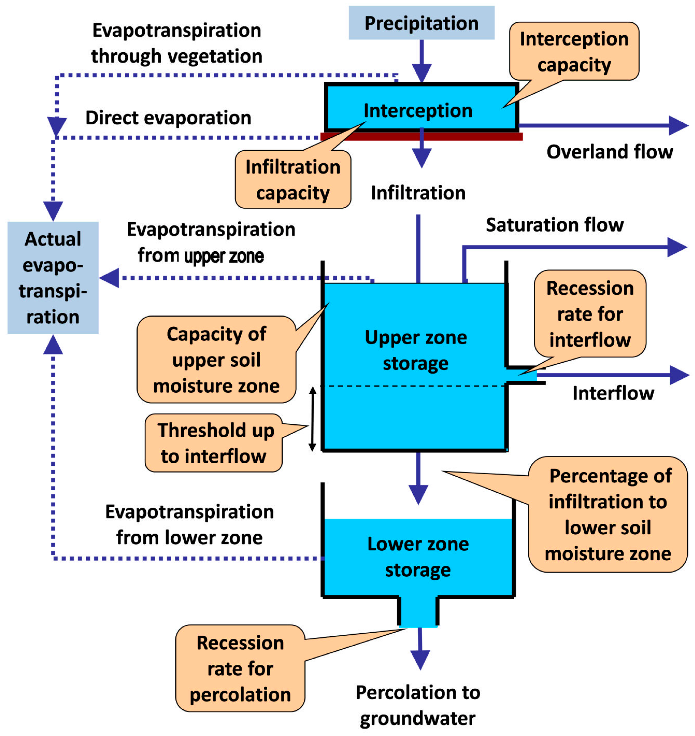
The model, in its general form, comprises seven parameters per HRU, one parameter per sub-basin, one parameter per river segment and two parameters per groundwater cell. In order to reduce the number of parameters of the groundwater module, for which it is often difficult to gather detailed spatial information (e.g., piezometric data), it is recommended to group cells with common hydraulic properties. For the estimation of the unknown parameters, an advanced calibration module is embedded that provides a set of statistical and empirical criteria for model fitting to multiple responses (e.g., river and spring discharge) and several options for the definition of the search space. These criteria include: (a) typical statistical metrics, such as efficiency or Nash–Sutcliffe index [98] and bias, aiming to ensure as close a fit as possible of the simulated flows against the observed ones; (b) penalties for flow intermittencies, which are easily observable information and very important from a water management perspective; and (c) trend penalties, to prohibit generating unrealistic flow or groundwater level patterns, based on the Mann–Kendall rank correlation test [99] (pp. 32–34). In the last version of HYDROGEIOS, a modified efficiency index has also been introduced to account for flow values above the observed mean, thus further forcing fitting to flood fluxes. According to the available information, the user may use multiple criteria aggregated in a weighted objective function. The function and the parameter bounds are inputs to a composite calibration problem, which is handled through an advanced global optimization technique, i.e., the evolutionary annealing-simplex algorithm [94,100,101].
References
- Beven, K.J. Changing Ideas in Hydrology—The Case of Physicallybased Models. J. Hydrol. 1989, 105, 157–172. [Google Scholar] [CrossRef]
- Boyle, D.P.; Gupta, H.V.; Sorooshian, S.; Koren, V.; Zhang, Z.; Smith, M. Towards Improved Streamflow Forecasts: The Value of Semidistributed Modeling. Water Resour. Res. 2001, 37, 2749–2759. [Google Scholar] [CrossRef]
- Ajami, N.K.; Gupta, H.; Wagener, T.; Sorooshian, S. Calibration of a Semi-Distributed Hydrologic Model for Streamflow Estimation along a River System. J. Hydrol. 2004, 298, 112–135. [Google Scholar] [CrossRef]
- Nalbantis, I.; Efstratiadis, A.; Rozos, E.; Kopsiafti, M.; Koutsoyiannis, D. Holistic versus Monomeric Strategies for Hydrological Modelling of Human-Modified Hydrosystems. Hydrol. Earth Syst. Sci. 2011, 15, 743–758. [Google Scholar] [CrossRef]
- Eckhardt, K.; Arnold, J.G. Automatic Calibration of a Distributed Catchment Model. J. Hydrol. 2001, 251, 103–109. [Google Scholar] [CrossRef]
- Fatichi, S.; Vivoni, E.R.; Ogden, F.L.; Ivanov, V.Y.; Mirus, B.; Gochis, D.; Downer, C.W.; Camporese, M.; Davison, J.H.; Ebel, B.; et al. An Overview of Current Applications, Challenges, and Future Trends in Distributed Process-Based Models in Hydrology. J. Hydrol. 2016, 537, 45–60. [Google Scholar] [CrossRef]
- Refsgaard, J.C. Parameterisation, Calibration and Validation of Distributed Hydrological Models. J. Hydrol. 1997, 198, 69–97. [Google Scholar] [CrossRef]
- Beven, K.J.; Binley, A.M. The Future of Distributed Models: Model Calibration and Uncertainty Prediction. Hydrol. Process. 1992, 6, 279–298. [Google Scholar] [CrossRef]
- Efstratiadis, A.; Nalbantis, I.; Koukouvinos, A.; Rozos, E.; Koutsoyiannis, D. HYDROGEIOS: A Semi-Distributed GIS-Based Hydrological Model for Modified River Basins. Hydrol. Earth Syst. Sci. 2008, 12, 989–1006. [Google Scholar] [CrossRef]
- Arnold, J.G.; Allen, P.M.; Bernhardt, G. A Comprehensive Surface-Groundwater Flow Model. J. Hydrol. 1993, 142, 47–69. [Google Scholar] [CrossRef]
- Neitsch, S.L.; Arnold, J.G.; Kiniry, J.R.; Williams, J.R. Soil and Water Assessment Tool Theoretical Documentation, Version 2005; Texas Water Resources Institute: Temple, TX, USA, 2005. [Google Scholar]
- Zhang, H.L.; Wang, Y.J.; Wang, Y.Q.; Li, D.X.; Wang, X.K. The Effect of Watershed Scale on HEC-HMS Calibrated Parameters: A Case Study in the Clear Creek Watershed in Iowa, US. Hydrol. Earth Syst. Sci. 2013, 17, 2735–2745. [Google Scholar] [CrossRef]
- Beven, K.J. Prophecy, Reality and Uncertainty in Distributed Hydrological Modelling. Adv. Water Resour. 1993, 16, 41–51. [Google Scholar] [CrossRef]
- Hromadka, T.V. San Bernardino County Hydrology Manual; Williamson and Schmid: Irvine, CA, USA, 1986. [Google Scholar]
- Dehotin, J.; Braud, I. Which Spatial Discretization for Distributed Hydrological Models? Proposition of a Methodology and Illustration for Medium to Large Scale Catchments. Hydrol. Earth Syst. Sci. 2008, 12, 769–796. [Google Scholar] [CrossRef]
- Cho, H.; Olivera, F. Effect of the Spatial Variability of Land Use, Soil Type, and Precipitation on Streamflows in Small Watersheds. J. Am. Water Resour. Assoc. 2009, 45, 673–686. [Google Scholar] [CrossRef]
- Han, J.-C.; Huang, G.-H.; Zhang, H.; Li, Z.; Li, Y.-P. Effects of Watershed Subdivision Level on Semi-Distributed Hydrological Simulations: Case Study of the SLURP Model Applied to the Xiangxi River Watershed, China. Hydrol. Sci. J. 2014, 59, 108–125. [Google Scholar] [CrossRef]
- Li, Z.; Li, L.; Huang, P.; Li, Q. Effect of Watershed Subdivision on Confluence Parameter. J. Hohai Univ. 2014, 42, 283–288. [Google Scholar]
- Savenije, H.H.G. HESS Opinions “Topography Driven Conceptual Modelling (FLEX-Topo)”. Hydrol. Earth Syst. Sci. 2010, 14, 2681–2692. [Google Scholar] [CrossRef]
- Rennό, C.D.; Nobre, A.D.; Cuartas, L.A.; Soares, J.V.; Hodnett, M.G.; Tomasella, J.; Waterloo, M.J. HAND, a New Terrain Descriptor Using SRTM-DEM: Mapping Terra-Firme Rainforest Environments in Amazonia. Remote Sens. Environ. 2008, 112, 3469–3481. [Google Scholar] [CrossRef]
- Donnelly, C.; Andersson, J.C.M.; Arheimer, B. Using Flow Signatures and Catchment Similarities to Evaluate the E-HYPE Multi-Basin Model across Europe. Hydrol. Sci. J. 2016, 61, 255–273. [Google Scholar] [CrossRef]
- Gharari, S.; Hrachowitz, M.; Fenicia, F.; Savenije, H.H.G. Hydrological Landscape Classification: Investigating the Performance of HAND Based Landscape Classifications in a Central European Meso-Scale Catchment. Hydrol. Earth Syst. Sci. 2011, 15, 3275–3291. [Google Scholar] [CrossRef]
- Bingner, R.L.; Garbrecht, J.; Arnold, J.G.; Srinivasan, R. Effect of Watershed Subdivision on Simulation Runoff and Fine Sediment Yield. Trans. Am. Soc. Agric. Eng. 1997, 40, 1329–1335. [Google Scholar] [CrossRef]
- Boyd, M.J.; Pilgrim, D.H.; Cordery, I. A Storage Routing Model Based on Catchment Geomorphology. J. Hydrol. 1979, 42, 209–230. [Google Scholar] [CrossRef]
- Goodrich, D.C.; Woolhiser, D.A.; Sorooshian, S. Model Complexity Required to Maintain Hydrologic Response. In Proceedings ASCE National Conference on Hydraulic Engineering; Abt, S.A., Gessler, J., Eds.; American Society of Civil Engineers (ASCE): Colorado Springs, CO, USA, 1988; pp. 431–463. [Google Scholar]
- Goodrich, D.C. An Overview of the USDA-ARS Climate Change and Hydrology Program and Analysis of Model Complexity as a Function of Basin Scale. In Proceedings of the Workshop on the Effects of Global Climate Change on Hydrology and Water Resources at Catchment Scale, Tsukuba, Japan, 3–6 February 1992; pp. 233–242. [Google Scholar]
- Norris, G.R. A Proccess for Interfacing a Hydrologic Model to a Geographic Information System. Mater’s Thesis, Oklahoma State University, Stillwater, OK, USA, 1992. [Google Scholar]
- Norris, G.R.; Haan, C.T. Impact of Subdivining Watersheds on Estimated Hydrographs. Am. Soc. Agric. Eng. 1993, 9, 443–445. [Google Scholar] [CrossRef]
- Zhang, Z.; Koren, V.; Smith, M.; Reed, S.; Wang, D. Use of Next Generation Weather Radar Data and Basin Disaggregation to Improve Continuous Hydrograph Simulations. J. Hydrol. Eng. 2004, 9, 103–115. [Google Scholar] [CrossRef]
- Arabi, M.; Govindaraju, R.S.; Hantush, M.M.; Engel, B.A. Role of Watershed Subdivision on Modeling the Effectiveness of Best Management Practices With Swat 1. J. Am. Water Resour. Assoc. 2006, 45268, 513–528. [Google Scholar] [CrossRef]
- Cho, J.; Lowrance, R.R.; Bosch, D.D.; Strickland, T.C.; Her, Y.; Vellidis, G. Effect of Watershed Subdivision and Filter Width on Swat Simulation of a Coastal Plain watershed1. J. Am. Water Resour. Assoc. 2010, 46, 586–602. [Google Scholar] [CrossRef]
- FitzHugh, T.W.; Mackay, D.S. Impacts of Input Parameter Spatial Aggregation on an Agricultural Nonpoint Source Pollution Model. J. Hydrol. 2000, 236, 35–53. [Google Scholar] [CrossRef]
- Kalin, L.; Govindaraju, R.S.; Hantush, M.M. Effect of Geomorphologic Resolution on Modeling of Runoff Hydrograph and Sedimentograph over Small Watersheds. J. Hydrol. 2003, 276, 89–111. [Google Scholar] [CrossRef]
- Kumar, S.; Merwade, V. Impact of Watershed Subdivision and Soil Data Resolution on Swat Model Calibration and Parameter Uncertainty. J. Am. Water Resour. Assoc. 2009, 45, 1179–1196. [Google Scholar] [CrossRef]
- Muleta, M.K.; Nicklow, J.W.; Bekele, E.G. Sensitivity of a Distributed Watershed Simulation Model to Spatial Scale. J. Hydrol. Eng. 2007, 12, 163–172. [Google Scholar] [CrossRef]
- Thieken, A.H.; Lücke, A.; Diekkrüger, B.; Richter, O. Scaling Input Data by GIS for Hydrological Modelling. Hydrol. Process. 1999, 13, 611–630. [Google Scholar] [CrossRef]
- Nour, M.H.; Smith, D.W.; El-Din, M.G.; Prepas, E.E. Effect of Watershed Subdivision on Water-Phase Phosphorus Modelling: An Artificial Neural Network Modelling Application. J. Environ. Eng. Sci. 2008, 7, 95–108. [Google Scholar] [CrossRef]
- Kite, G.W. Manual for the SLURP Hydrological Model; The National Health Research Institutes (NHRI): Saskatoon, SK, Canada, 1997. [Google Scholar]
- Bathurst, J.C. Sensitivity Analysis of the Systeme Hydrologique Europeen for an Upland Catchment. J. Hydrol. 1986, 87, 103–123. [Google Scholar] [CrossRef]
- Bruneau, P.; Gascuel-Odoux, C.; Robin, P.; Merot, P.; Beven, K. Sensitivity to Space and Time Resolution of a Hydrological Model Using Digital Elevation Data. Hydrol. Process. 1995, 9, 69–81. [Google Scholar] [CrossRef]
- Manguerra, H.B.; Engel, B.A. Hydrologic Parameterization of Watersheds for Runoff Prediction Using SWAT. J. Am. Water Resour. Assoc. 1998, 34, 1149–1162. [Google Scholar] [CrossRef]
- Molnár, D.K.; Julien, P.Y. Grid-Size Effects on Surface Runoff Modeling. J. Hydrol. Eng. 2000, 5, 8–16. [Google Scholar] [CrossRef]
- Tao, T.; Kouwen, N. Remote Sensing and Fully Distributed Modelling for Flood Forecasting. J. Water Resour. Plan. Manag. 1989, 115, 809–823. [Google Scholar] [CrossRef]
- Zhang, W.; Montgomery, D.R. Digital Elevation Model Grid Size, Landscape Representation, and Hydrologic Simulations. Water Resour. Res. 1994, 30, 1019–1028. [Google Scholar] [CrossRef]
- Wood, E.F.; Sivapalan, M.; Beven, K.; Band, L. Effects of Spatial Variability and Scale with Implications to Hydrologic Modeling. J. Hydrol. 1988, 102, 29–47. [Google Scholar] [CrossRef]
- Sasowsky, K.C.; Gardner, T.W. Watershed Configuration and Geographic Information System Parameterization for SPUR Model Hydrologic Simulations. J. Am. Water Resour. Assoc. 1991, 27, 7–18. [Google Scholar] [CrossRef]
- Reggiani, P.; Sivapalan, M.; Hassanizadeh, S.M. A Unifying Framework for Watershed Thermodynamics: Balance Equations for Mass, Momentum, Energy and Entropy, and the Second Law of Thermodynamics. Adv. Water Resour. 1998, 22, 367–398. [Google Scholar] [CrossRef]
- Reggiani, P.; Hassanizadeh, S.M.; Sivapalan, M.; Gray, W.G. A Unifying Framework for Watershed Thermodynamics: Constitutive Relationships. Adv. Water Resour. 1999, 23, 15–39. [Google Scholar] [CrossRef]
- Reggiani, P.; Sivapalan, M.; Hassanizadeh, S. Conservation Equations Governing Hillslope Responses: Exploring the Physical Basis of Water Balance. Water Resour. Res. 2000, 36, 1845–1863. [Google Scholar] [CrossRef]
- Reggiani, P.; Rientjes, T.H.M. Flux Parameterization in the Representative Elementary Watershed Approach: Application to a Natural Basin. Water Resour. Res. 2005, 41, 1–18. [Google Scholar] [CrossRef]
- Daniel, E.B. Watershed Modeling and Its Applications: A State-of-the-Art Review. Open Hydrol. J. 2011, 5, 26–50. [Google Scholar] [CrossRef]
- Leavesley, G.H.; Lichty, R.W.; Troutman, B.M.; Saindon, L.G. Precipitation-Runoff Modeling System: User’s Manual; United States Geological Survey (USGS): Denver, CO, USA, 1983.
- Flügel, W.-A. Delineating Hydrological Response Units by Geographical Information System Analyses for Regional Hydrological Modelling Using PRMS/MMS in the Drainage Basin of the River Brosl, Germany. Hydrol. Process. 1995, 9, 423–436. [Google Scholar] [CrossRef]
- Leavesley, G.H.; Stannard, L.G. The Precipitation-Runoff Modeling System-PRMS. In Computer Models of Watershed Hydrology; Singh, V.P., Ed.; Water Resources Publication: Highlands Ranch, CO, USA, 1995; p. 1144. [Google Scholar]
- Flügel, W.-A. Combining GIS with Regional Hydrological Modelling Using Hydrological Response Units (HRUs): An Application from Germany. Math. Comput. Simul. 1997, 43, 297–304. [Google Scholar] [CrossRef]
- Bongartz, K. Applying Different Spatial Distribution and Modelling Concepts in Three Nested Mesoscale Catchments of Germany. Phys. Chem. Earth 2003, 28, 1343–1349. [Google Scholar] [CrossRef]
- Srinivasan, R.; Muttiah, R.S.; Dyke, P.T.; Walker, C.; Arnold, J. Hydrologic Unit Model for the United States (HUMUS); Texas Agricultural Experiment Station: Temple, TX, USA, 2000. [Google Scholar]
- Neitsch, S.L.; Arnold, J.G.; Kiniry, J.R.; Williams, J.R.; King, K.W. Soil and Water Assessment Tool Theoretical Documentation, Version 2000; Texas Water Resources Institute: Temple, TX, USA, 2002. [Google Scholar]
- Gitau, M.W. A Quantitative Assessment of BMP Effectiveness for Phosphorus Pollution Control: The Town Brook Watershed; The Pennsylvannia State University: State College, PA, USA, 2003. [Google Scholar]
- Gassman, P.W.; Reyes, M.R.; Green, C.H.; Arnold, J.G. The Soil and Water Assessment Tool: Historical Development, Applications, and Future Research Directions. Trans. Asabe 2007, 50, 1211–1250. [Google Scholar] [CrossRef]
- Gassman, P.W. A Simulation Assessment of the Boone River Watershed: Baseline Calibration/Validation Results and Issues, and Future Needs. Ph.D. Thesis, Iowa State University, Ameas, IA, USA, 2008. [Google Scholar]
- The National Regulator for Compulsory Specifications (NRCS). SCS National Engineering Handbook, Section 4; NRCS: Washington, DC, USA, 1972. [Google Scholar]
- The National Regulator for Compulsory Specifications (NRCS). National Engineering Handbook: Part 630—Hydrology; The National Regulator for Compulsory Specifications (NRCS): Washington, DC, USA, 2004. [Google Scholar]
- Soulis, K.X.; Valiantzas, J.D. SCS-CN Parameter Determination Using Rainfall-Runoff Data in Heterogeneous Watersheds—The Two-CN System Approach. Hydrol. Earth Syst. Sci. 2012, 16, 1001–1015. [Google Scholar] [CrossRef] [Green Version]
- Banasik, K.; Rutkowska, A.; Kohnová, S. Retention and Curve Number Variability in a Small Agricultural Catchment: The Probabilistic Approach. Water 2014, 6, 1118–1133. [Google Scholar] [CrossRef]
- Montgomery, D.R.; Dietrich, W.E. Runoff Generation in a Steep, Soil-Mantled Landscape. Water Resour. Manag. 2002, 38, 1168. [Google Scholar] [CrossRef]
- Huang, M.; Gallichand, J.; Wang, Z.; Goulet, M. A Modification to the Soil Conservation Service Curve Number Method for Steep Slopes in the Loess Plateau of China. Hydrol. Process. 2006, 20, 579–589. [Google Scholar] [CrossRef]
- Xu, Y.; Fu, B.; Gao, G.; He, C. Watershed Discretization Based on Multiple Factors and Its Application in the Chinese Loess Plateau. Hydrol. Earth Syst. Sci. 2011, 8, 9063–9087. [Google Scholar] [CrossRef]
- Deshmukh, D.S.; Chaube, U.C.; Hailu, A.E.; Gudeta, D.A.; Kassa, M.T. Estimation and Comparison of Curve Numbers Based on Dynamic Land Use Land Cover Change, Observed Rainfall-Runoff Data and Land Slope. J. Hydrol. 2013, 492, 89–101. [Google Scholar] [CrossRef]
- Verma, S.; Verma, R.K.; Mishra, S.K.; Singh, A.; Jayaraj, G.K. A Revisit of NRCS-CN Inspired Models Coupled with RS and GIS for Runoff Estimation. Hydrol. Sci. J. 2017, 62, 1891–1930. [Google Scholar] [CrossRef]
- Merheb, M.; Moussa, R.; Abdallah, C.; Colin, F.; Perrin, C.; Baghdadi, N. Hydrological Response Characteristics of Mediterranean Catchments at Different Time Scales: A Meta-Analysis. Hydrol. Sci. J. 2016, 61, 2520–2539. [Google Scholar] [CrossRef]
- Efstratiadis, A.; Koussis, A.D.; Koutsoyiannis, D.; Mamassis, N. Flood Design Recipes vs. Reality: Can Predictions for Ungauged Basins Be Trusted? Nat. Hazards Earth Syst. Sci. 2014, 14, 1417–1428. [Google Scholar] [CrossRef]
- Efstratiadis, A.; Koukouvinos, A.; Michaelidi, E.; Galiouna, E.; Tzouka, K.; Koussis, A.D.; Mamassis, N.; Koutsoyiannis, D. Description of Regional Approaches for the Estimation of Characteristic Hydrological Quantities, DEUCALION—Assessment of Flood Flows in Greece under Conditions of Hydroclimatic Variability: Development of Physically-Established Conceptual-Probabilistic; Department of Water Resources and Environmental Engineering—National Technical University of Athens, National Observatory of Athens: Athens, Greece, 2014. [Google Scholar]
- Kowalik, T.; Walega, A. Estimation of CN Parameter for Small Agricultural Watersheds Using Asymptotic Functions. Water 2015, 7, 939–955. [Google Scholar] [CrossRef]
- Efstratiadis, A.; Koutsoyiannis, D. One Decade of Multiobjective Calibration Approaches in Hydrological Modelling: A Review. Hydrol. Sci. J. 2010, 55, 58–78. [Google Scholar] [CrossRef]
- Jakeman, A.J.; Hornberger, G.M. How Much Complexity Is Warranted in a Rainfall-Runoff Model? Water Resour. Res. 1993, 29, 2637–2649. [Google Scholar] [CrossRef]
- Fenicia, F.; Kavetski, D.; Savenije, H.H.G.; Clark, M.P.; Schoups, G.; Pfister, L.; Freer, J. Catchment Properties, Function, and Conceptual Model Representation: Is There a Correspondence? Hydrol. Process. 2014, 28, 2451–2467. [Google Scholar] [CrossRef]
- Wheater, H.S.; Bishop, K.H.; Beck, M.B. He Identification of Conceptual Hydrological Models for Surface Water Acidification. Hydrol. Process. 1986, 1, 89–109. [Google Scholar] [CrossRef]
- Wagener, T.; Boyle, D.P.; Lees, M.J.; Wheater, H.S.; Gupta, H.V.; Sorooshian, S. A Framework for Development and Application of Hydrological Models. Hydrol. Earth Syst. Sci. 2001, 5, 13–26. [Google Scholar] [CrossRef]
- Fenicia, F.; Kavetsi, D.; Savenije, H.H.G.; Pfister, L. From Spatially Variable Streamflow Todistributed Hydrological Models: Analysis of Key Modeling Decisions. Water Resour. Res. 2016, 52, 1–36. [Google Scholar] [CrossRef]
- Pollacco, J.A.P.; Mohanty, B.P.; Efstratiadis, A. Weighted Objective Function Selector Algorithm for Parameter Estimation of SVAT Models with Remote Sensing Data. Water Resour. Res. 2013, 49, 6959–6978. [Google Scholar] [CrossRef]
- Silvestro, F.; Gabellani, S.; Rudari, R.; Delogu, F.; Laiolo, P.; Boni, G. Uncertainty Reduction and Parameter Estimation of a Distributed Hydrological Model with Ground and Remote-Sensing Data. Hydrol. Earth Syst. Sci. 2015, 19, 1727–1751. [Google Scholar] [CrossRef]
- Efstratiadis, A.; Koukouvinos, A.; Dimitriadis, P.; Rozos, E.; Koussis, A.D. Theoretical Documentation of Hydrological-Hydraulic Simulation Model, DEUCALION—Assessment of Flood Flows in Greece under Conditions of Hydroclimatic Variability: Development of Physically-Established Conceptual-Probabilistic Framework and Computational; Department of Water Resources and Environmental Engineering—National Technical University of Athens, National Observatory of Athens: Athens, Greece, 2014. [Google Scholar]
- Koutsoyiannis, D.; Andreadakis, A.; Mavrodmou, R.; Christofides, A.; Mamassis, N.; Efstratiadis, A.; Koukouvinos, A.; Karavokiros, G.; Kozanis, S.; Mamais, D.; et al. National Programme for the Management and Protection of Water Resources; Department of Water Resources and Environmental Engineering—National Technical University of Athens: Athens, Greece, 2008. [Google Scholar]
- Efstratiadis, A.; Koussis, A.D.; Lykoudis, S.; Koukouvinos, A.; Christofides, A.; Karavokiros, G.; Kappos, N.; Mamassis, N.; Koutsoyiannis, D. Hydrometeorological Network for Flood Monitoring and Modeling. In Proceedings of First International Conference on Remote Sensing and Geoinformation of Environment; (SPIE) Society of Photo-Optical Instrumentation Engineers: Paphos, Cyprus, 2013; Volume 8795. [Google Scholar]
- Tegos, A.; Efstratiadis, A.; Koutsoyiannis, D. A Parametric Model for Potential Evapotranspiration Estimation Based on a Simplified Formulation of the Penman-Monteith Equation. In Evapotranspiration—An Overview; Alexandris, S.G., Ed.; InTech: Hongkong, China, 2013; p. 24. [Google Scholar]
- Tegos, A.; Malamos, N.; Efstratiadis, A.; Tsoukalas, I.; Karanasios, A.; Koutsoyiannis, D. Parametric Modelling of Potential Evapotranspiration: A Global Survey. Water 2017, 9, 795. [Google Scholar] [CrossRef]
- Freer, J.; Beven, K.J.; Ambroise, B. Bayesian Estimation of Uncertainty in Runoff Prediction and the Value of Data: An Application of the GLUE Approach. Water Resour. Manag. 1996, 32, 2161–2173. [Google Scholar] [CrossRef]
- Moriasi, D.N.; Arnold, J.G.; Van Liew, M.W.; Bingner, R.L.; Harmel, R.D.; Veith, T.L. Model Evaluation Guidelines for Systematic Quantification of Accuracy in Watershed Simulations. Trans. Am. Soc. Agric. Biol. Eng. 2007, 50, 885–900. [Google Scholar]
- Winchell, M.; Srinivasan, R.; Di Luzio, M.; Arnold, J.G. ArcSwat Interface for SWAT 2012: Users Guide; Blackland Research Centre, Texas Agrivcultural Experiment Station: Temple, TX, USA, 2013. [Google Scholar]
- Boyle, D.P.; Gupta, H.V.; Sorooshian, S. Toward Improved Calibration of Hydrologic Models: Combining the Strengths of Manual and Automatic Methods. Water Resour. Res. 2000, 36, 3663–3674. [Google Scholar] [CrossRef]
- Mazi, K.; Koussis, A.D.; Restrepo, P.J.; Koutsoyiannis, D. A Groundwater-Based, Objective-Heuristic Parameter Optimisation Method for the PRMS Model: The Akrotiri Basin, Cyprus Application. J. Hydrol. 2004, 290, 243–258. [Google Scholar] [CrossRef]
- Mazi, K.; Koussis, A.D.; Restrepo, P.J.; Koutsoyiannis, D. Erratum: A Groundwater-Based, Objective-Heuristic Parameter Optimisation Method for the PRMS Model: The Akrotiri Basin, Cyprus Application. J. Hydrol. 2004, 299, 160–161. [Google Scholar] [CrossRef]
- Rozos, E.; Efstratiadis, A.; Nalbantis, I.; Koutsoyiannis, D. Calibration of a Semi-Distributed Model for Conjunctive Simu-Lation of Surface and Groundwater Flow. Hydrol. Sci. J. 2004, 49, 819–842. [Google Scholar] [CrossRef]
- Rozos, E.; Koutsoyiannis, D. A Multicell Karstic Aquifer Model with Alternative Flow Equations. J. Hydrol. 2006, 325, 340–355. [Google Scholar] [CrossRef]
- Koussis, A.D. Assessment and Review of the Hydraulics of Storage Flood Routing 70 Years after the Presentation of the Muskingum Method. Hydrol. Sci. J. 2009, 54, 43–61. [Google Scholar] [CrossRef]
- Koussis, A.D. Reply to the Discussion of “Assessment and Review of the Hydraulics of Storage Flood Routing 70 Years after the Presentation of the Muskingum Method” by M. Perumal. Hydrol. Sci. J. 2010, 55, 1431–1441. [Google Scholar] [CrossRef]
- Nash, J.E.; Sutcliffe, J.V. River Flow Forecasting through Conceptual Models Part I—A Discussion of Principles. J. Hydrol. 1970, 10, 282–290. [Google Scholar] [CrossRef]
- Kottegoda, N.T. Stochastic Water Resources Technology; McMillan Press: Hong Kong, China, 1980. [Google Scholar]
- Efstratiadis, A.; Koutsoyiannis, D. An Evolutionary Annealing-Simplex Algorithm for Global Optimisation of Water Resource Systems. In Proceedings of the Fifth International Conference on Hydroinformatics; International Water Association: Cardiff, UK, 2002; pp. 1423–1428. [Google Scholar]
- Tsoukalas, I.; Kossieris, P.; Efstratiadis, A.; Makropoulos, C. Surrogate-Enhanced Evolutionary Annealing Simplex Algorithm for Effective and Efficient Optimization of Water Resources Problems on a Budget. Environ. Model. Softw. 2016, 77, 122–142. [Google Scholar] [CrossRef]
Figure 1.
(a) Layers of geographic information for permeability classes (), vegetation density classes () and drainage capacity classes (); (b) layer overlay; (c) CN parameter map.
Figure 1.
(a) Layers of geographic information for permeability classes (), vegetation density classes () and drainage capacity classes (); (b) layer overlay; (c) CN parameter map.
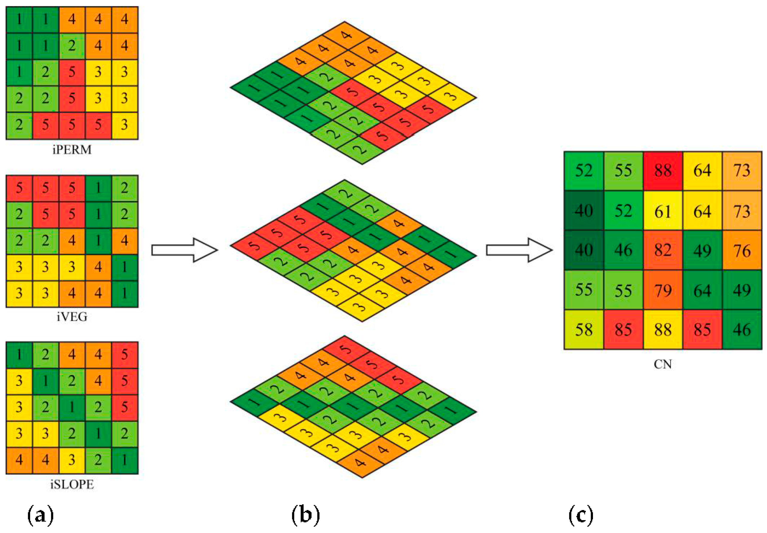
Figure 2.
Scatter plot of reference CN values and average flood runoff coefficients.
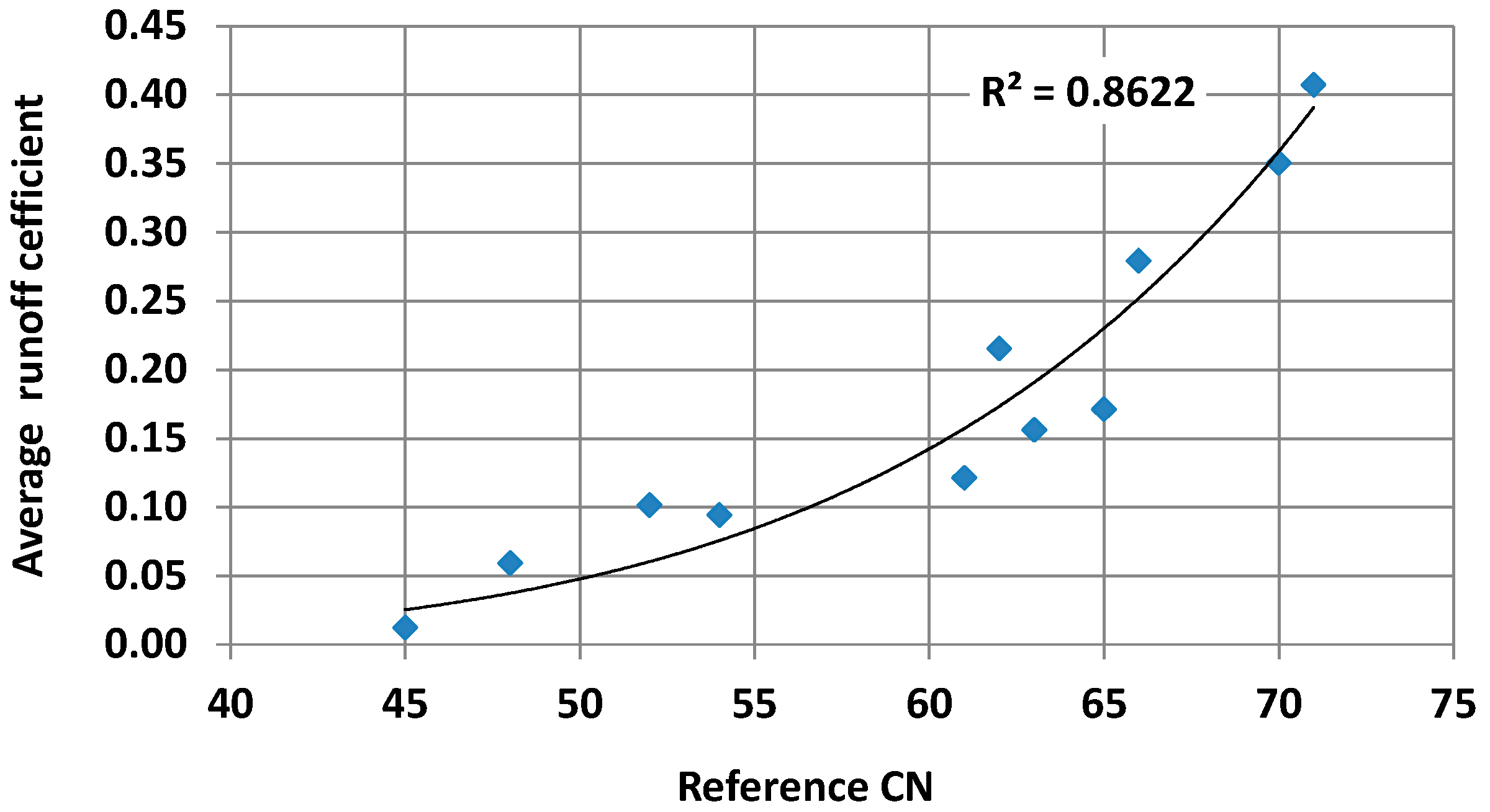
Figure 3.
HRU delineation based on the CN map: (a) CN parameter classes and (b) configuration of two HRUs, using CN = 63 as the threshold to determine the associated CN classes.
Figure 3.
HRU delineation based on the CN map: (a) CN parameter classes and (b) configuration of two HRUs, using CN = 63 as the threshold to determine the associated CN classes.

Figure 4.
Digital map of Nedontas River Basin, also showing monitoring stations (meteorological and hydrometric) and the main modelling components (junctions, sub-basins, river segments).
Figure 4.
Digital map of Nedontas River Basin, also showing monitoring stations (meteorological and hydrometric) and the main modelling components (junctions, sub-basins, river segments).
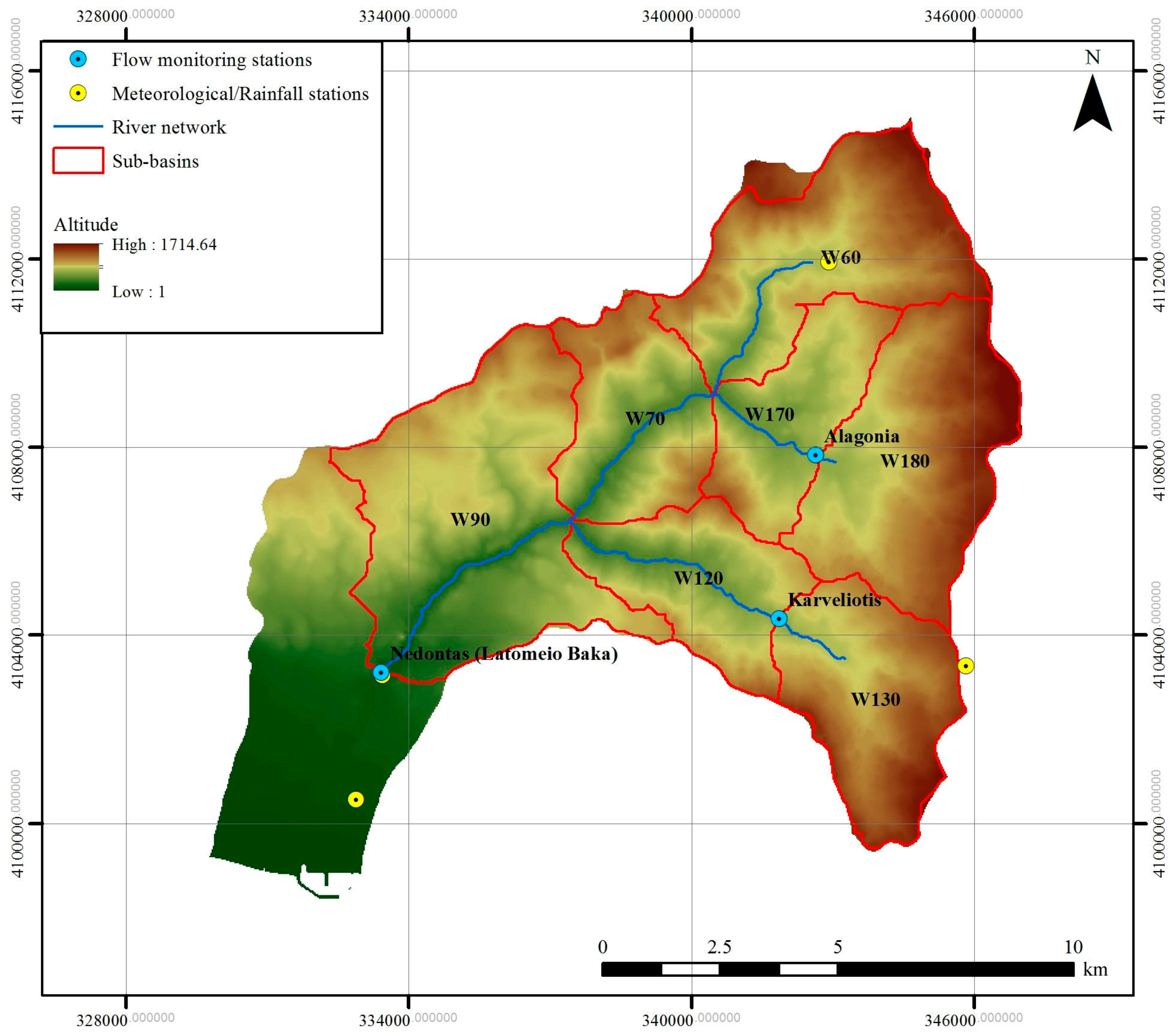
Figure 5.
(a) Water permeability classes; (b) land cover classes; (c) terrain slope (%) classes; (d) CN parameter map of the initial Nedontas River Basin map of 18 CN classes.
Figure 5.
(a) Water permeability classes; (b) land cover classes; (c) terrain slope (%) classes; (d) CN parameter map of the initial Nedontas River Basin map of 18 CN classes.


Figure 6.
HRU delineation based on (a) two, (b) three CN, (c) four and (d) five CN classes.

Figure 7.
HRU delineation of Nedontas River Basin: (a) SWAT GIS overlay and threshold definition method, 31 HRUs; (b) HYDROGEIOS union of layers method, four HRUs.
Figure 7.
HRU delineation of Nedontas River Basin: (a) SWAT GIS overlay and threshold definition method, 31 HRUs; (b) HYDROGEIOS union of layers method, four HRUs.
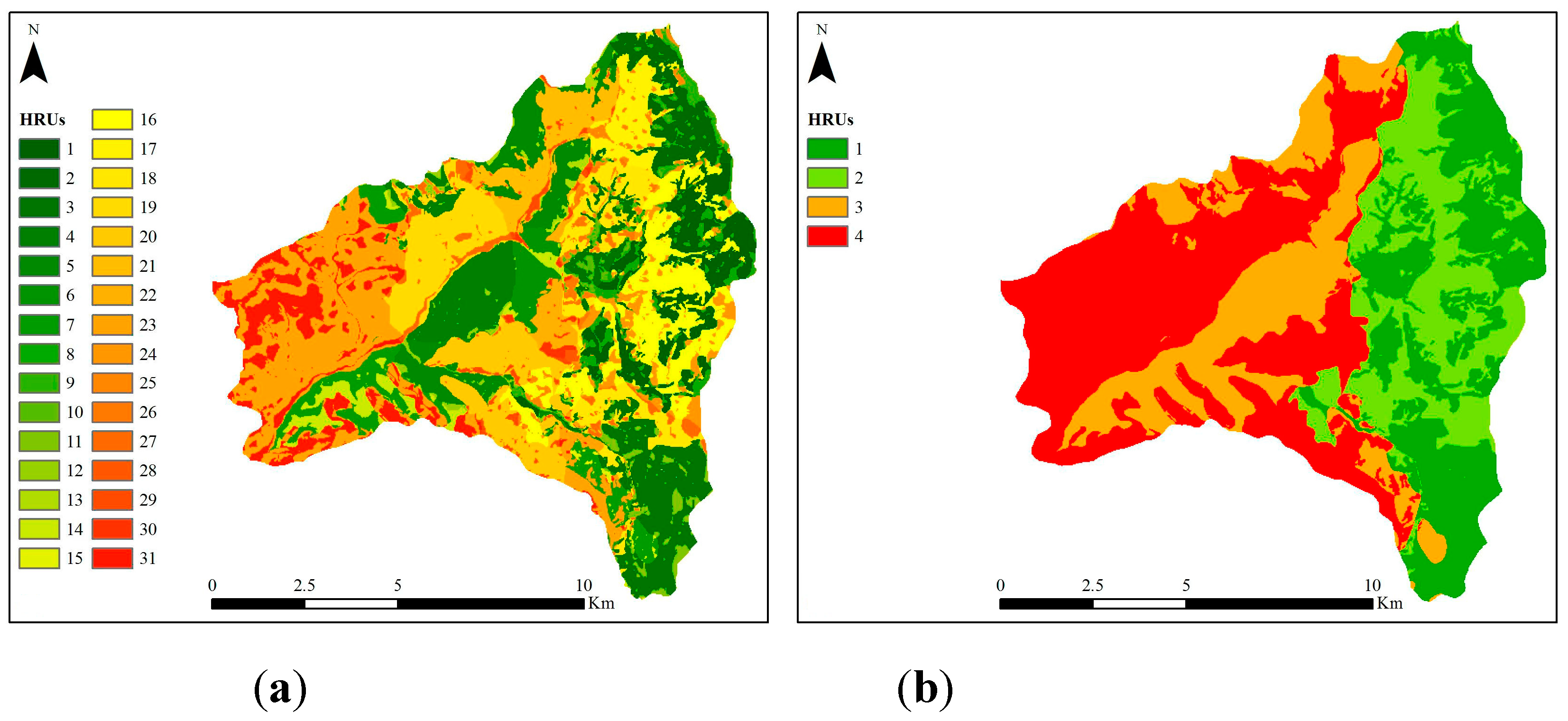
Figure 8.
Computed vs. observed discharge series at the basin outlet (Latomeio Baka) for HRU delineation with: (a) unique combination; (b) union of layers; (c) CN approach.
Figure 8.
Computed vs. observed discharge series at the basin outlet (Latomeio Baka) for HRU delineation with: (a) unique combination; (b) union of layers; (c) CN approach.
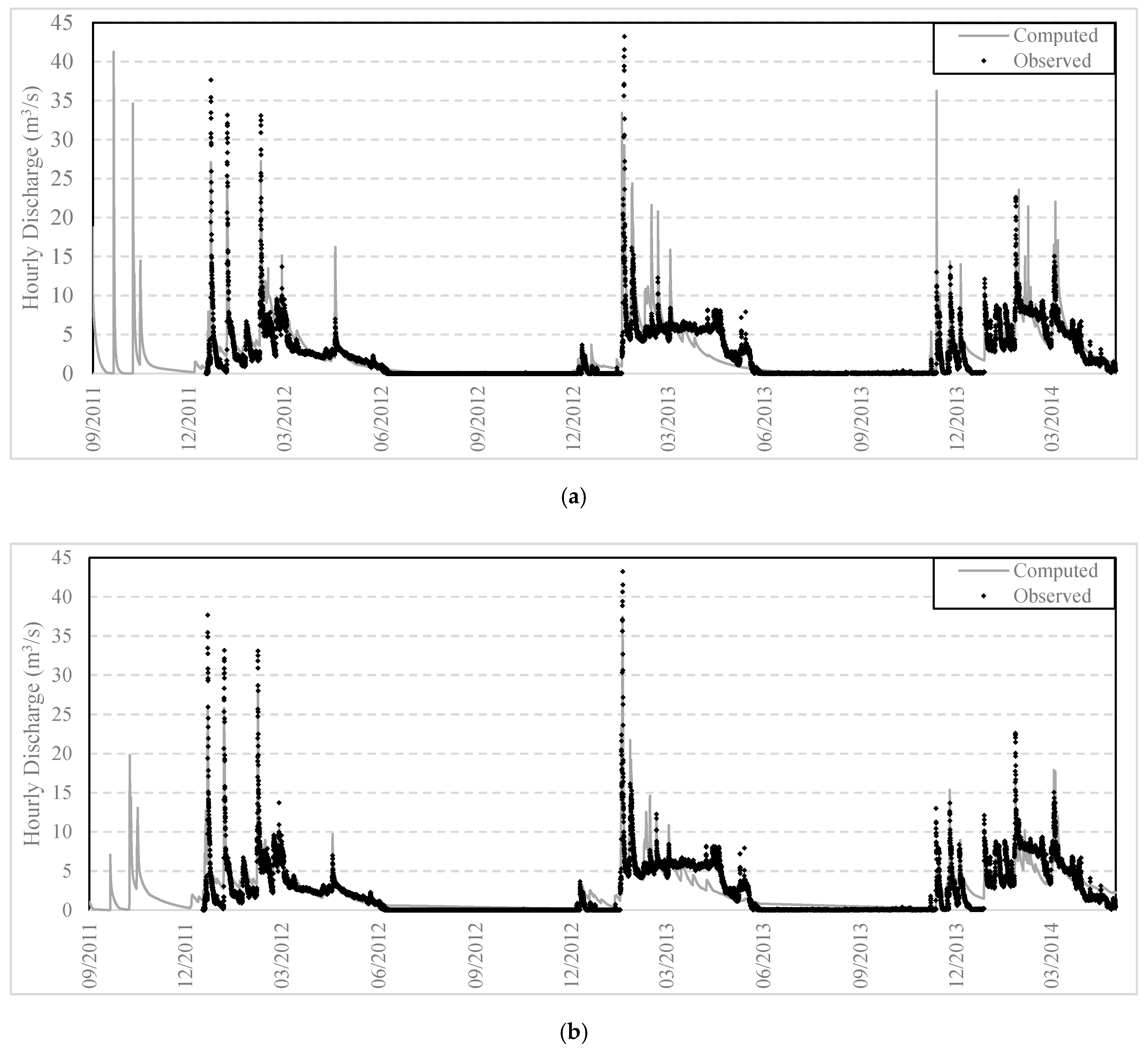
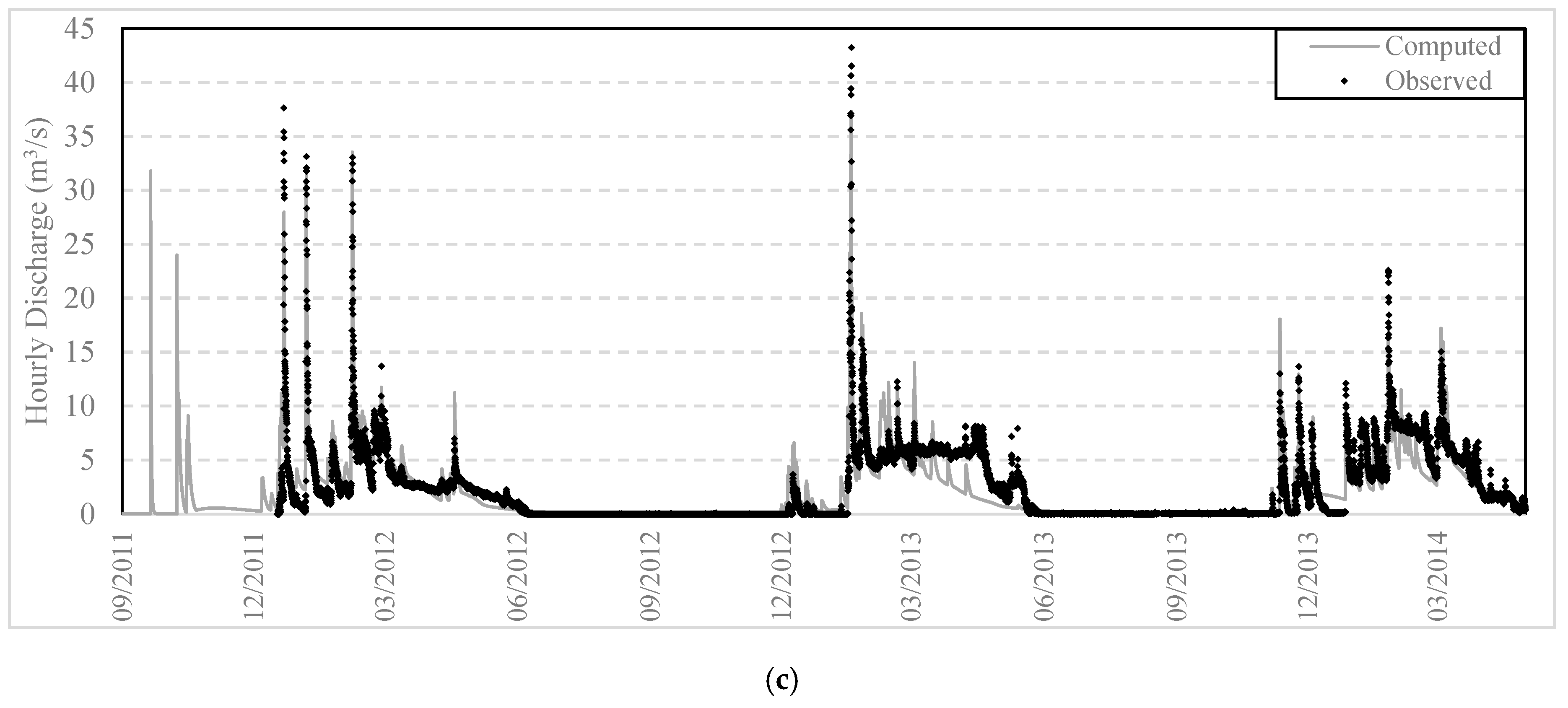
Figure 9.
Computed vs. observed discharge series at Karveliotis monitoring station for HRU delineation with: (a) unique combination; (b) union of layers; (c) CN approach.
Figure 9.
Computed vs. observed discharge series at Karveliotis monitoring station for HRU delineation with: (a) unique combination; (b) union of layers; (c) CN approach.
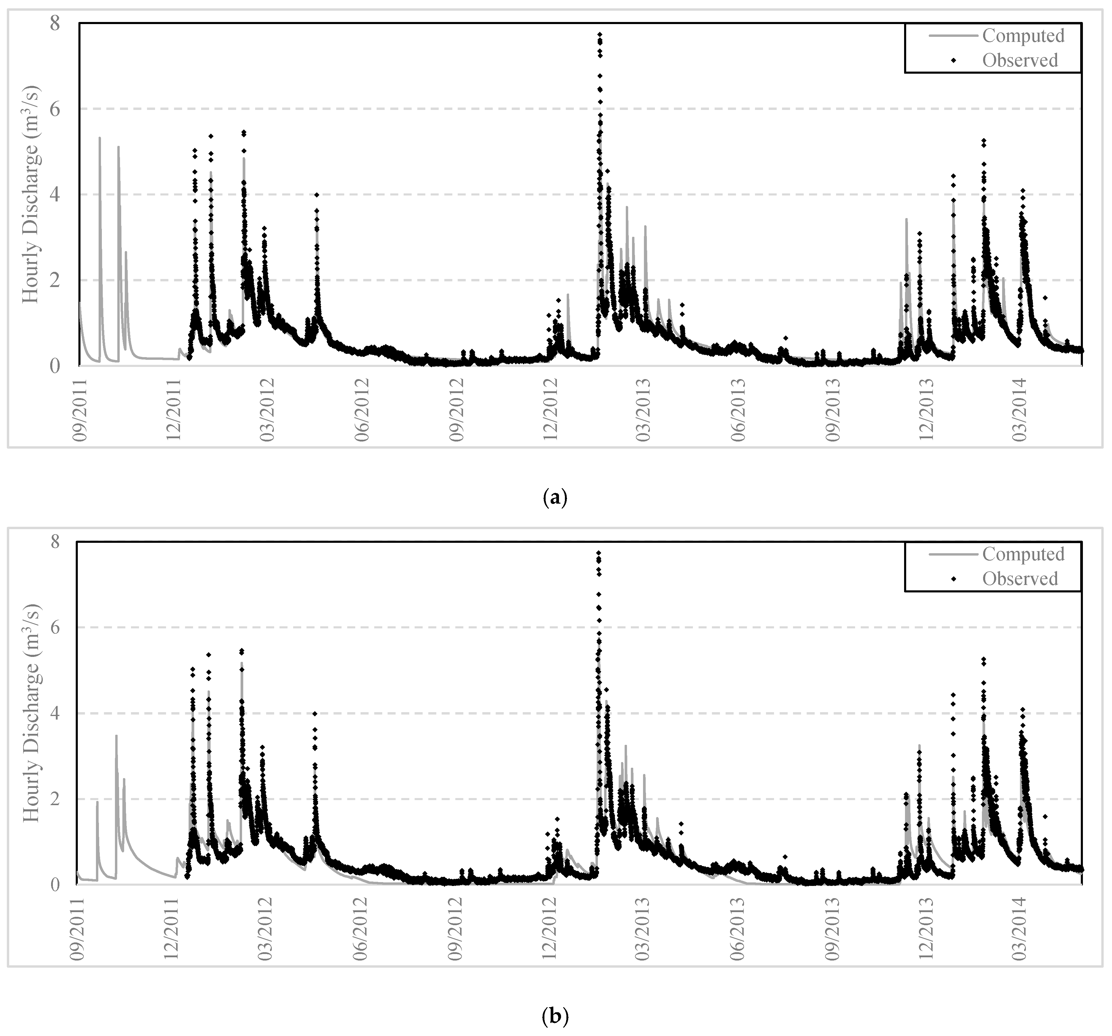

Figure 10.
Computed vs. observed discharge series at Alagonia monitoring station for HRU delineation with: (a) unique combination; (b) union of layers; (c) CN approach.
Figure 10.
Computed vs. observed discharge series at Alagonia monitoring station for HRU delineation with: (a) unique combination; (b) union of layers; (c) CN approach.
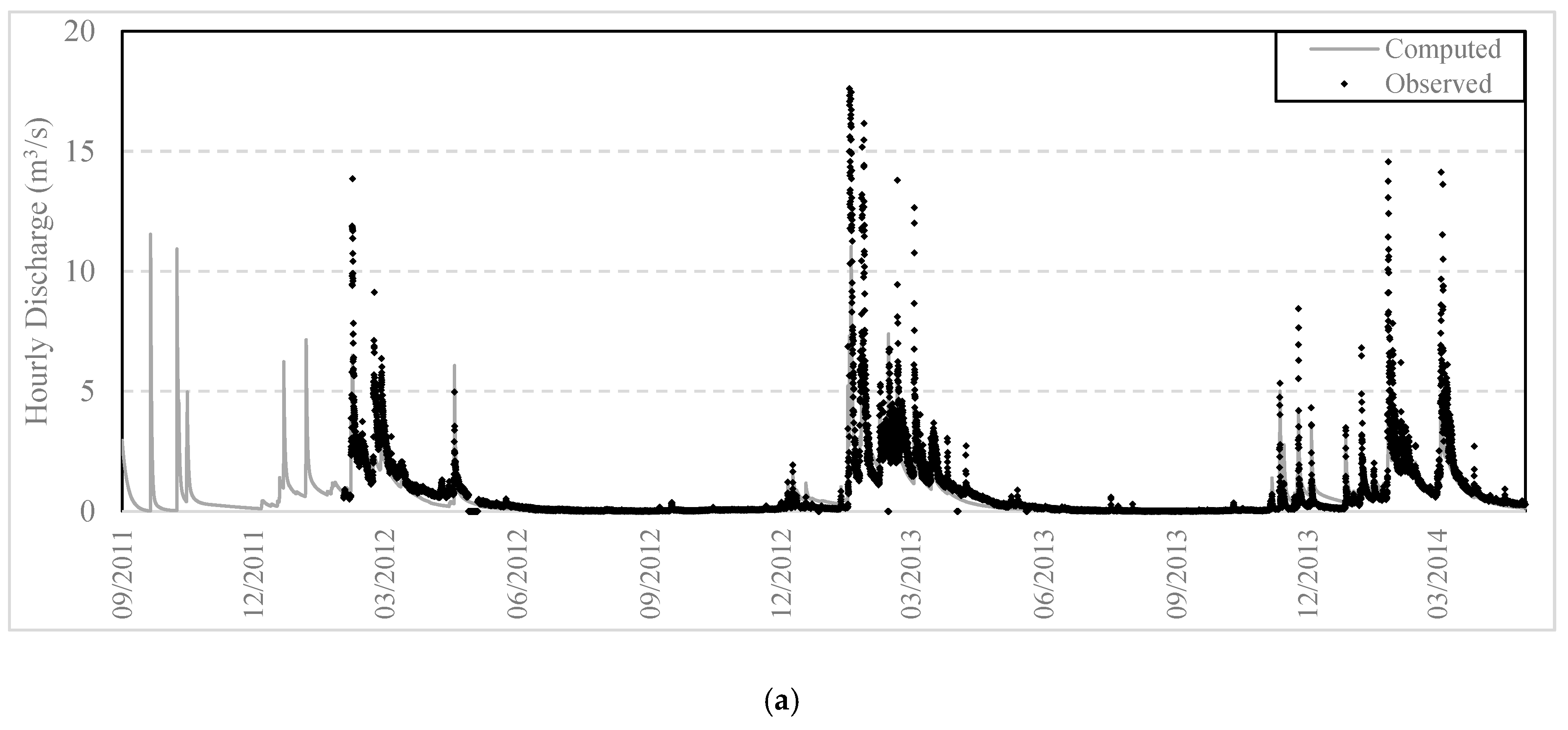


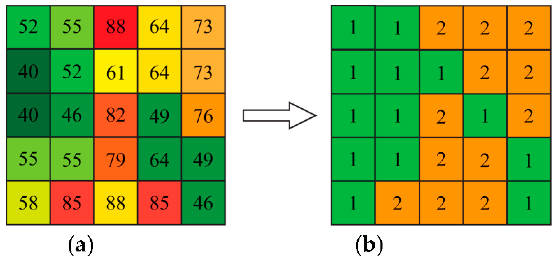
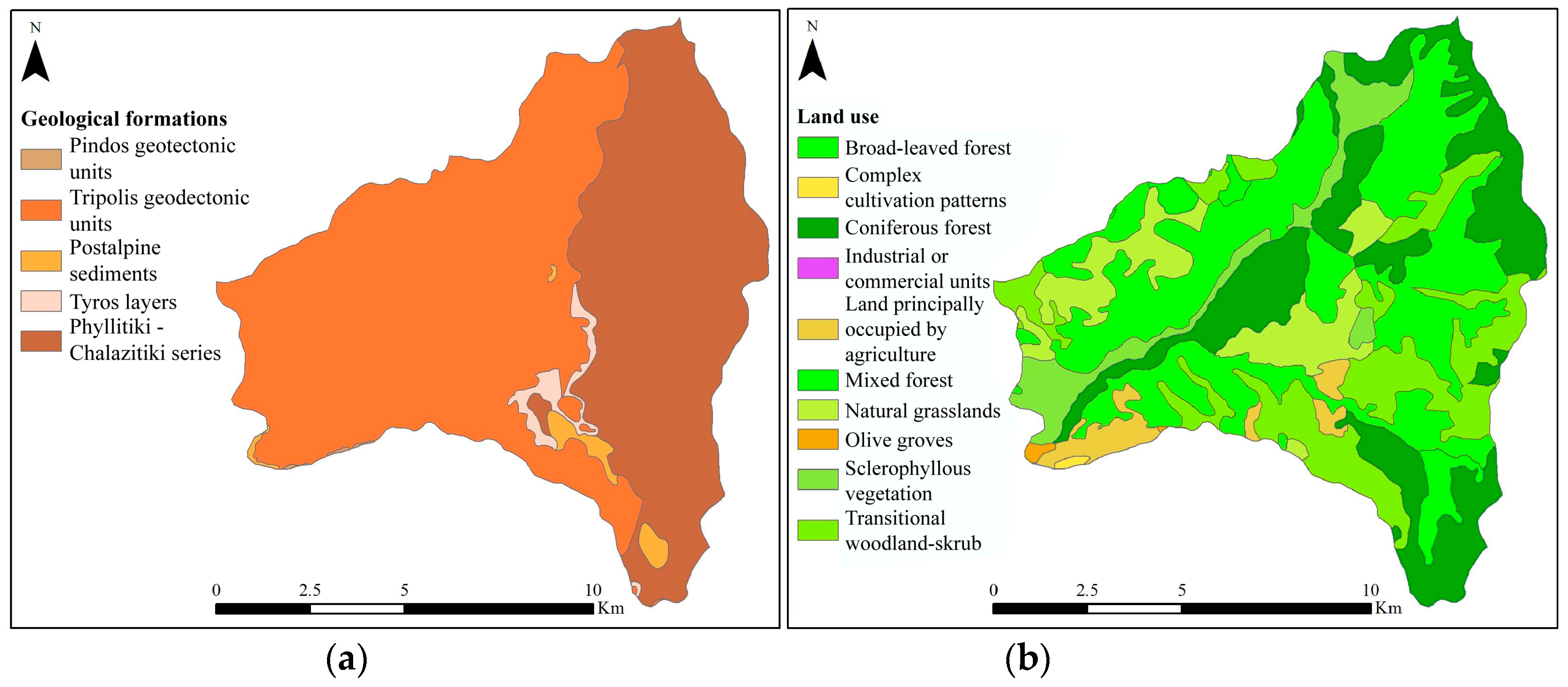
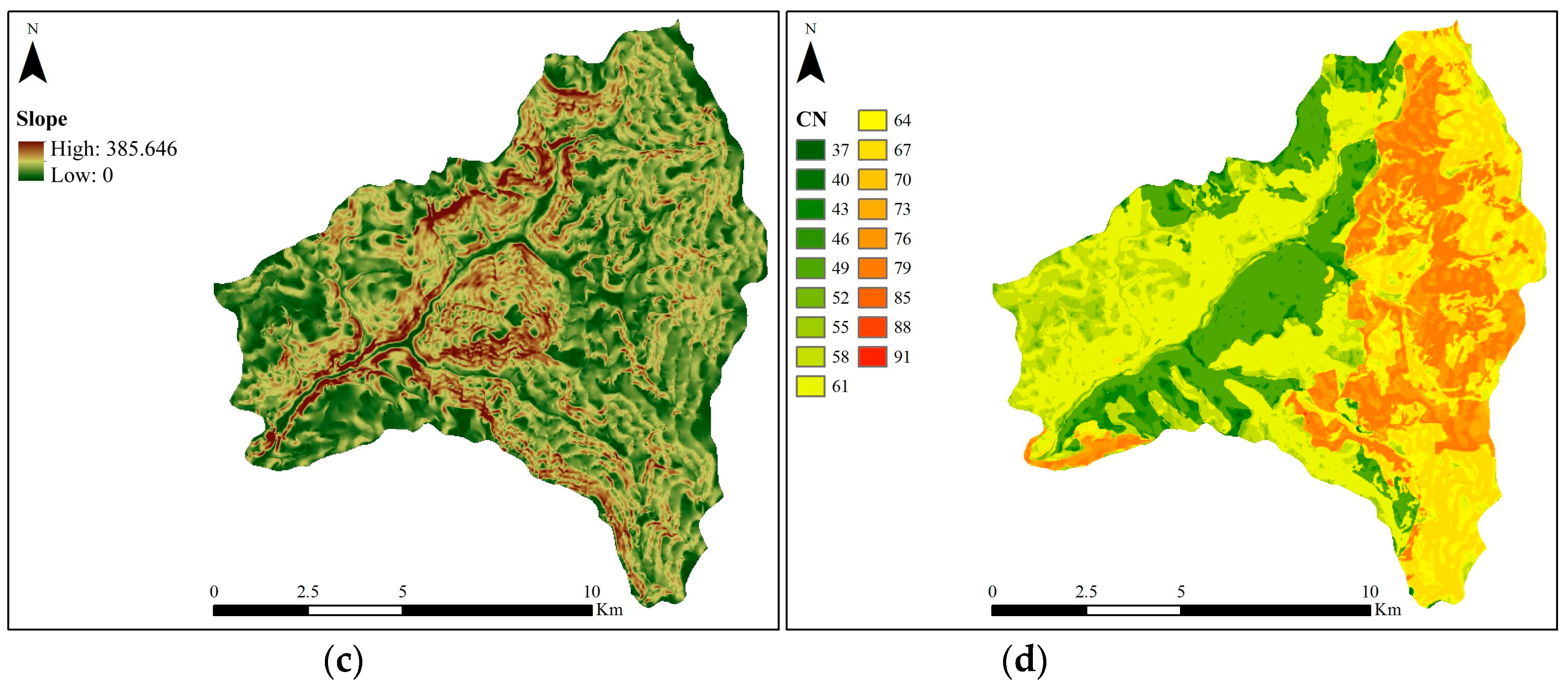
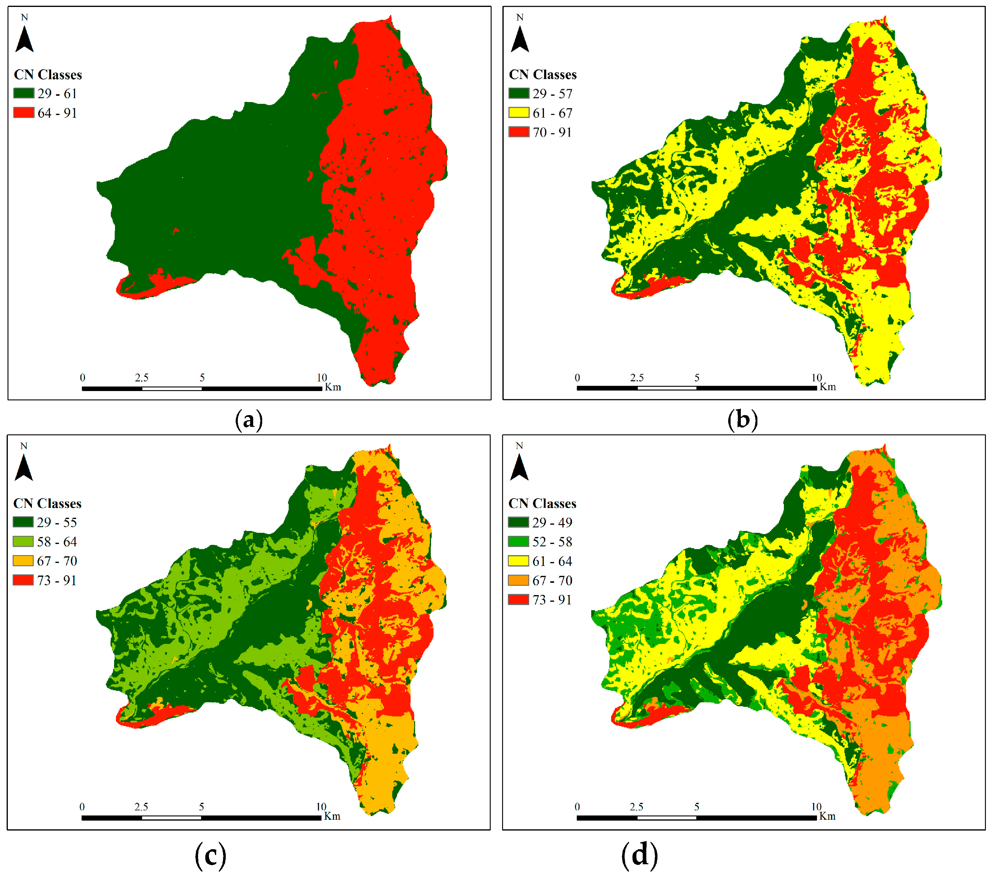
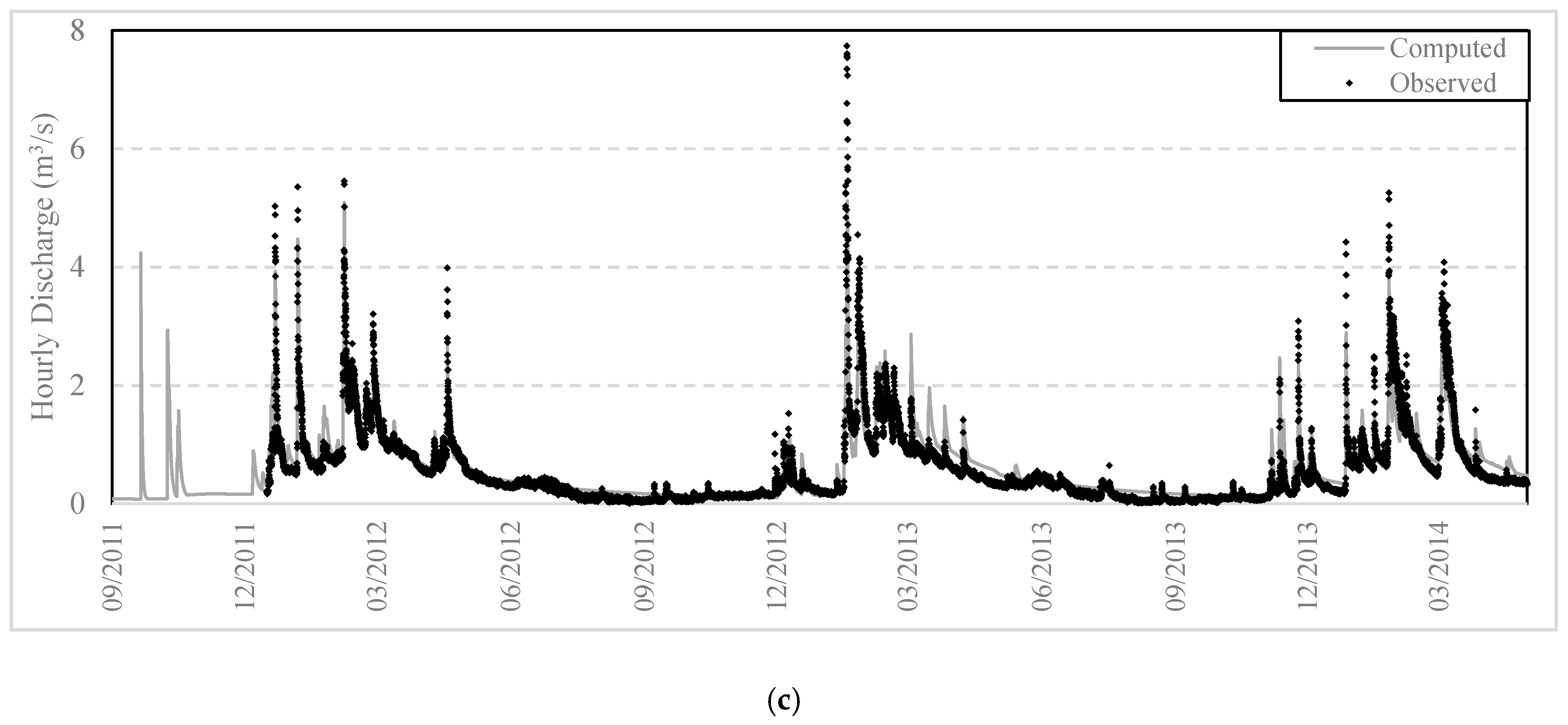
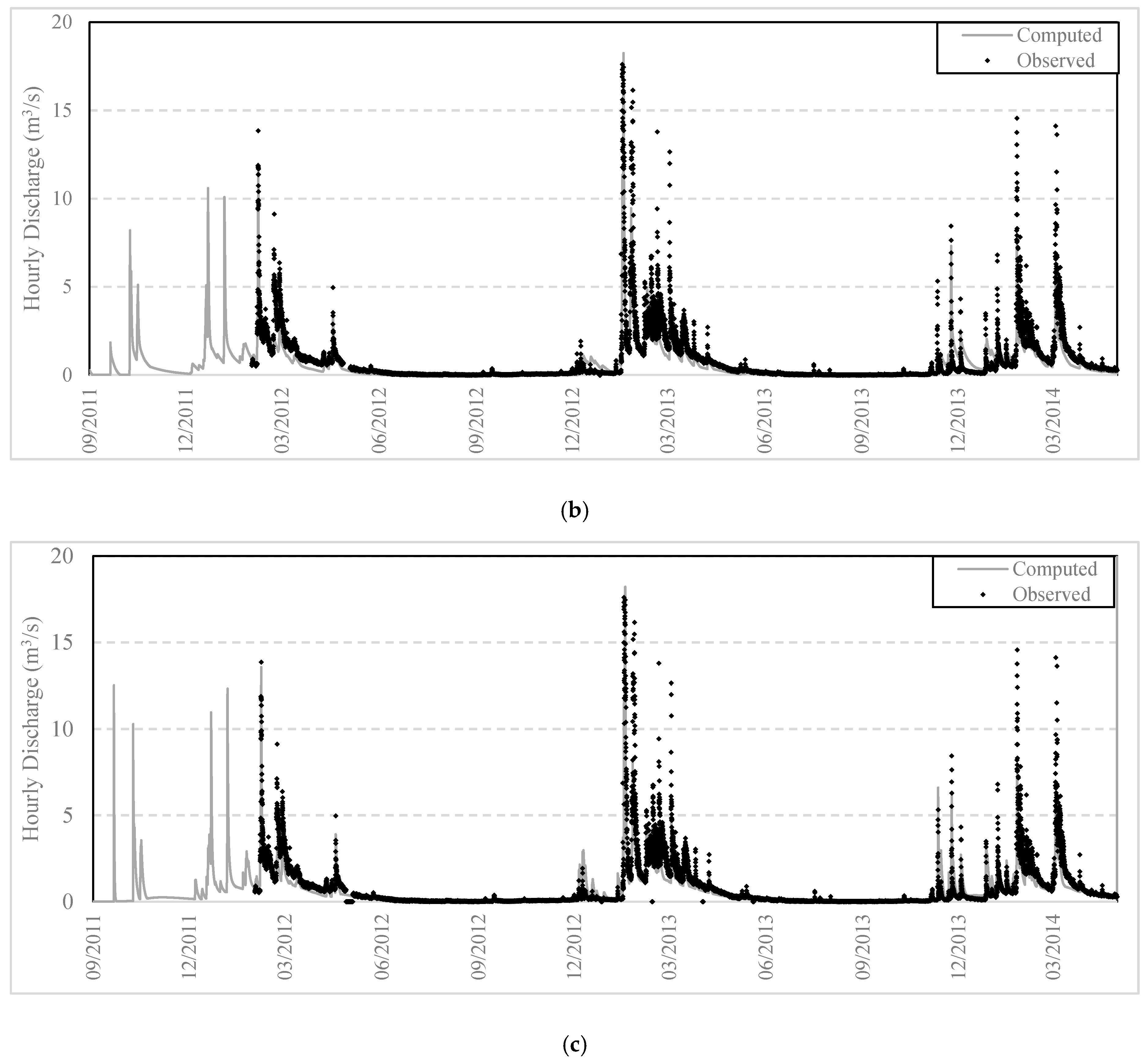
Table 1.
Coding of the physiographic characteristics for the estimation of parameter Curve Number (CN) for reference conditions (Antecedent Soil Moisture (AMC) Type II and initial abstraction ratio 20%).
Table 1.
Coding of the physiographic characteristics for the estimation of parameter Curve Number (CN) for reference conditions (Antecedent Soil Moisture (AMC) Type II and initial abstraction ratio 20%).
| Permeability Class | Vegetation Class | Drainage Capacity Class | |||
|---|---|---|---|---|---|
| Very high | 1 | Dense | 1 | Negligible | 1 |
| High | 2 | Moderate | 2 | Low | 2 |
| Moderate | 3 | Low | 3 | Moderate | 3 |
| Low | 4 | Sparse | 4 | High | 4 |
| Very low | 5 | Negligible | 5 | Very high | 5 |
Table 2.
Summary of flood data analysis at the pilot catchment of the DEUCALION project.
| Basin | Area (km2) | Examined Events | Average Runoff Coefficient | Average Observed CN (Adjusted) | Reference CN |
|---|---|---|---|---|---|
| Nedontas | 120.8 | 11 | 0.121 | 53 | 61 |
| Karveliotis | 15.3 | 10 | 0.171 | 52 | 65 |
| Alagonia | 20.9 | 10 | 0.350 | 74 | 70 |
| Lousios | 166.3 | 11 | 0.156 | 70 | 63 |
| Sarantapotamos | 144.6 | 12 | 0.059 | 62 | 48 |
| Oinoe | 51.2 | 12 | 0.012 | 52 | 45 |
| Chalandri stream | 5.2 | 1 | 0.215 | 88 | 62 |
| Drafi | 15.7 | 10 | 0.094 | 52 | 54 |
| Lykorema | 7.9 | 11 | 0.101 | 78 | 52 |
| Peristerona (Cyprus) | 77.1 | 14 | 0.407 | 72 | 71 |
| Xeros (Cyprus) | 68.5 | 10 | 0.279 | 70 | 66 |
Table 3.
Sub-basins properties.
| Sub-Basin | Name | Area (km2) | Mean Elevation (m) | Main Stream Length (m) | Mean Slope (%) |
|---|---|---|---|---|---|
| W60 | Nedousa | 19.47 | 1008.9 | 4296 | 23.1 |
| W180 | Alagonia | 20.72 | 1092.4 | 497 | 18.2 |
| W130 | Karveliotis | 14.92 | 1096.5 | 1721 | 21.2 |
| W170 | Downstream of Alagonia | 10.91 | 739.4 | 2807 | 20.3 |
| W120 | Downstream of Karveliotis | 11.81 | 710.1 | 5755 | 25.9 |
| W70 | Downstream of Nedousa | 12.53 | 741.9 | 4589 | 26.0 |
| W90 | Latomeio Baka | 28.2 | 654.8 | 5921 | 18.4 |
Table 4.
Overall model performance, expressed in terms of the composite error function, considering alternative parameterizations, by means of the number of HRUs.
Table 4.
Overall model performance, expressed in terms of the composite error function, considering alternative parameterizations, by means of the number of HRUs.
| HRUs | CN Classes | HRU Parameters | No. of Trials | Error Measure in Calibration | Error Measure in Validation |
|---|---|---|---|---|---|
| 1 | 29-91 | 7 | 2000 | 2.465 | 3.674 |
| 2 | 29–61 | 14 | 4000 | 2.072 | 3.043 |
| 64–91 | |||||
| 3 | 29–57 | 21 | 6000 | 1.985 | 2.675 |
| 61–67 | |||||
| 70–91 | |||||
| 4 | 29–55 | 28 | 8000 | 2.094 | 3.621 |
| 58–64 | |||||
| 67–70 | |||||
| 73–91 | |||||
| 5 | 29–49 | 35 | 10,000 | 2.390 | 3.519 |
| 52–58 | |||||
| 61–64 | |||||
| 67–70 | |||||
| 73–91 |
Table 5.
Optimal values of efficiency and high flow efficiency for varying numbers of HRUs.
| Hydrometric Station | Calibration Period | Validation Period | ||
|---|---|---|---|---|
| Efficiency | High Flow Efficiency | Efficiency | High Flow Efficiency | |
| One HRU | ||||
| Basin outlet: Latomeio Baka | 0.524 | 0.297 | 0.591 | −0.521 |
| Karveliotis | 0.672 | −0.166 | 0.687 | 0.218 |
| Alagonia | 0.662 | 0.054 | 0.708 | 0.416 |
| Two URHs | ||||
| Basin outlet: Latomeio Baka | 0.798 | 0.810 | 0.560 | −0.793 |
| Karveliotis | 0.887 | 0.676 | 0.712 | 0.259 |
| Alagonia | 0.674 | 0.083 | 0.722 | 0.496 |
| Three HRUs | ||||
| Basin outlet: Latomeio Baka | 0.672 | 0.722 | 0.706 | −0.067 |
| Karveliotis | 0.892 | 0.761 | 0.809 | 0.571 |
| Alagonia | 0.721 | 0.248 | 0.736 | 0.571 |
| Four HRUs | ||||
| Basin outlet: Latomeio Baka | 0.773 | 0.814 | 0.643 | −0.407 |
| Karveliotis | 0.869 | 0.631 | 0.738 | 0.285 |
| Alagonia | 0.673 | 0.145 | 0.724 | 0.513 |
| Five HRUs | ||||
| Basin outlet: Latomeio Baka | 0.716 | 0.762 | 0.567 | −0.563 |
| Karveliotis | 0.819 | 0.521 | 0.793 | 0.622 |
| Alagonia | 0.737 | 0.160 | 0.672 | 0.495 |
Table 6.
Number of HRUs and their parameters resulting from each delineation approach.
| Unique Combination | Union of Layers | CN Approach | |
|---|---|---|---|
| No. of HRUs | 31 | 4 | 3 |
| No. of HRU parameters | 217 | 28 | 21 |
| Total No. of parameters | 233 | 44 | 37 |
| Relative effort within hybrid calibration * | ~3 | ~1.5 | 1 |
Note: * Ranging from one to five, where 1 indicates minor and 5 major effort.
Table 7.
Optimal values of efficiency, high flow efficiency and average bias for three HRU delineation approaches.
Table 7.
Optimal values of efficiency, high flow efficiency and average bias for three HRU delineation approaches.
| Hourly Runoff | Calibration Period | Validation Period | ||
|---|---|---|---|---|
| Efficiency | High Flow Eff. | Efficiency | High Flow Eff. | |
| HRU delineation | Unique combination | |||
| Basin outlet: Latomeio Baka | 0.768 | 0.809 | 0.719 | 0.068 |
| Karveliotis | 0.908 | 0.663 | 0.813 | 0.580 |
| Alagonia | 0.754 | 0.253 | 0.680 | 0.141 |
| HRU delineation | Union of layers | |||
| Basin outlet: Latomeio Baka | 0.801 | 0.757 | 0.771 | 0.195 |
| Karveliotis | 0.655 | 0.693 | 0.762 | 0.368 |
| Alagonia | 0.658 | 0.090 | 0.726 | 0.411 |
| HRU delineation | CN based | |||
| Basin outlet: Latomeio Baka | 0.814 | 0.816 | 0.802 | 0.241 |
| Monitoring station: Karveliotis | 0.892 | 0.789 | 0.837 | 0.579 |
| Monitoring station: Alagonia | 0.797 | 0.300 | 0.753 | 0.440 |
Table 8.
Calibrated HRU parameters with the CN-based HRU delineation.
| HRU | CN 29–59 | CN 61–69 | CN 73–91 |
|---|---|---|---|
| Total Area (km2) | 40.2 | 54.8 | 22.9 |
| Max. infiltration ratio (mm/h) | 80.0 | 61.3 | 39.4 |
| Interception capacity (mm) | 50.0 | 39.4 | 5.0 |
| Soil capacity up to spill (mm) | 393.5 | 377.0 | 50.0 |
| Perc. of infiltration to the lower zone (%) | 78.8 | 54.083 | 5.292 |
| Soil capacity up to interflow (mm) | 500.0 | 428.4 | 110.6 |
| Recession rate for interflow (%) | 0.426 | 0.231 | 2.571 |
| Recession rate for percolation (%) | 0.187 | 0.116 | 0.055 |
Table 9.
Simulated water balance with the CN-based HRU delineation (mean annual values).
| Variable | Equivalent Depths (mm) | Volumes (hm3) | |
|---|---|---|---|
| Precipitation | 1690.3 | 200.1 | |
| Evapotranspiration | 623.0 | 73.8 | |
| Percolation | 607.1 | 71.9 | |
| Surface runoff | 385.5 | 45.6 | |
| Spring runoff | 249.6 | 29.6 | |
| Underground losses | 343.7 | 49.9 | |
| Soil storage change | 183.6 | 21.7 | |
| Groundwater storage change | 29.3 | 3.5 | |
| Outlet runoff | 557.2 | 66.0 | |
| (a) | |||
| Overall Water Balance | |||
| Output Variable | Percentage of Precipitation (%) | ||
| Evapotranspiration | 34.3 | ||
| River outflow | 30.7 | ||
| Underground losses | 23.2 | ||
| Storage change | 11.7 | ||
| (b) | |||
© 2018 by the authors. Licensee MDPI, Basel, Switzerland. This article is an open access article distributed under the terms and conditions of the Creative Commons Attribution (CC BY) license (http://creativecommons.org/licenses/by/4.0/).
Share and Cite
MDPI and ACS Style
Savvidou, E.; Efstratiadis, A.; Koussis, A.D.; Koukouvinos, A.; Skarlatos, D. The Curve Number Concept as a Driver for Delineating Hydrological Response Units. Water 2018, 10, 194. https://doi.org/10.3390/w10020194
AMA Style
Savvidou E, Efstratiadis A, Koussis AD, Koukouvinos A, Skarlatos D. The Curve Number Concept as a Driver for Delineating Hydrological Response Units. Water. 2018; 10(2):194. https://doi.org/10.3390/w10020194
Chicago/Turabian StyleSavvidou, Eleni, Andreas Efstratiadis, Antonis D. Koussis, Antonis Koukouvinos, and Dimitrios Skarlatos. 2018. "The Curve Number Concept as a Driver for Delineating Hydrological Response Units" Water 10, no. 2: 194. https://doi.org/10.3390/w10020194
Note that from the first issue of 2016, this journal uses article numbers instead of page numbers. See further details here.