Simulation of Groundwater Flow and Migration of the Radioactive Cobalt-60 from LAMA Nuclear Facility-Iraq

Abstract
:1. Introduction
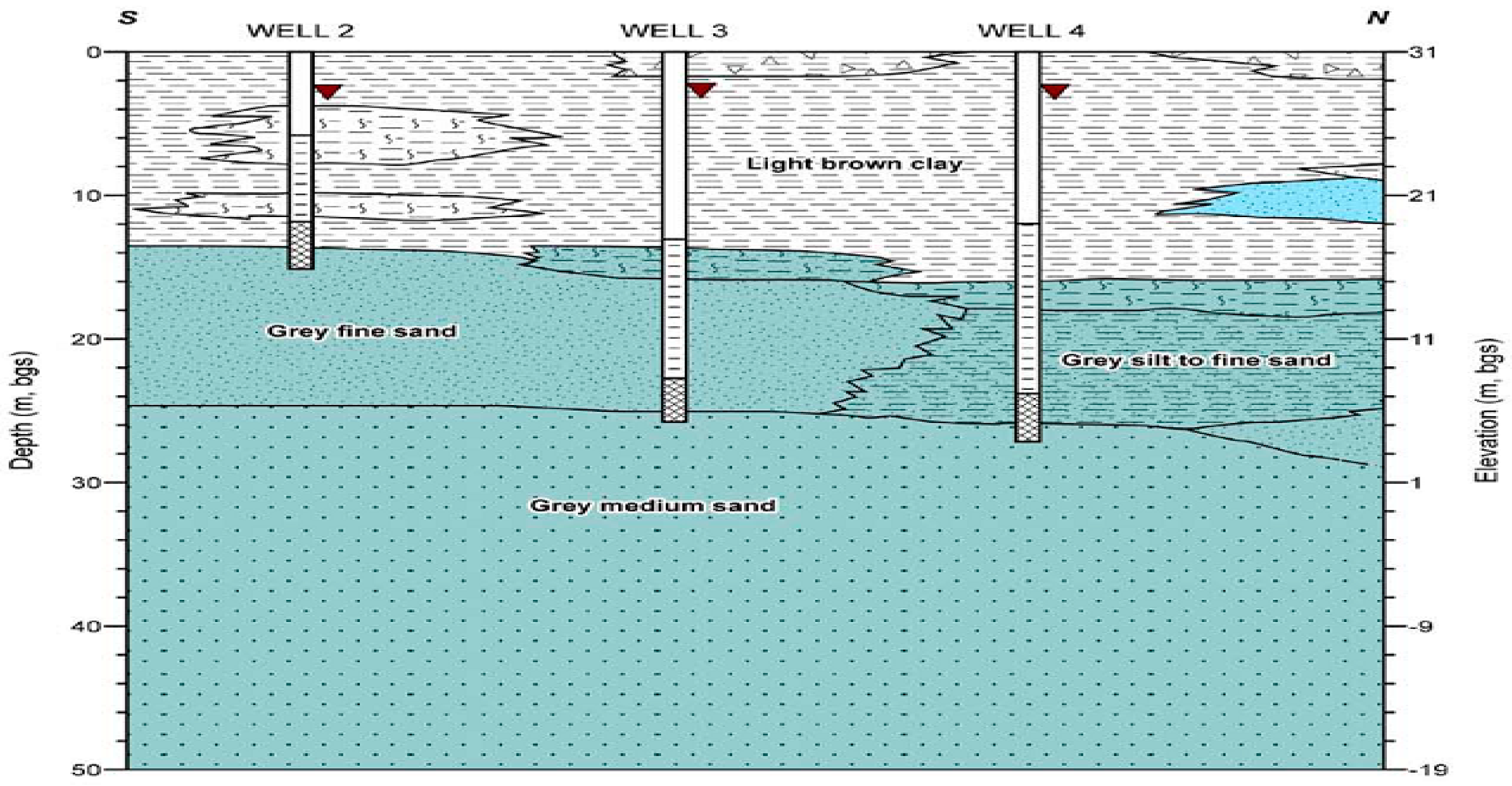
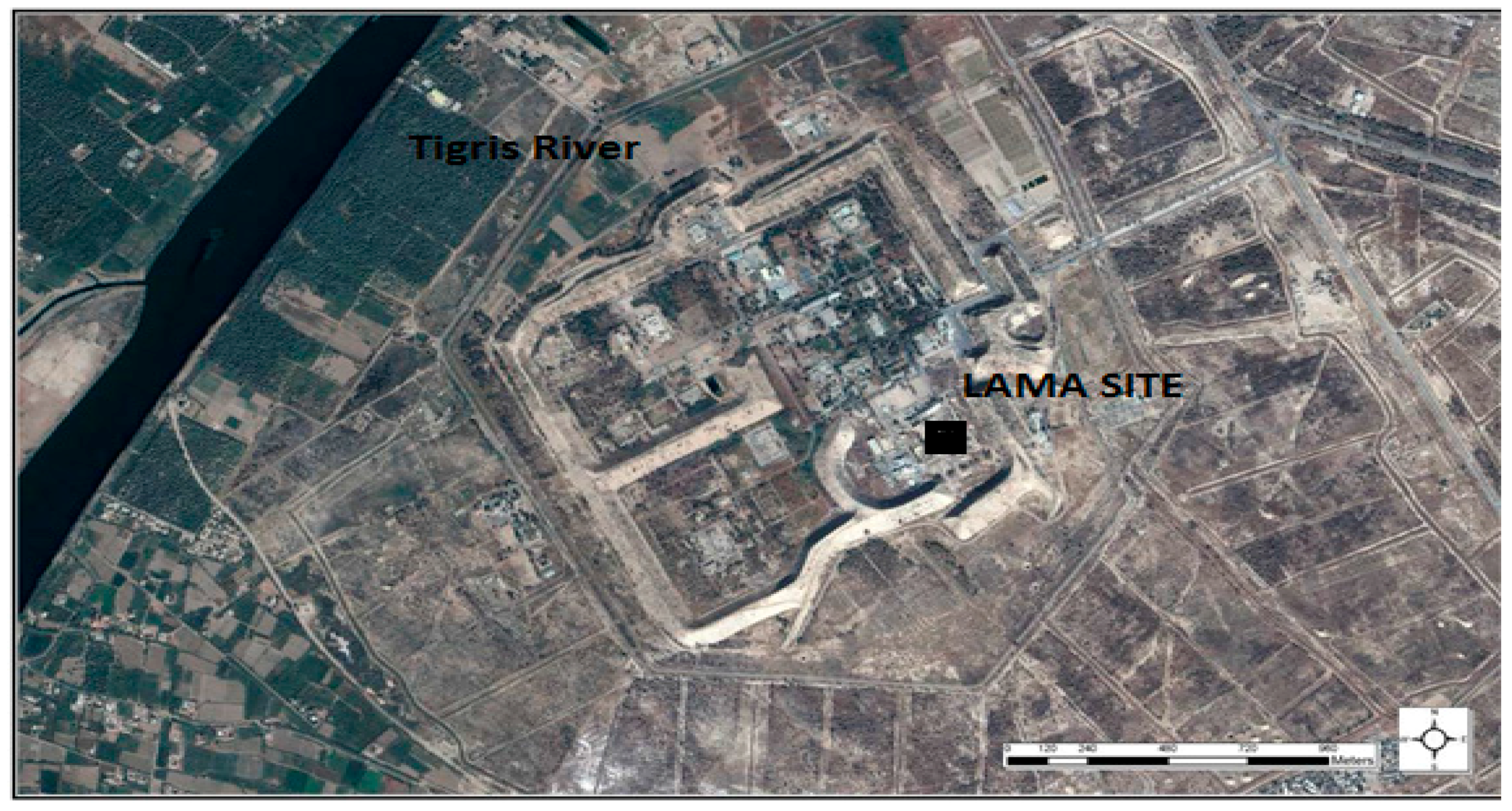
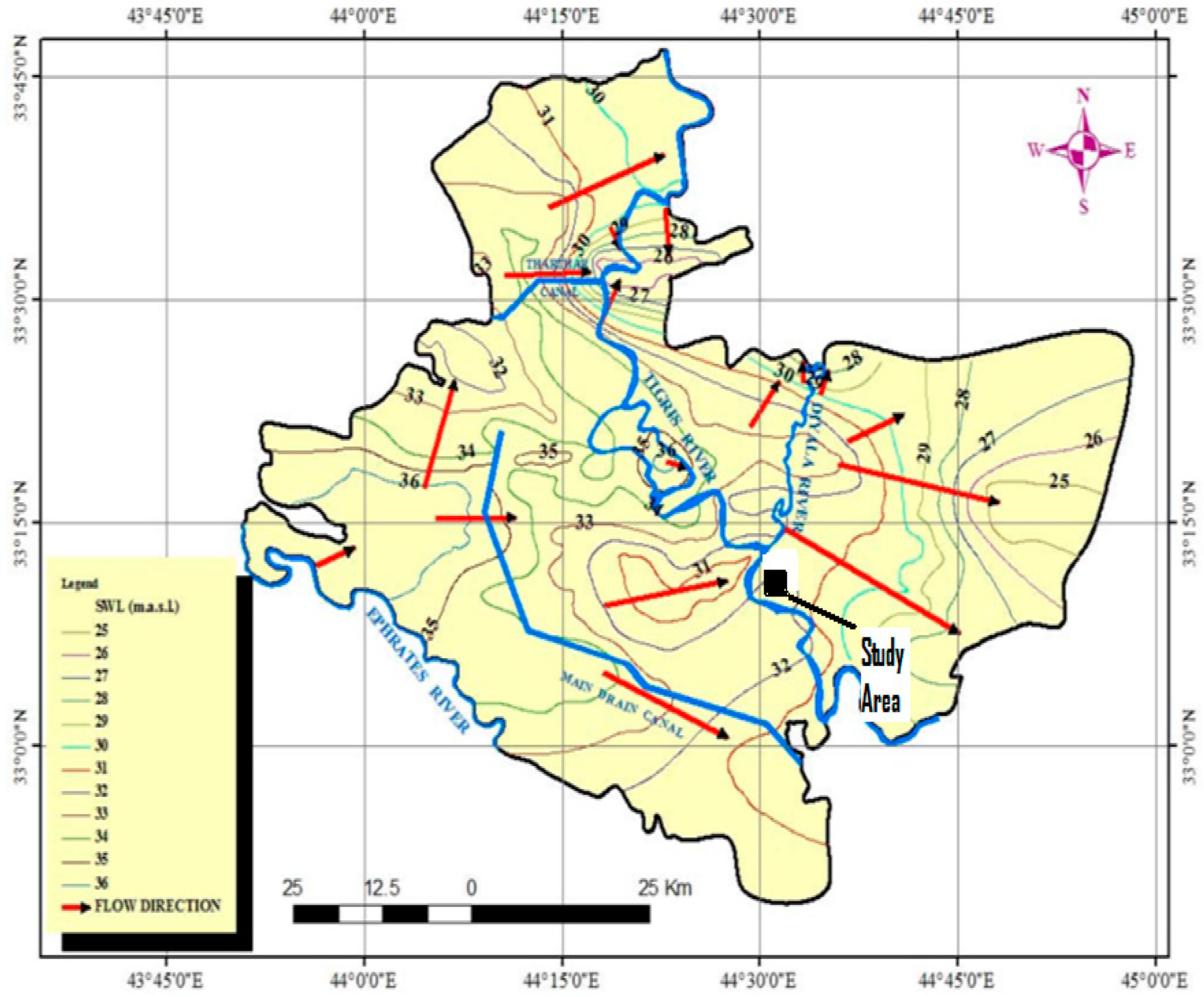
2. Study Area
3. Modeling of Groundwater Flow
3.1. The Governing Flow Equation
3.2. The Transport of Contaminant
- First order rate reaction (radioactive decay).
- Retardation factor (sorption–desorption reaction governed by a linear isotherm and constant distribution coefficient (Kd).
3.3. Groundwater Numerical Model
4. Methodology
4.1. Groundwater Flow Modeling
4.2. Cobalt-60 Transport
5. Results of Modeling
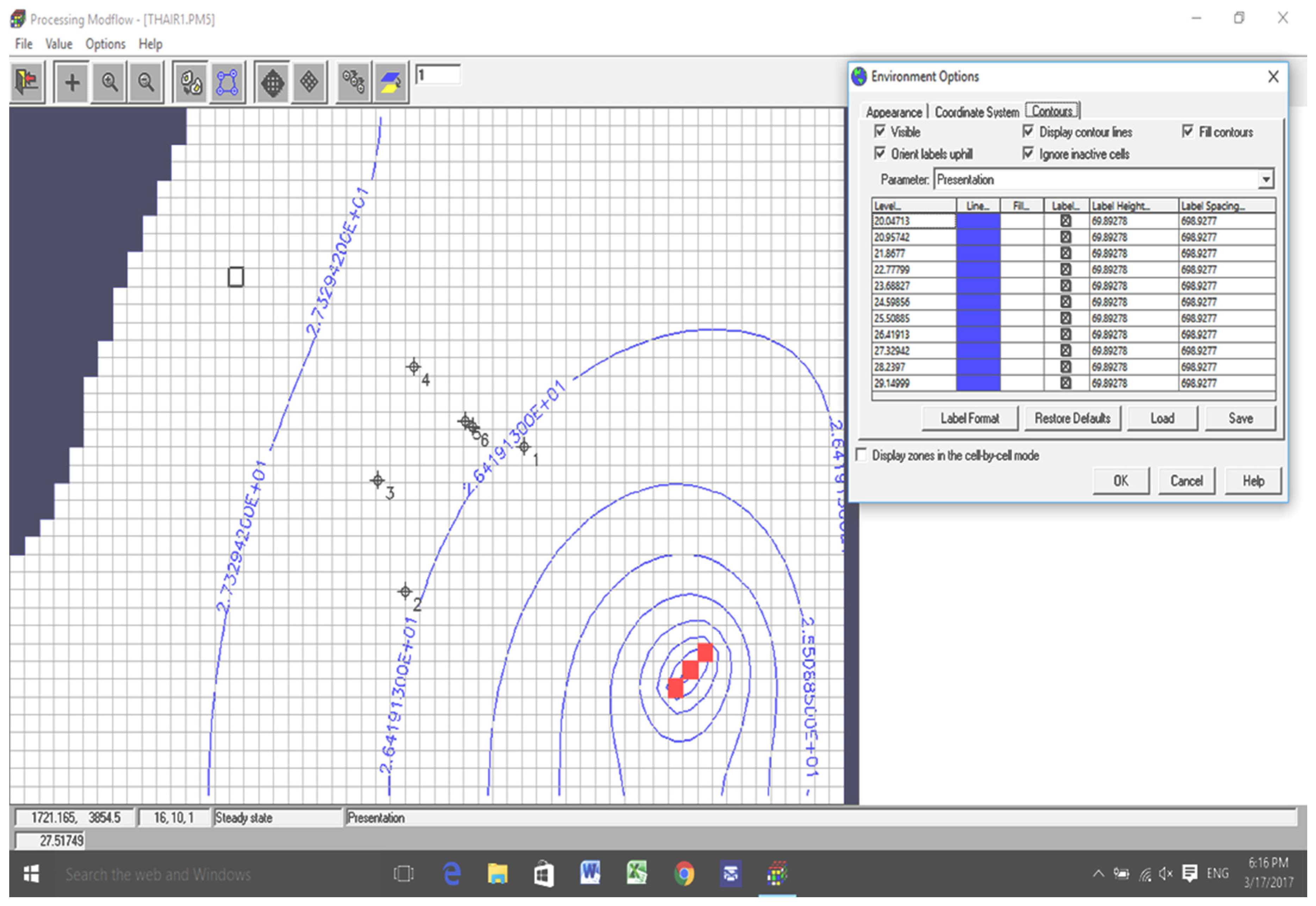
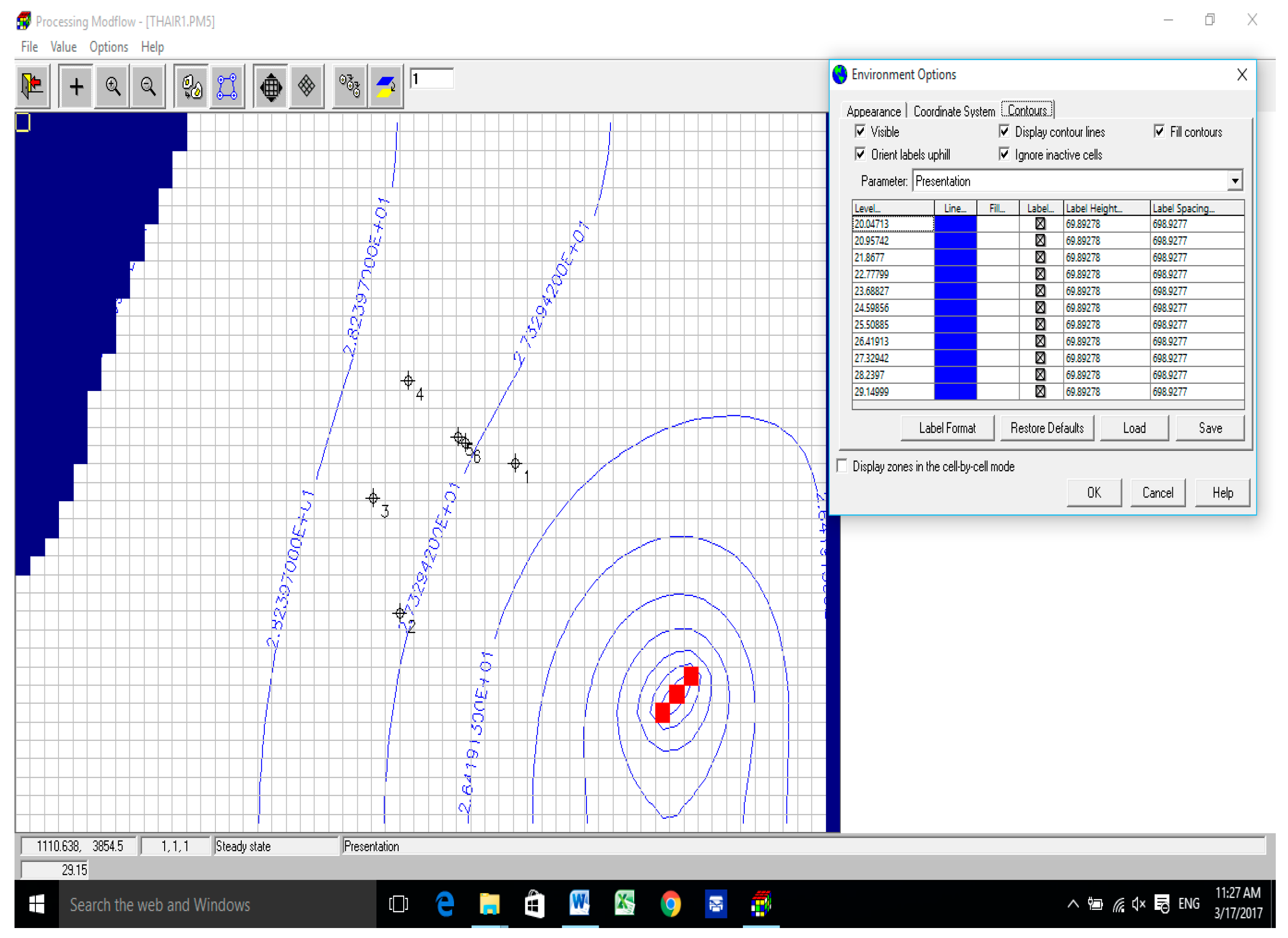
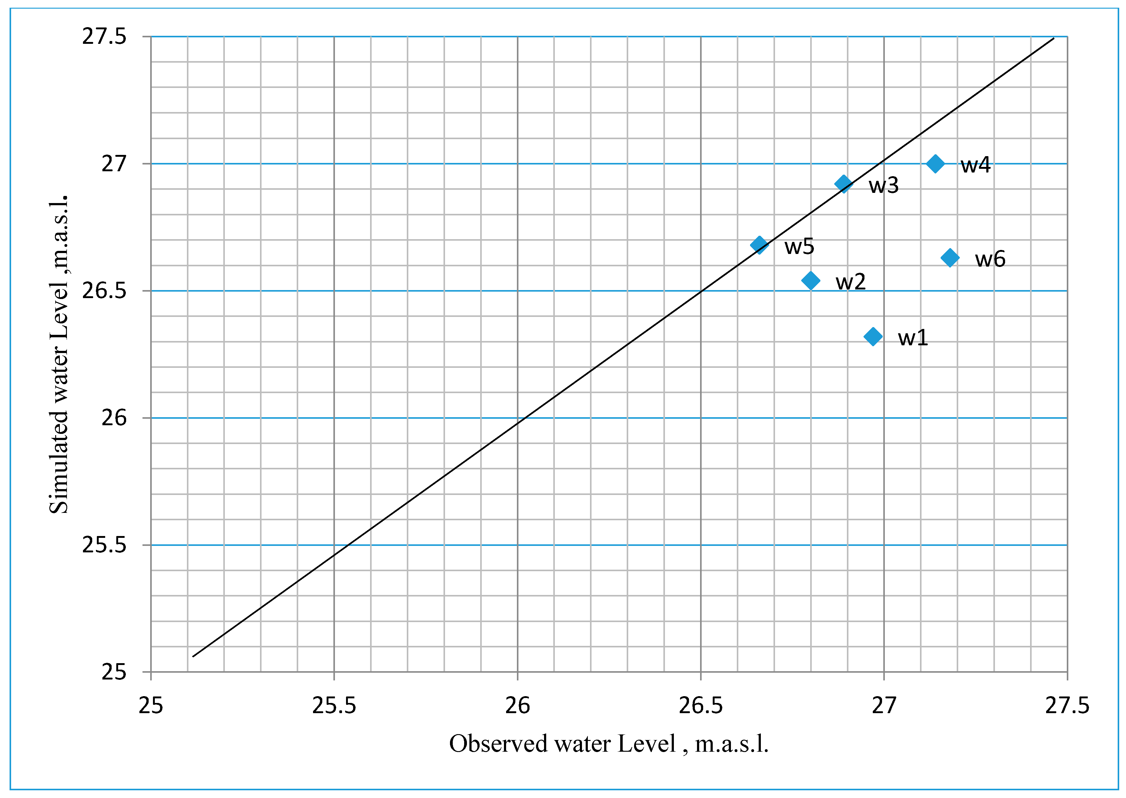
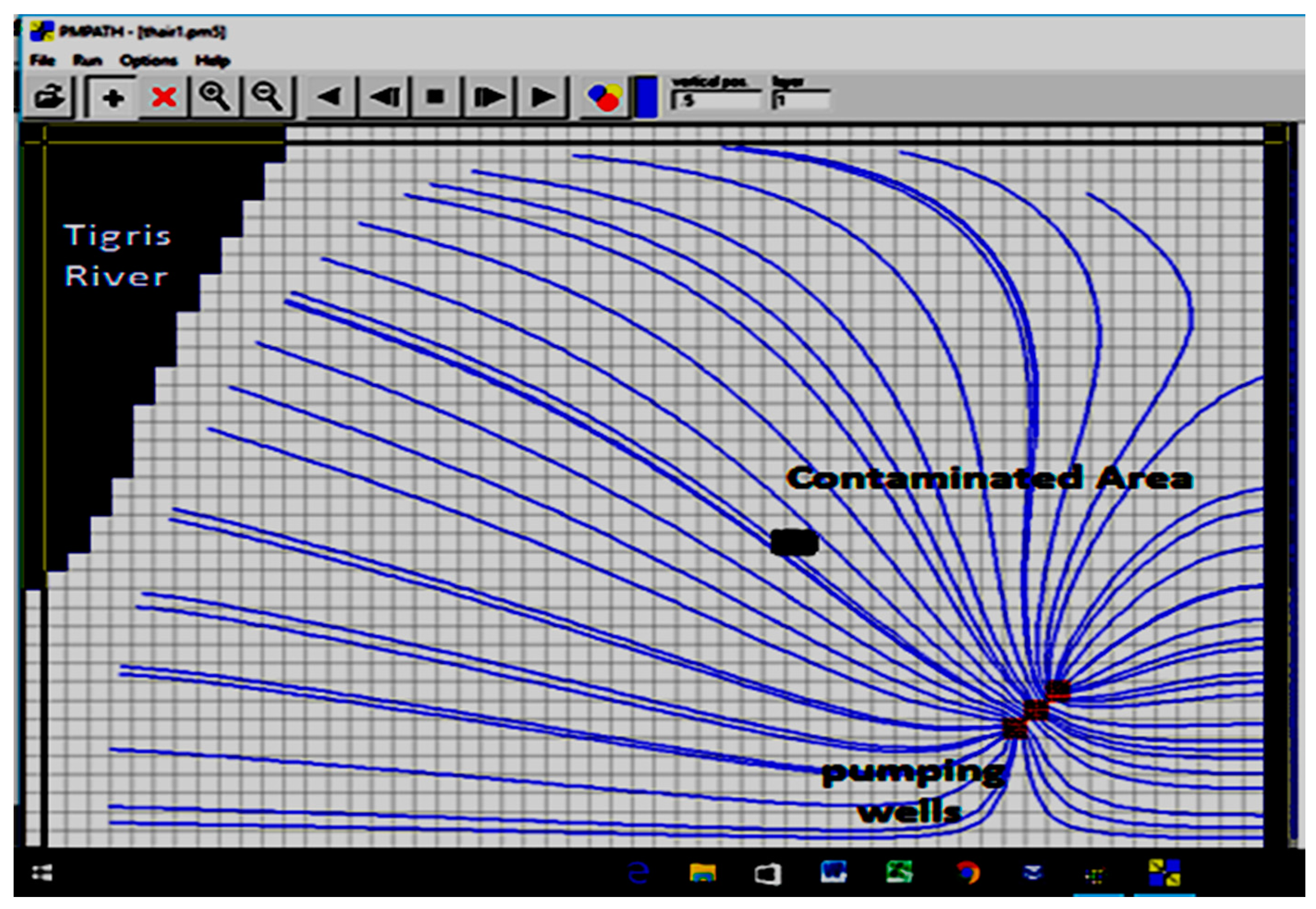
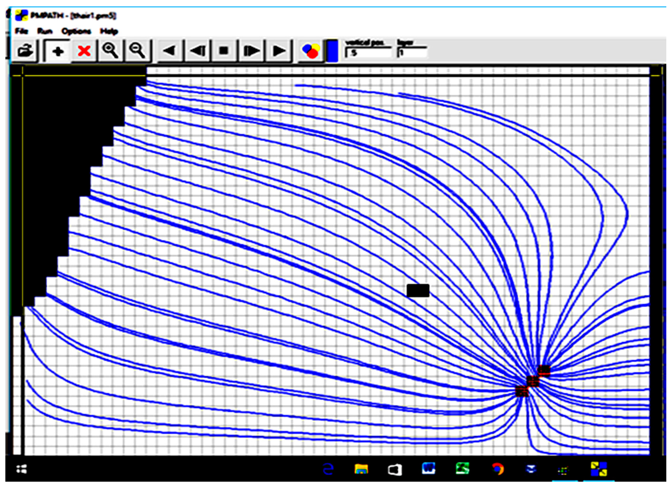
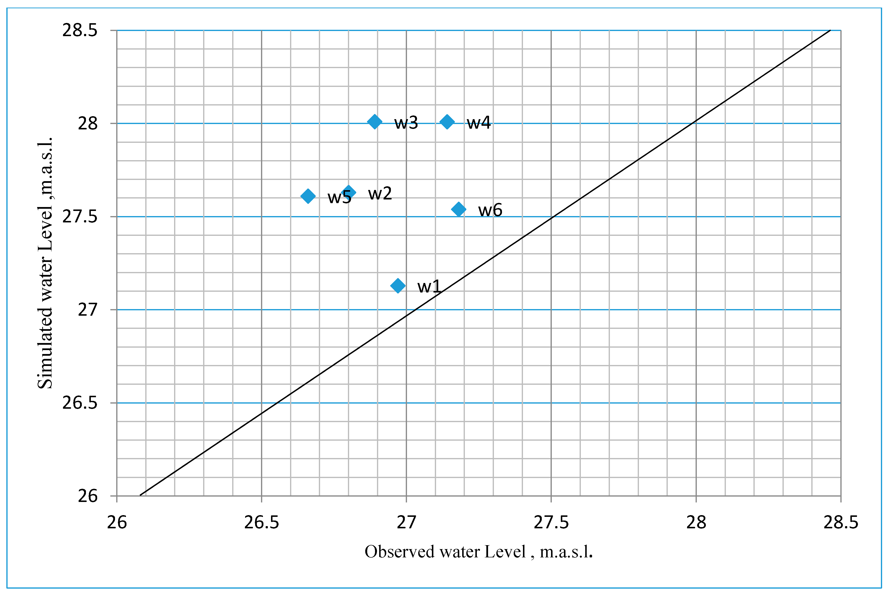
5.1. Groundwater Flow Modeling
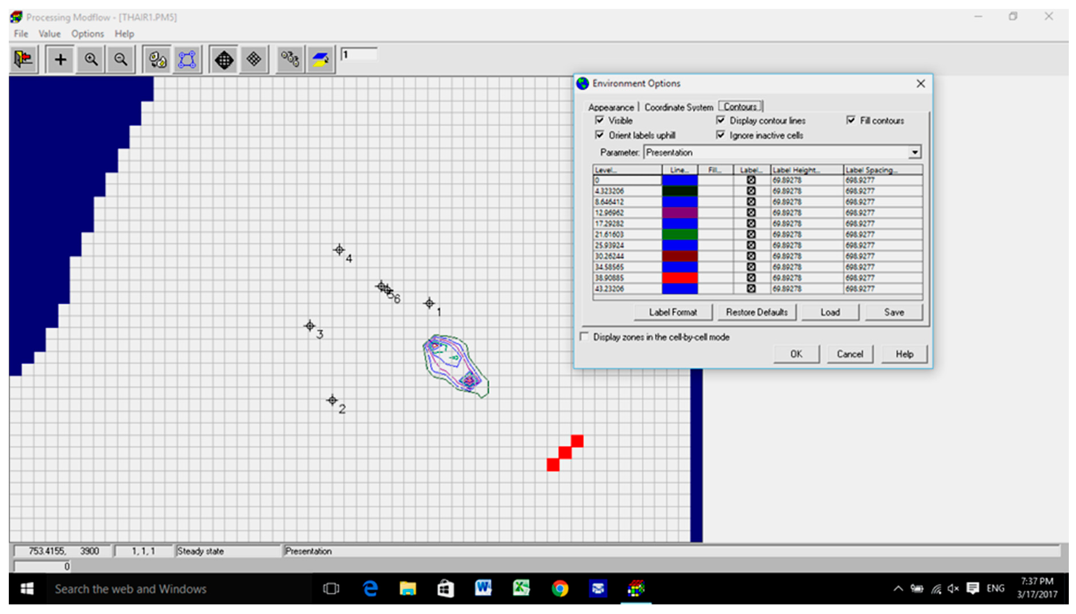
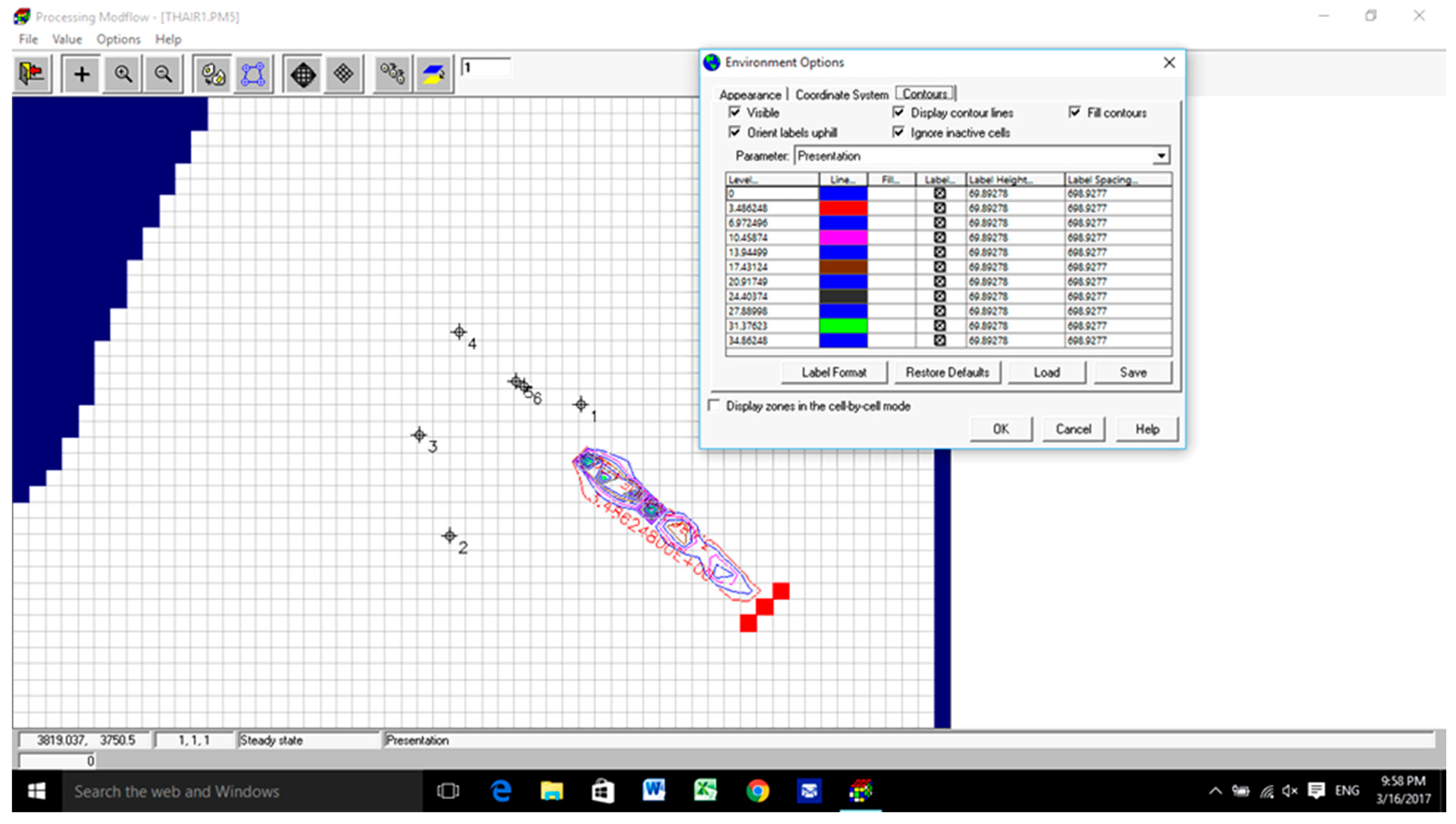
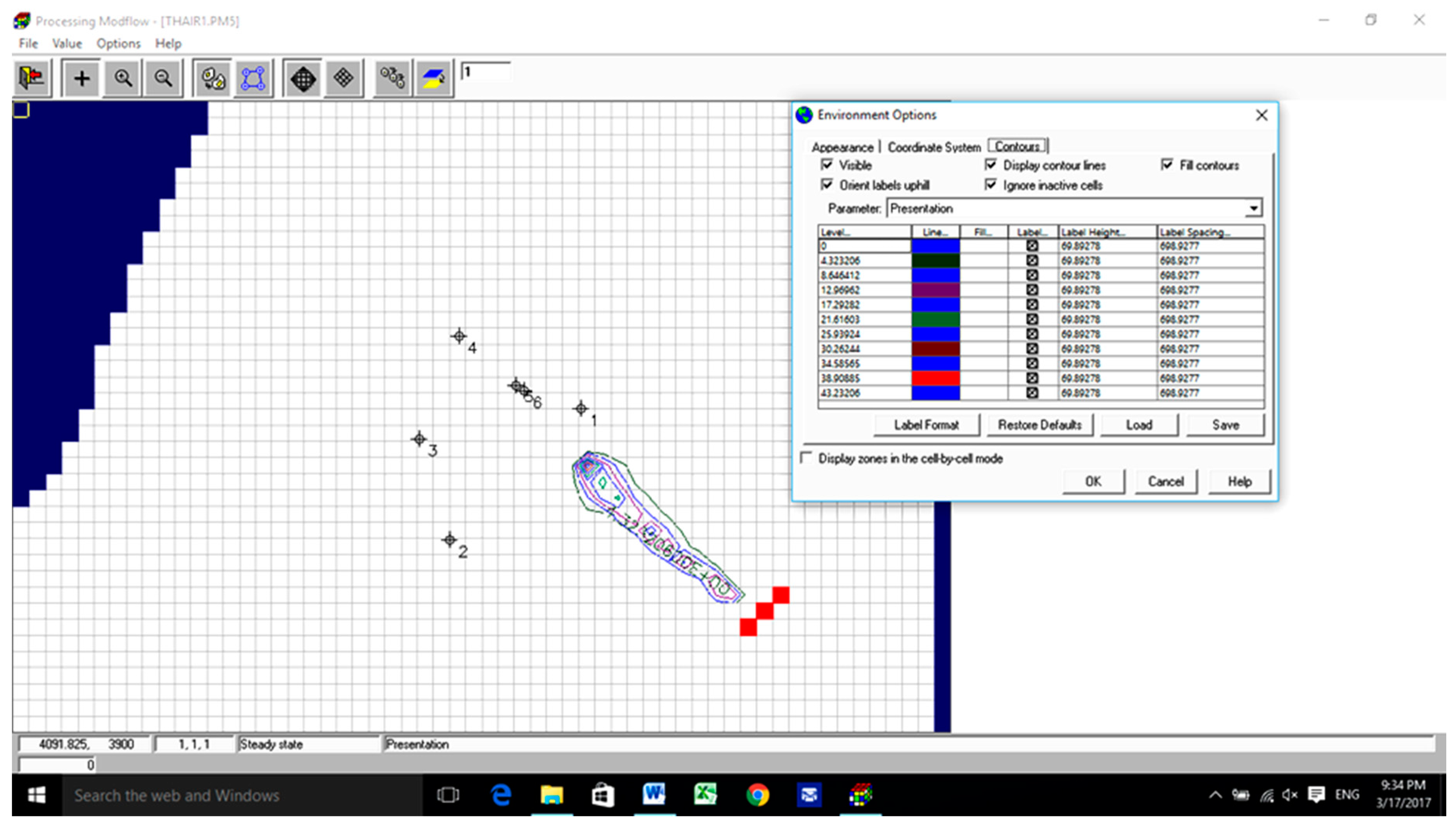
5.2. Co-60 Transport Modeling
6. Conclusions
Conflicts of Interest
References
- UNEP (United Nations Environment Program). Environmental in Iraq: UNEP Progress Report; United Nation Environment Program: Geneva, Switzerland, 2003. [Google Scholar]
- Sandia National Laboratories. Groundwater Monitoring Program Plan and Conceptual Site Model for Al-Tuwaitha Nuclear Research Center in Iraq; Sandia Report; Sandia National Laboratories: Livermore, CA, USA, 2013.
- IAEC (Iraq Atomic Energy Commissio). Piecing Together Iraq’s Nuclear Legacy; Bulletin of the Atomic Scientists: Chicago, IL, USA, 1991. [Google Scholar]
- Eliezer, J.W. Groundwater Flow and Solute Transport at a Municipal Landfill Site on Long Island; Water Resources Investigations Report, 86-4207; U.S. Geological Survey: New York, NY, USA, 1988.
- Ramzi, M. Shihab Modeling of Cs-137 and Co-60 Transport in Calcareous Soils by Groundwater. J. Soil Sci. Environ. Manag. 2014, 5, 52–61. [Google Scholar]
- Grey, P.; Ahmed, E. Modeling Groundwater Flow and Radioactive Transport in a Fractured Aquifer; Water Resources Center: Las Vegas, NV, USA, 1999; Volume 37. [Google Scholar]
- NEI (Nuclear Energy Institute). Industry Groundwater Protection Initiative; Final Guidance Document; Nuclear Energy Institute: Washington, DC, USA, 2007.
- Abbas, M.J.; Latif, K.H.; Ahmed, B.A. Groundwater Monitoring Program at AL-Tuwaitha Nuclear Research Center, Iraq; Informal Paper; National Nuclear Security Administration: Washington, DC, USA, 2010; p. 21.
- Peter, W. A Non-Technical Guide to Groundwater Modeling; U.S. Department of Energy Hanford Site: Washington, DC, USA, 2007.
- Bear, J. Hydraulics of Groundwater; McGraw-Hill: New York, NY, USA, 1979; p. 569. [Google Scholar]
- Jacques, W. The Handbook of Groundwater Engineering; School of Civil Engineering, Purdue University: West Lafayette, IN, USA, 1999. [Google Scholar]
- Grove, D.B. Derivation of Equations Describing Solute Transport in Groundwater; U.S. Geological Survey, Water Resources Investigations: New York, NY, USA, 1976.
- Domenico, P.A.; Schwartz, F.W. Physical and Chemical Hydrogeology; John Wiley and Sons: New York, NY, USA, 1990; p. 709. [Google Scholar]
- Schulze-Makuch, D. Longitudinal Dispersivity Data and Implications for Scaling Behavior. Groundwater 2005, 43, 443–456. [Google Scholar] [CrossRef] [PubMed]
- Larry, M.; Terry, S. Sorption Kd Measurements on Cinder Block and Grout in Support of Dose Assessments for Zion Nuclear Station Decommissioning; Informal Report; Environmental and Climate Sciences Department, Brookhaven National Laboratory: New York, NY, USA, 2014.
- Naseer, H. Evaluation of the Groundwater in Baghdad Governorate-Iraq. J. Sci. 2015, 56, 1708–1718. [Google Scholar]
- Al-Adili, A.; Ali, S. Hydro-Chemical Evolution of Shallow Groundwater System within Baghdad City-Iraq. In Proceedings of the Tenth International Water Technology Conference (IWTC10 2006), Alexandria, Egypt, 23–25 March 2006; pp. 23–25. [Google Scholar]
- Ministry of Water Resources—Iraq. Flow Rates of Water in Tigris River; Report; National Center for Water Resources Management: Baghdad, Iraq, 2015.
- Bashoo, D.; Lazim, S.; Alwan, M. Hydrogeology of Baghdad Province; Internal Report; General Directorate of Water Well Drilling: Baghdad, Iraq, 2005. [Google Scholar]
- ICRP (International Commission on Radiological Protection). Guidelines for Drinking Water Quality; World Health Organization: Geneva, Switzerland, 1991. [Google Scholar]
- Al-Musawi, F. Radioactive Waste Management Policy and Strategy in Iraq; Deputy Minister, Ministry for Science and Technology: Baghdad, Iraq, 2010; p. 24. [Google Scholar]
- Perry, M.J. Characterization of Groundwater Flow Surrounding Aquifers; Water Resources Investigations Report, 02-4198; U.S. Geological Survey: Mound View, MN, USA, 2002; p. 24.


| Year | Well No. | |||||
|---|---|---|---|---|---|---|
| 1 | 2 | 3 | 4 | 5 | 6 | |
| Dry season 2011 | 26.20 | 26.00 | 26.25 | 26.50 | 25.70 | 26.60 |
| Wet season 2011 | 26.90 | 26.70 | 26.83 | 27.10 | 26.24 | 27.10 |
| 2002 | 27.80 | 27.70 | 27.60 | 27.81 | 28.05 | 27.85 |
| Average | 26.97 | 26.8 | 26.89 | 27.14 | 26.66 | 27.18 |
| Layer | Depth m | Soil | KH cm/s | Bulk Density kg/m3 | Effective Porosity % |
|---|---|---|---|---|---|
| 1 | 16 | Light brown clay | 10−8–10−5 | 1200–1500 | 1–18 |
| 2 | 10 | Grey silt to fine sand | 10−5–10−3 | 1400–1600 | 1–39 |
| 3 | 24 | Grey medium sand | 10−3–10−1 | 1600–1700 | 16–46 |
| Layer | Soil | Hydraulic Conductivity | Effective Porosity | ||
|---|---|---|---|---|---|
| Default Value cm/s | Calibrated Value cm/s | Default Value % | Calibrated Value % | ||
| 1 | Light brown clay | 10−8–10−5 | 5 × 10⁻⁷ | 1–18 | 16 |
| 2 | Grey silt to fine sand | 10−5–10−3 | 1 × 10⁻⁴ | 1–39 | 28 |
| 4 | Grey medium sand | 10−3–10−1 | 3 × 10⁻² | 16–46 | 35 |
© 2018 by the author. Licensee MDPI, Basel, Switzerland. This article is an open access article distributed under the terms and conditions of the Creative Commons Attribution (CC BY) license (http://creativecommons.org/licenses/by/4.0/).
Share and Cite
Khayyun, T.S. Simulation of Groundwater Flow and Migration of the Radioactive Cobalt-60 from LAMA Nuclear Facility-Iraq. Water 2018, 10, 176. https://doi.org/10.3390/w10020176
Khayyun TS. Simulation of Groundwater Flow and Migration of the Radioactive Cobalt-60 from LAMA Nuclear Facility-Iraq. Water. 2018; 10(2):176. https://doi.org/10.3390/w10020176
Chicago/Turabian StyleKhayyun, Thair Sharif. 2018. "Simulation of Groundwater Flow and Migration of the Radioactive Cobalt-60 from LAMA Nuclear Facility-Iraq" Water 10, no. 2: 176. https://doi.org/10.3390/w10020176
APA StyleKhayyun, T. S. (2018). Simulation of Groundwater Flow and Migration of the Radioactive Cobalt-60 from LAMA Nuclear Facility-Iraq. Water, 10(2), 176. https://doi.org/10.3390/w10020176