Improving Stochastic Modelling of Daily Rainfall Using the ENSO Index: Model Development and Application in Chile

Abstract

Stochastic weather simulation, or weather generators (WGs), have gained a wide acceptance and been used for a variety of purposes, including climate change studies and the evaluation of climate variability and uncertainty effects. The two major challenges in WGs are improving the estimation of interannual variability and reducing overdispersion in the synthetic series of simulated weather. The objective of this work is to develop a WG model of daily rainfall, incorporating a covariable that accounts for interannual variability, and apply it in three climate regions (arid, Mediterranean, and temperate) of Chile. Precipitation occurrence was modeled using a two-stage, first-order Markov chain, whose parameters are fitted with a generalized lineal model (GLM) using a logistic function. This function considers monthly values of the observed Sea Surface Temperature Anomalies of the Region 3.4 of El Niño-Southern Oscillation (ENSO index) as a covariable. Precipitation intensity was simulated with a mixed exponential distribution, fitted using a maximum likelihood approach. The stochastic simulation shows that the application of the approach to Mediterranean and arid climates largely eliminates the overdispersion problem, resulting in a much improved interannual variability in the simulated values.

1. Introduction

Climate records are used for a wide variety of purposes, ranging from the characterization of climatic types of a particular location, to running operational models for resource evaluation and exploitation [1]. Climate data are also relevant for agricultural and ecological research [2,3], becoming critical inputs to forecast crop growth and development rates, as well as to model population dynamics of pest and diseases [4]. In addition, the data represent a baseline to assess global and local climate change effects [5]. However, climate information is not always available with the required spatial resolution and temporal coverage. Such lack of information becomes worse as one tries to retrieve information from the past. As an example, only 65% of the daily precipitation data in Chile can be retrieved for 2013, whereas less than 5% of daily rainfall data from 1950 is available (Figure 1). Thus, obtaining a complete and reliable long-term historical climate series is typically a challenge.

Stochastic weather models, or weather generators (WGs), are algorithms to generate synthetic series of climate variables, preserving the main statistical parameters of the observed series. WGs can effectively represent the intrinsic natural variability of the rainfall process, which is a prominent issue in the analysis of the projected uncertainties. The three main applications of WGs are (1) modelling weather and climate-sensitive systems, (2) generating missing weather data, and (3) downscaling global and regional climate change scenarios [6]. One of the first WGs was presented by Richardson (1981) [7], who developed an algorithm to simulate daily precipitation, radiation, and maximum and minimum temperature. This model was implemented as WGEN (Weather GENerator) by Richardson and Wright (1984) [1], which used a simple Markov Chain for precipitation occurrence, a gamma distribution for simulation of rainfall amounts, and an autoregressive model for the remaining variables. A number of subsequent WGs, such as WXGEN [8], CLIGEN [9,10], LARS-WG [11,12,13], ClimGen [14], WeaGETS [15,16], Met and Roll [17], MOFRBC [18,19], WeatherMan [20], MarkSim [21], AAFC-WG [22,23], WM2 [24], KnnCAD [25,26,27], and the WG used by the UK Met Office (UKCP09) [28,29], all share the basic principles of stochastic simulation presented in WGEN. These WGs are station-scale generators, with time scales that range from daily (or even hourly in the case of rainfall) to annual, daily resolution being the most common.

In recent years, most of the efforts in the improvement of WGs have been focused on the representation of daily rainfall, which can affect the simulation of the other climate variables [30]. The application of WGEN in Chile, Taulis, and Milke [31] reported an underestimation of the annual precipitation of 42% in arid region, and identified gaps to be addressed in order to assemble a new and better stochastic model. Also, Lobo et al. [10] used CLIGEN (CLImate GENerator) in central Chile (32°–39° S), and found that prior to calibration, the storm durations and maximum intensities were consistently overestimated and underestimated, respectively, especially in the wet season.

An alternative to improve the stochastic estimation of daily rainfall is to incorporate a generalized lineal model (GLM), with logistic regressions or logistic functions for the occurrences (binary process). Sometimes this approach is also adopted for the simulation of precipitation intensity, especially when the aim is to represent rainfall values that are clearly non-Gaussian [32]. The use of GLM was first proposed by Stern and Coe [33] and later, further developed by Yang et al. [34] and Chandler [35]. A GLM approach in WGs has been used by Verdin et al. [36] with fairly good results. Furrer and Katz [37] argue that its use can lead to a substantial improvement in the simulation of extreme precipitation, with several possible approaches (e.g., a hybrid technique with a gamma distribution for low to moderate intensities, and a generalized Pareto distribution for high intensities).

Another open area of research is the development and assessment of models to address the overdispersion phenomenon, i.e., when the observed variance exceeds that of the simulated values (e.g., Kim et al. [38] and Katz and Parlange [39]), and the improvement of the representation of interannual variability, by incorporating additional variables into the GLM scheme. For example, the El Niño–Southern Oscillation (ENSO) phenomenon is a large-scale atmospheric–oceanic feature that explains an important fraction of climate variability in several parts of the world [40,41]. Part of the fluctuations in the climatic regime of central Chile can be associated with this phenomenon. In fact, abundant precipitation is observed when the El Niño phase is present, while lower precipitation is expected during La Niña events [42].

Considering the potential for improvement associated with the use of covariables for the representation of interannual variability in a GLM approach, our aim is to develop a stochastic weather generator to model daily precipitation, incorporating ENSO index as a covariable. Furthermore, the model considers a mixed exponential distribution for simulating highly variable and skewed rainfall. Such an algorithm can be easily implemented and incorporated into existing WGs models. The proposed model is applied to a set of daily rainfall series observed in gauges located in arid, Mediterranean, and temperate (Wet) climates in Chile. This study discusses some of the issues encountered, to estimate the main set of parameters and propose recommendations for the future development of WGs.

2. Materials and Methods

This study seeks to develop a stochastic weather generator capable of reproducing precipitation series from several climatic zones. In our experiment, we developed two models, one with and one without ENSO, to evaluate ENSO’s relevance as a covariable. We applied the models across the continental area of Chile, covering a wide range of precipitation regimes from North to South that can be broadly classified into arid, Mediterranean, and temperate (Wet) types. The arid regime with coastal influence, represented here by the location of La Serena, presents a short rainy season from July to August. In this region, overcast skies, small rainfall amounts, and relatively colder temperatures are frequent. However, in the interior area (i.e., Copiapó and Vallenar) the presence of the desert results in arid, clear skies, and low relative humidity. The Mediterranean regime presents a rainy season concentrated in winter (from June to August), mainly driven by the influence of the South Tropical Anticyclone (SPA) and the cold Humboldt current along the Pacific coast [43]. The main source of interannual variability is El Niño Southern Oscillation (ENSO), producing typically above and below normal precipitation during El Niño and La Niña periods, respectively. In fact, Montecinos y Aceituno [44] argues that during El Niño episodes, above-average annual precipitation tends to occur over the region 35° to 38° S in late spring (October–November). In the temperate climate, rainfall is consistently present throughout the year. The effect of ENSO in areas with marked although above normal precipitation is expected during very strong El Niño periods. Note that during the 20th century, the subtropical zone (30°–37° S) of Chile has experienced a significant reduction in precipitation [45]. This decrease is mainly reflected in annual and winter precipitation in the Mediterranean region (30°–33° S), with periods of more precipitation between 1900–1940 and 1970–2000 (although not significant) [46], and a marked negative precipitation trend and high interannual variability during the period 1940–1970 [47].

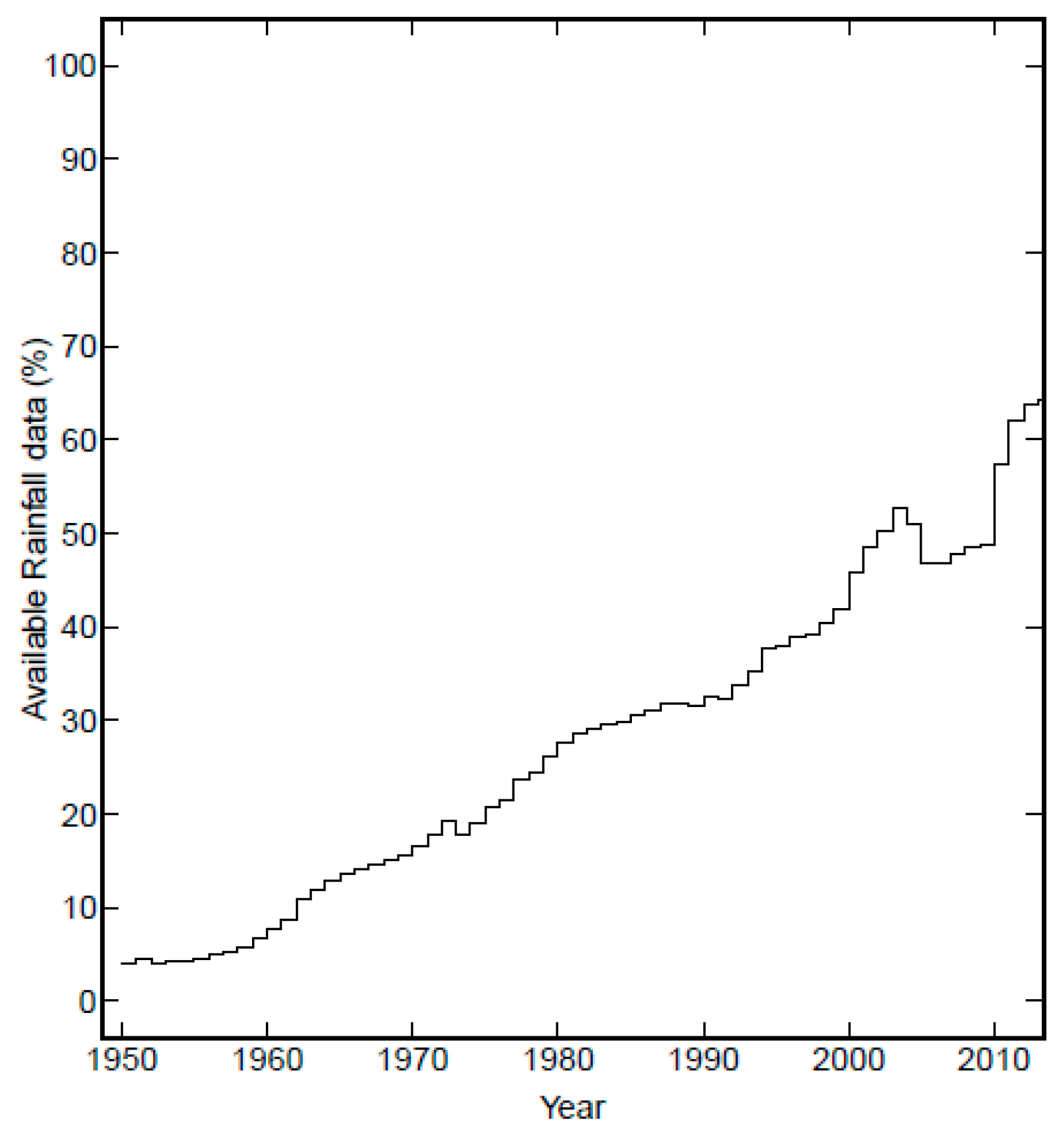
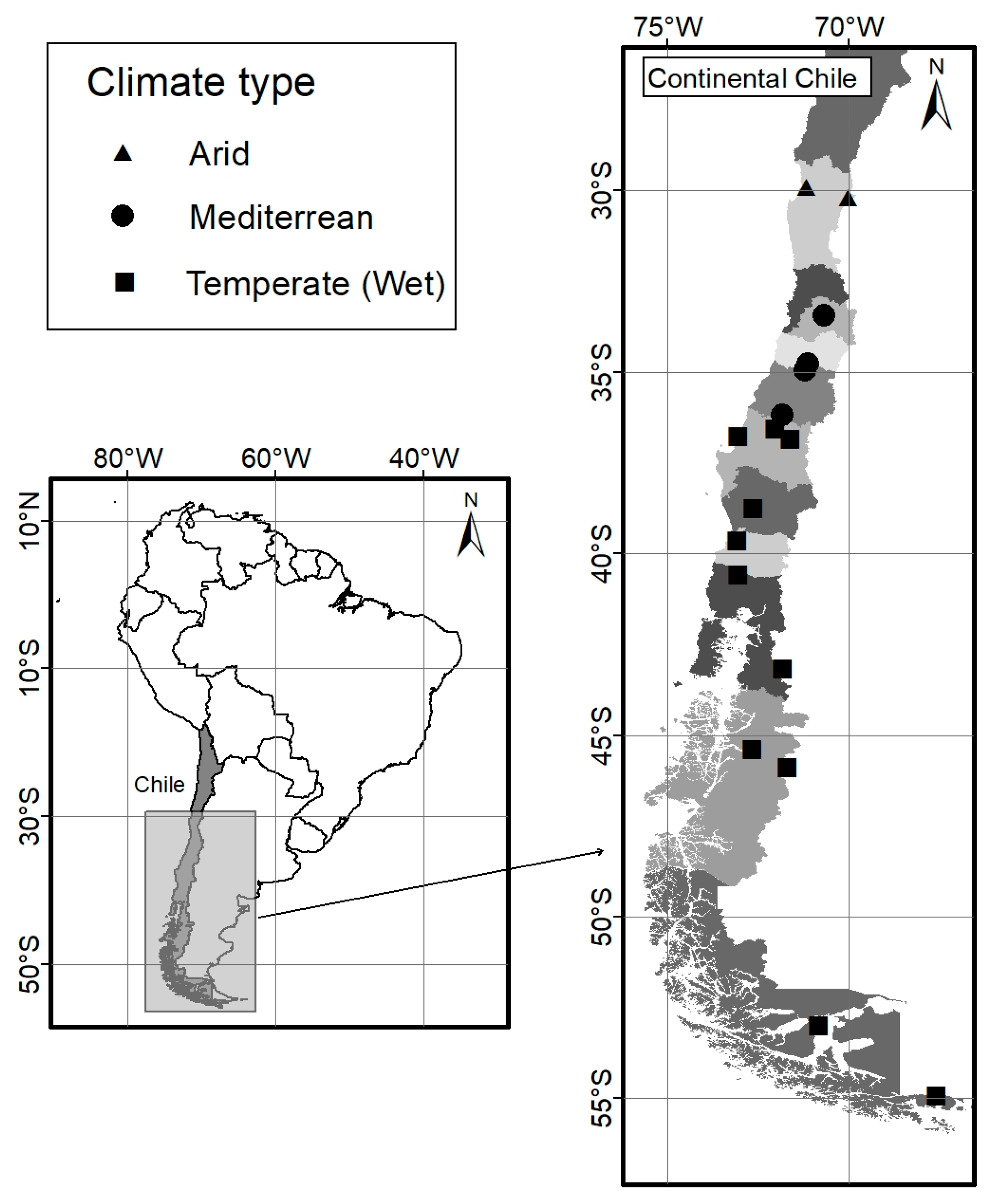
2.1. Meteorological Stations and Climatic Data

Latitude is the main variable that explains precipitation variations in Chile (i.e., for the most part of the country precipitation increases with latitude). Climatic zones also change with elevation and proximity to the ocean. Annual temperature variations are smaller in coastal cities, resulting in milder winters and summers. On the other hand, precipitation tends to increase near the Andes mountain range [48].

Figure 2 and

Table 1. General characteristics of the rainfall stations used in this study.

Station Name	Climate	Latitude (° South)	Longitude (° West)	Elevation (m a.s.l.)	Begginning	End	% Missing Data	Average Annual Precipitation (mm)
La Serena	Arid	29°55′	71°12′	142	01/01/1950	31/12/2013	3.6	84.3
Embalse La Laguna	Arid	30°12′	70°02′	3160	01/01/1964	31/12/2013	0.7	159.7
Santiago	Mediterrean	33°27′	70°40′	527	01/01/1950	31/12/2013	0	314.1
Rancagua	Mediterrean	34°46′	71°07′	239	01/09/1971	31/12/2013	1.5	691.7
Curicó	Mediterrean	34°58′	71°13′	225	01/01/1950	31/12/2013	10.4	675,5
Parral	Temperate	36°11′	71°49′	175	01/02/1993	31/12/2013	0	952.2
Diguillin	Temperate	36°52′	71°38′	670	01/05/1959	31/12/2013	0.8	2091.5
Chillán	Temperate	36°35′	72°02′	151	01/01/1950	31/12/2013	12.6	1044.0
Concepción	Temperate	36°46′	73°03′	12	01/01/1950	31/12/2013	0	1119.5
Temuco	Temperate	38°46′	72°38′	92	01/01/1950	31/12/2013	13.0	1163.4
Futaleufu	Temperate	43°11′	71°51′	350	01/01/1960	31/12/2013	2.7	2133.8
Osorno	Temperate	40°36′	73°03′	61	01/01/1950	31/12/2013	10.8	1358.1
Balmaceda	Temperate	45°54′	71°41′	520	01/01/1958	31/12/2013	0	576.3
Puerto Aysén	Temperate	45°24′	72°42′	10	01/01/1950	31/12/2013	7.9	2661.6
Punta Arenas	Temperate	53°00′	70°50′	39	01/01/1950	31/12/2013	3.2	399.7
Puerto Williams	Temperate	54°55′	67°37′	30	01/01/1950	31/12/2013	19.9	480.8
Valdivia	Temperate	39°39′	73°04′	18	01/01/1950	31/12/2013	3.7	1836.2

present the selected 17 rain gauges and their main characteristics. The stations were distributed between latitudes 29°55′12′′ S and 59°93′40′′ S, and were part of two national rain gauge networks managed by the Dirección General de Aguas (DGA) and the Dirección Meteorológica de Chile (DMC). Daily precipitation records have a duration ranging from 21 years (1 gauge) to 64 years (11 gauges). The time series of the monthly observed sea surface temperature anomalies in the Niño region 3.4 (ENSO index) was obtained from the National Oceanic and Atmospheric Administration (NOAA (2017) [49]).

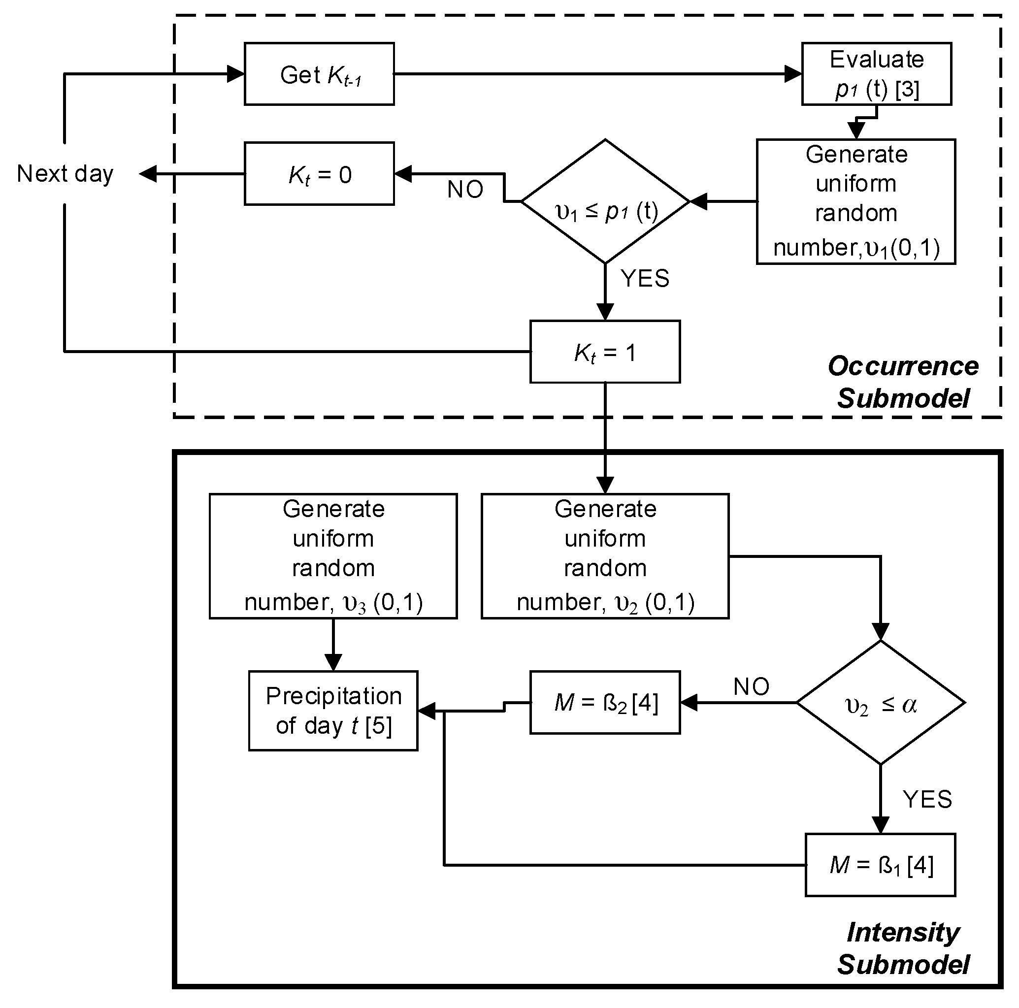
2.2. Precipitation Occurrence Submodel

Precipitation occurrence was modeled as a two-stage, first-order Markov chain. Hence, the conditional probability of precipitation occurrence on a specific day depends only on the precipitation occurrence in the previous one. The occurrence of precipitation in day t is treated as a binary variable K_t with value 1 or 0, in case of non-zero or no precipitation, respectively. The first-order Markov chain model is characterized by the transition probabilities $p_{01}$ (i.e., probability of having a rainy day after a dry day), and $p_{11}$ (i.e., probability of having a rainy day following a rainy day):

$$p_{01} \left(t\right)=Pr(K_t=1 |K_{t-1}=0).$$

(1)

$$p_{11} \left(t\right)=Pr(K_t=1 |K_{t-1}=1).$$

(2)

where Pr denotes probability. The model used to represent precipitation occurrence is a binomial GLM. Note that the expected value of a binomial distribution with a single trial (also called a Bernoulli distribution) is the underlying success probability, i.e., the unconditional probability of having rain the day t ($p_1\left(t\right)$) in our case. Thus, a binomial GLM with a logistic function was used to link the covariables to precipitation occurrence. The primary covariable is the occurrence of rainfall on the previous day K_t−1, while the ENSO index is the second covariable. In this way, the conditional probabilities of the first-order Markov chain are being considered. Additional covariables, such as a seasonal cycle or other climatic indices, could be included if needed. The following expression was used to obtain $p_1\left(t\right)$.

$$p_1 \left(t\right) =\frac{\exp \left[C_0+C_1{K}_{t-1}+C_2\mathrm{ENSOindex}\right]}{1+\exp \left[C_0+C_1{K}_{t-1}+C_2\mathrm{ENSOindex}\right]}$$

(3)

Here $C_0$ corresponds to the intercept, $C_1$ is the associated parameter of $K_{t-1}$, and $C_2$ the coefficient that describes the influence of the ENSO index.

Given the strong seasonality of the precipitation regime, the parameters of the model used to estimate $p_1 \left(t\right)$ were fitted individually to each month, using the maximum likelihood approach with a numerical optimization procedure. The same approach has been followed by other authors (see as examples Furrer and Katz [50] and Wilks [51]).To determine whether precipitation occurs in the simulated day, a uniform random number (υ₁) is generated. If $p_1\left(t\right)$ ≤ υ₁ a rainfall event is simulated, otherwise the day is considered to be dry (Figure 3).

2.3. Precipitation Intensity Submodel

Precipitation is usually associated to frontal systems with rather intensive values, but sometimes small rain events occur. In order to account for both types in a single model, a mixed exponential distribution function with parameters α, ${\mathrm{ß}}_1$, and ${\mathrm{ß}}_2$ was used:

$$f\left(x\right)=\frac{\alpha }{{\mathrm{ß}}_1}{\exp }^{[\raisebox{1ex}{$-x$}\!\left/ \!\raisebox{-1ex}{${\text{ß}}_1]$}\right.}+\frac{1-\alpha }{{\mathrm{ß}}_2}{\exp }^{[\raisebox{1ex}{$-x$}\!\left/ \!\raisebox{-1ex}{${\text{ß}}_2]$}\right.}$$

(4)

This model was used for any day t when $K_t=1$. The parameter α represents the probability of having a precipitation intensity from one of the specific exponential distribution within the mixed function. Thus, if α is larger than a random uniform number υ₂ between 0 and 1, then the precipitation follows an exponential distribution with mean M = ${\mathrm{ß}}_1$, otherwise M = ${\mathrm{ß}}_2$. Note that ${\mathrm{ß}}_1$ and ${\mathrm{ß}}_2$ correspond to magnitudes thar are low and high respectively. Finally, the precipitation of day t (P_t) is obtained as:

$$P_t=-\ln (1-{\upsilon }_3)M$$

(5)

where ${\upsilon }_3$ is a random uniform number between 0 and 1. Because of the seasonality in precipitation, parameters α, ${\mathrm{ß}}_1$, ${\mathrm{ß}}_2$ are estimated monthly using the maximum likelihood approach (Figure 3).

3. Results

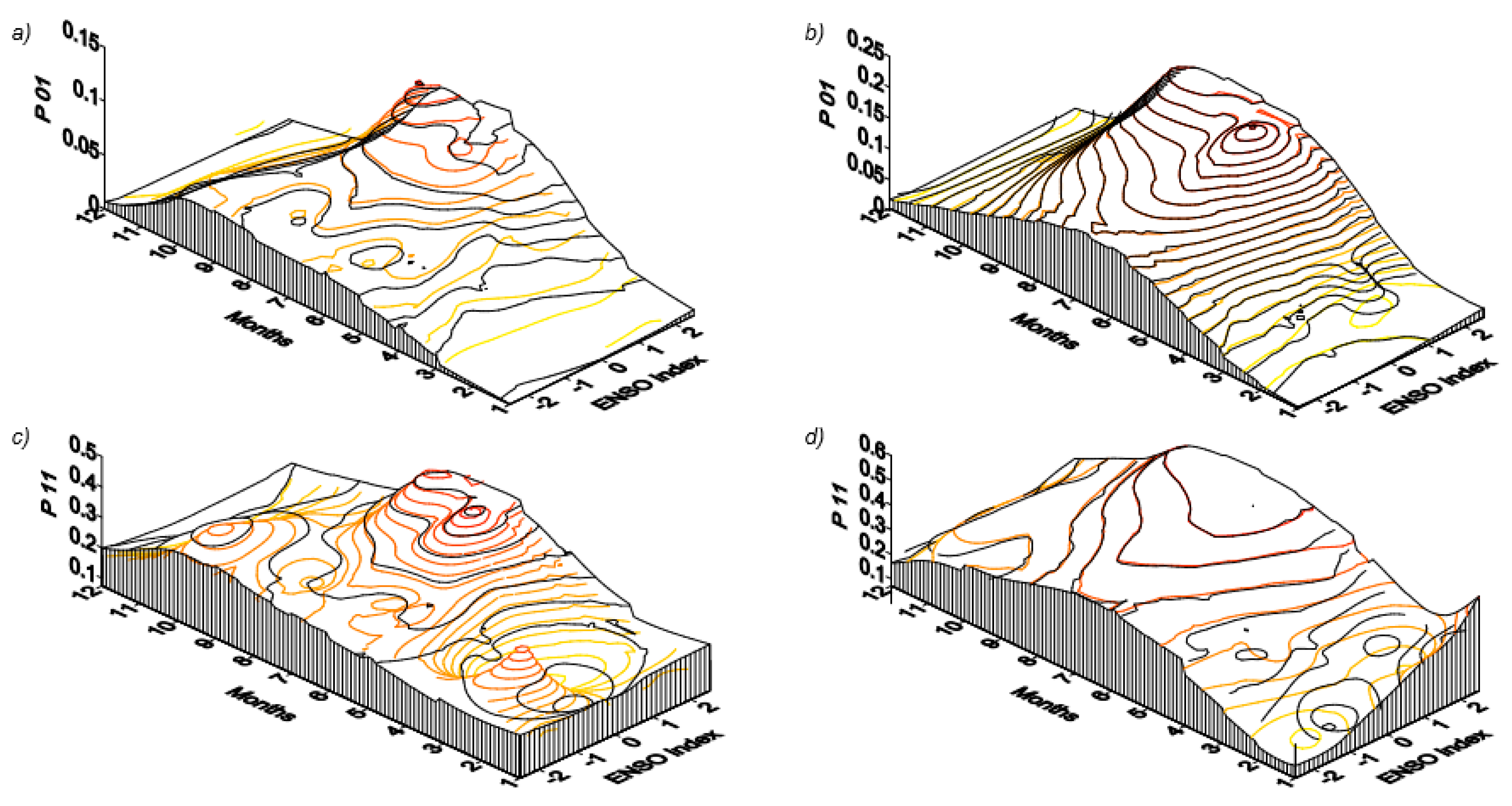
3.1. Precipitation Occurrence

Table 2. Parameters of the generalized lineal model (GLM) (Equation (3)) for August, considering precipitation occurrence in the previous day (K_t−1) and the El Niño-Southern Oscillation (ENSO) index as a covariable. Bold values denote statistical significance (p value < 0.05) in the parameters.

Station Name	GLM Parameters			Goodness of Fit with ENSO Index			Goodness of Fit without ENSO Index
	${\mathit{C}}_0$	${\mathit{C}}_1$	${\mathit{C}}_2$	R2	RMSE	AIC	R2	RMSE	AIC
La Serena	−2.80	1.81	0.40	0.70	0.10	890.90	0.51	0.70	966.91
Embalse La Laguna	−3.11	2.45	0.40	0.62	0.61	645.22	0.43	2.31	670.46
Santiago	−1.83	1.64	0.10	0.56	0.94	1800.51	0.33	3.10	2100.67
Rancagua	−1.71	1.72	0.10	0.76	0.91	1277.10	0.52	4.58	1877.21
Curicó	−1.43	1.43	0.20	0.48	0.70	1744.11	0.34	0.91	1750.84
Parral	−1.15	1.32	0.05	0.67	0.97	1863.85	0.53	1.19	1975.91
Diguillin	−1.03	1.51	0.08	0.42	1.15	2044.91	0.47	1	2043.22
Chillán	−1.10	1.42	0.10	0.53	1	2060.73	0.53	1	2061.11
Concepción	−0.92	1.51	0.01	0.33	1.10	2434.81	0.30	1.16	2436.80
Temuco	−0.53	1.41	−0.07	0.52	1.12	2119.91	0.41	1.17	2125.91
Futaleufu	−0.45	1.43	−0.09	0.22	1.18	1934.75	0.20	1.19	1934.69
Osorno	−0.40	1.51	−0.01	0.43	1.09	2112.81	0.43	1.11	2114.88
Balmaceda	−0.81	1.15	−0.01	0.52	1.32	2226.31	0.50	1.21	2228.39
Puerto Aysén	0.10	1.51	−0.10	0.64	1.05	2058.81	0.62	1.06	2057.61
Punta Arenas	−0.91	0.83	0.09	0.42	1.05	2315.61	0.40	1.10	2416.10
Puerto Williams	−1.01	0.92	−0.12	0.33	1	1900.11	0.21	1.12	1955.41
Valdivia	−0.33	1.71	−0.01	0.34	1.06	2146.54	0.32	1	2100.62

compares the coefficients C₀, C₁, and C₂ of the GLM model for precipitation occurrence including ENSO (values of the coefficients for the model that do not incorporate this covariable are not shown), and the basic goodness of fit statistics (i.e., coefficient of determination (R²), Akaike information criterion (AIC) [52], and the root mean square error (RMSE)) for both models. This comparison is shown for August, although similar results were obtained for the autumn and winter seasons. Incorporating the ENSO index improves the estimation of the precipitation occurrence during these months, mostly in arid and Mediterranean areas. For example, the La Serena rain gauge R² increased from 0.5 to 0.7, and the AIC decreased from 966.9 to 890.9 in August, once the ENSO index was added to the GLM model only based on K_t-1.

Figure 4 compares the observed and simulated conditional probabilities $p_{01}$ and $p_{11}$ for the stations in La Serena and Santiago. The probability $p_{11}$ is larger than $p_{01}$, reflecting the degree of persistence in the precipitation process, as the lag one autocorrelation corresponds to the difference between $p_{11}$ and $p_{01}$. The probability $p_{01}$ ranges from 0.01 to 0.15 in La Serena (Figure 4a) and from 0 to 0.25 in Santiago (Figure 4b). The probability $p_{11}$ ranges from 0.06 to 0.5 in La Serena (Figure 4c) and from 0.05 to 0.6 in Santiago (Figure 4d).

In both locations, the ENSO index influences the precipitation occurrence. Specifically, when this covariable has values between 0.5 and 2.5 (i.e., during warmer than normal conditions known as El Niño), the probability of precipitation occurrence increases with the ENSO index. Conversely, during La Niña, the probability of precipitation occurrence decreases with the ENSO index, regardless of the dry or wet condition of the previous day. Interestingly, the contours of the historical and simulated probabilities behave similarly, as the GLM model is able to reproduce the seasonality of the probabilities, which are larger for the winter months (June, July, and August) and smaller during the summer months (December, January, and February).

Table 3. Contingency table of daily frequencies of dry and wet days from observations and simulations obtained from 10 random years.

Climate Type	Station Name	Observed	GLM with ENSO Index		HSS	GLM without ENSO Index		HSS
			(0)	(1)		(0)	(1)
Arid	La Serena	(0)	3340	95	0.52	3303	132	0.01
		(1)	100	118		208	10
Arid	Embalse La Laguna	(0)	3320	119	0.46	3318	121	0.03
		(1)	105	109		201	13
Mediterrean	Santiago	(0)	3000	272	0.16	2956	316	0.04
		(1)	290	90		330	50
Mediterrean	Rancagua	(0)	2756	350	0.12	2744	367	0.10
		(1)	421	120		423	118
Mediterrean	Curicó	(0)	2621	430	0.13	2631	420	0.11
		(1)	441	161		452	150
Temperate	Parral	(0)	2306	573	0.12	2365	514	0.11
		(1)	523	250		551	222
Temperate	Diguillin	(0)	2212	586	0.12	2130	668	0.09
		(1)	574	281		573	282
Temperate	Chillán	(0)	2194	556	0.15	2183	567	0.13
		(1)	590	312		599	303
Temperate	Concepción	(0)	2054	638	0.13	1995	661	0.10
		(1)	632	364		649	347
Temperate	Temuco	(0)	1411	756	0.10	1403	773	0.09
		(1)	821	655		818	658
Temperate	Futaleufu	(0)	1100	849	0.09	1100	849	0.04
		(1)	900	804		900	804
Temperate	Osorno	(0)	1096	806	0.09	1133	769	0.08
		(1)	859	891		902	848
Temperate	Balmaceda	(0)	1640	777	0.05	1663	754	0.01
		(1)	780	456		844	392
Temperate	Puerto Aysén	(0)	1008	766	0.04	1025	709	0.02
		(1)	1000	878		1090	828
Temperate	Punta Arenas	(0)	1973	618	0.22	2004	73	0
		(1)	1500	61		1516	59
Temperate	Puerto Williams	(0)	1008	726	0.04	1025	709	0.02
		(1)	1040	878		1090	828
Temperate	Valdivia	(0)	898	629	0.09	898	629	0.07
		(1)	1043	1082		1087	1038

summarizes the contingency tables for the number of observed and simulated rainy and dry days, considering 10 random years. Again, the GLM model performs better when the ENSO index is included, for both rainy and dry days, particularly in arid and Mediterranean climates. We used the Heidke skill score (HSS) [53] to assess the overall performance of the model. Negative HSS values indicate that a random forecast is better, 0 means no skill, and 1 means perfect forecast. There is a significant improvement in this score when using the ENSO index for gauges in an arid climate.

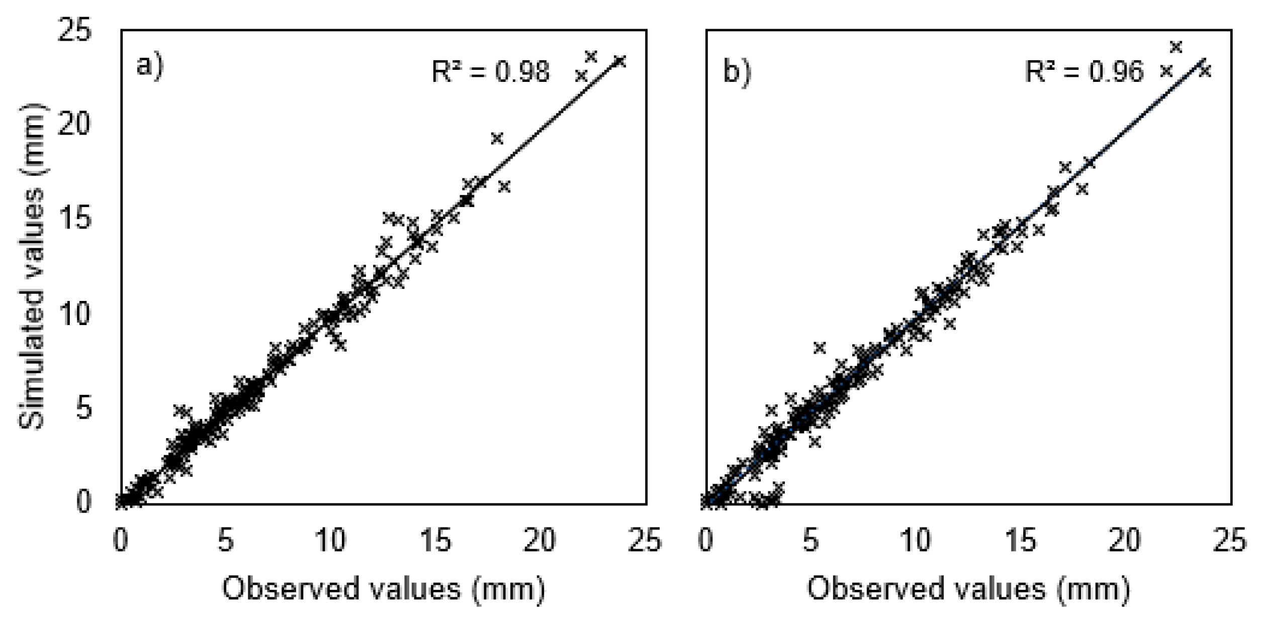
3.2. Precipitation Intensity

3.2.1. Annual Precipitation

The model is now evaluated in terms of its capability to reproduce annual precipitation. Figure 5 shows the relative difference (%) between observed and synthetically simulated average values of this variable. This difference varies among the climates, and tends to be larger for the gauges located in arid regions. In fact, there is an error of ~9% for La Serena gauge (i.e., the observed and simulated annual average are 84.3 and 76.8 mm respectively). Overall, larger errors in arid regions with long dry periods are partially explained by the larger number of zero precipitation days through the year, which affects the estimation of the model’s parameters. Nevertheless, annual precipitation totals and standard deviations for all of the Chilean stations are simulated reasonably well, as illustrated in Figure 6.

3.2.2. Monthly Precipitation

Figure 7 shows a box-plot diagram comparing synthetically generated and historical monthly precipitation grouped for the spring–summer and autumn–winter months for La Serena and Balmaceda. Similarly, Figure 8 presents the same results for Santiago and Puerto Aysén. Similar results to those presented in Figure 7c,d and Figure 8c,d were found for the remaining temperature stations. Overall, monthly precipitation in winter was better estimated, for both the temperate and Mediterranean climates. However, for the La Serena gauge (arid climate), the model generated precipitation values different than the historical ones during spring and summer months. For example, in February the 25th percentile, or quartile Q₃, of the synthetically generated values is the same as the maximum historical precipitation (Figure 7a). This difference is explained by the fact that a few precipitation outliers affected the distribution of synthetically generated data in that month. On the other hand, the model is able to generate monthly precipitation values similar to the observed ones for autumn and winter months, as shown in Figure 8b,d. In Santiago, the minimum and maximum observed daily precipitation values in July were 0.2 mm and 27.1 mm, while the simulated ones were 0.5 mm and 27 mm. Similarly, the observed 75th, 50th, and 25th percentiles (i.e., quartiles Q₁, Q₂, and Q₃) are 12.0 mm, 2.9 mm, and 0.9 mm, values that compare very well with the simulated ones, which are 11.9 mm, 3.2 mm, and 0.7, mm (Figure 8b).

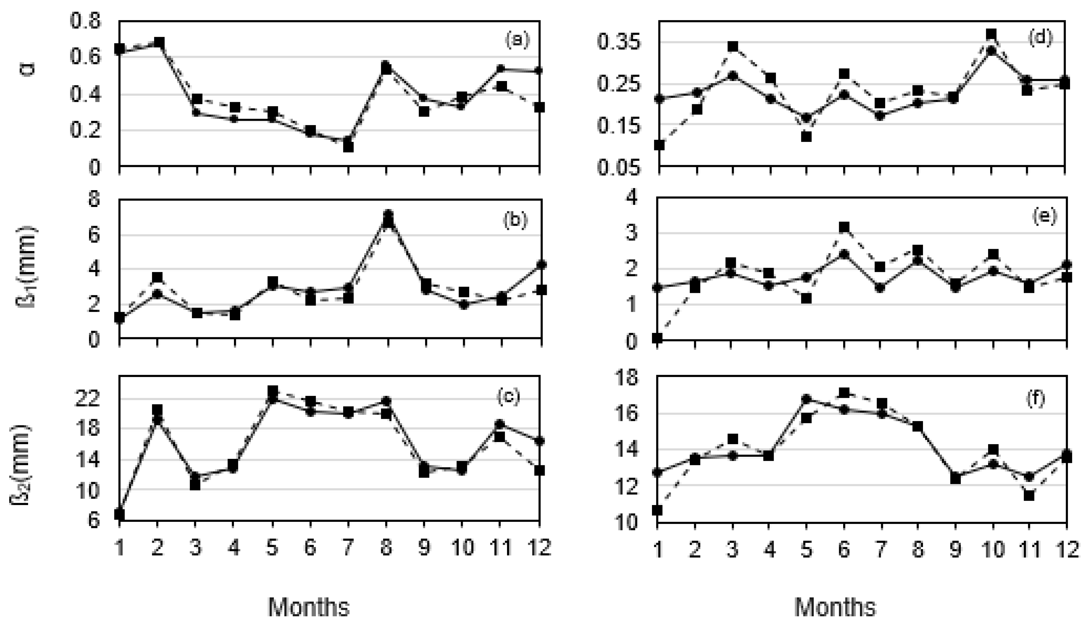
3.2.3. Mixed Exponential Distribution Parameters

Figure 9 compares the values of parameters α, ${\mathrm{ß}}_1$, and ${\mathrm{ß}}_2$ used in the mixed exponential distribution for both observed and simulated series. Overall, monthly values of α for Rancagua located in the Mediterranean climate (Figure 9a) were similar, with the largest differences taking place in December (i.e., 0.5 for the historical data, vs. 0.31 for the synthetically generated data). In winter months, values of α close to zero imply that a unique distribution with parameter ${\mathrm{ß}}_2$ will suffice to represent the phenomenon. On the other hand, α values were closer to 1 for dry months, and thus the simulated precipitation is drawn from a distribution with a single parameter ${\mathrm{ß}}_1$. Parameters ${\mathrm{ß}}_1$ and ${\mathrm{ß}}_2$ obtained from synthetically generated data for La Serena were very close to the observed ones, and properly represented the seasonality of the record (Figure 9b,c). In the case of the Puerto Aysén gauge (temperate climate), more differences were observed for parameter α, particularly in January, March, April, May, June (Figure 9d). Again, parameters ${\mathrm{ß}}_1$ and ${\mathrm{ß}}_2$ from the synthetically generated data and from the records were alike, although some differences correlated with differences in α, are observed through the year (Figure 9e,f).

3.2.4. Interannual Variability

Figure 10 compares the standard deviation for monthly precipitation amounts calculated from the observed and simulated data, both with and without the ENSO index as a covariable. The results for all stations and for all twelve calendar months have been combined, in order to have an overall assessment of the ability of the model to simulate interannual variability. The GLM model with one variable (K_t−1) underestimated the interannual variability, particularly during those months with less precipitation in arid and Mediterrenean climates. In contrast, the standard deviation values were better represented when incorporating the ENSO index, which implies an improvement in the simulation of the interannual variability. Standard deviations of the number of wet days from the observations, and those from simulations conducted with and without the ENSO index models, are given in Figure 11. Using the ENSO index as a covariate improved the representation of the interannual variability of the frequency of wet days. This indicates that the overdispersion problem in the model for monthly precipitation totals is the result of its inability to produce a sufficiently large variance in the number of wet days.

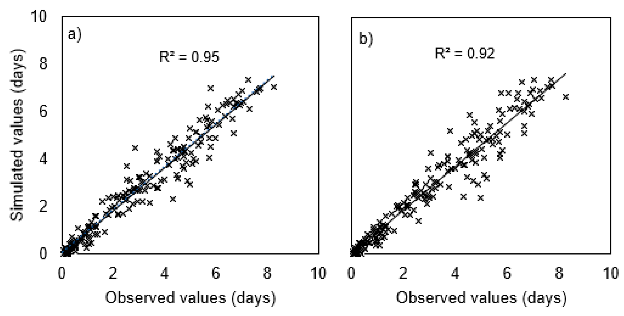
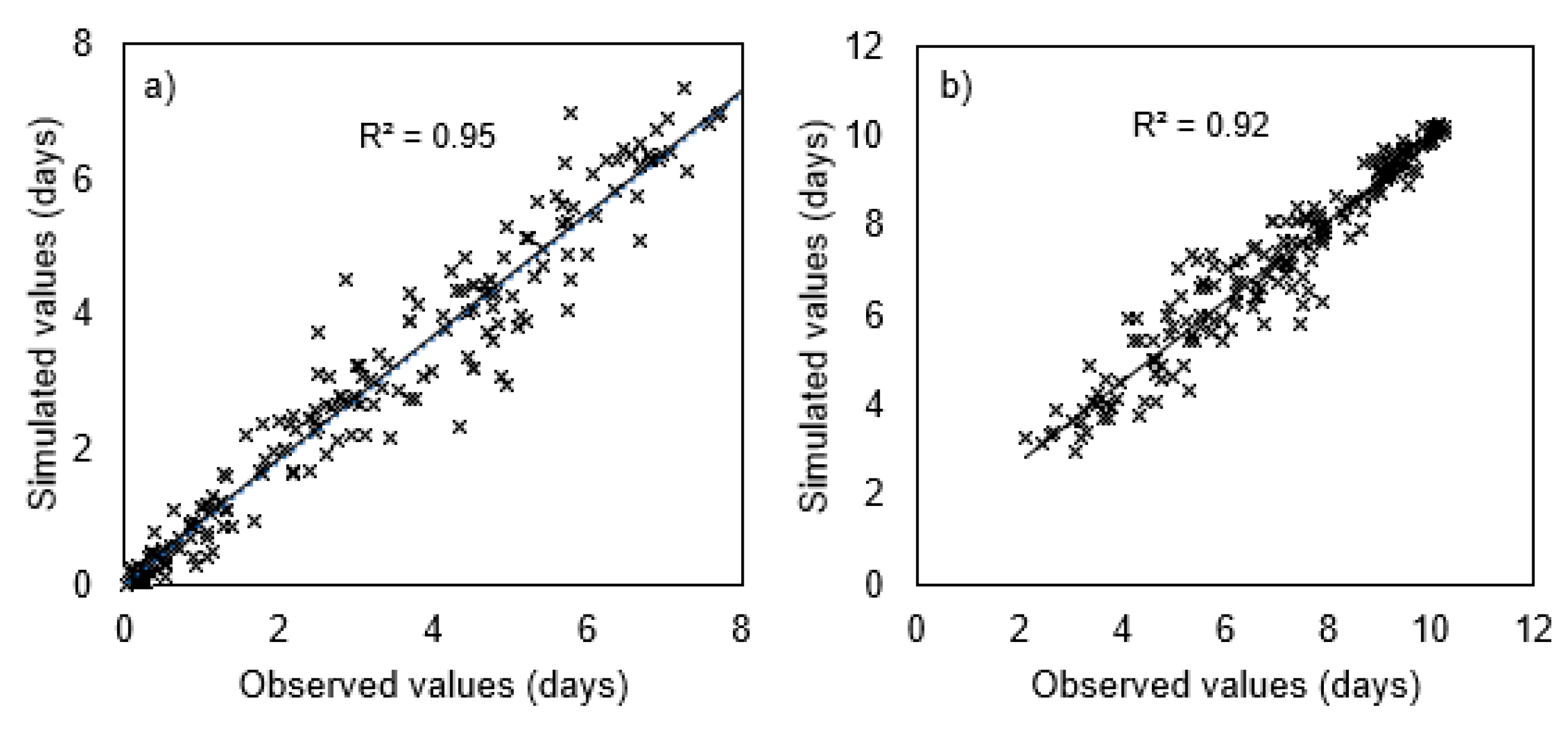
3.2.5. Wet and Dry Spell Durations

The average observed and simulated length of wet and dry spells for all seasons are compared in Figure 12. Simulations were carried out using the ENSO index model. Considering the ENSO index produced slightly longer dry and wet spells, indicating that wet spells length tends to be underestimated by the model, particularly for long durations. On the other hand, the length of dry spells tended to be overestimated by the model for short durations.

4. Discussion and Conclusions

This study shows that incorporating the ENSO index as a covariable in a GLM scheme improves the representation of the precipitation occurrence process (i.e., it allows a better estimation of transition probabilities) in the arid and Mediterranean zones of Chile. This situation was introduced by Furrer and Katz [37,50] for an Argentinean area, located at a latitude similar that to Santiago. In addition, Montecinos and Aceituno [44] indicate that during episodes of El Niño there is a tendency to increase the average precipitation during winter, between 30° and 35° S, and during late spring, between 35° and 38° S (Mediterranean), mostly because of an increase in the frequency of rainy days rather than an increase in the daily magnitude. On the other hand, the ENSO index does not significantly contribute to the estimation of precipitation occurrence in the temperate regions of Chile (i.e., Valdivia and Puerto Aysén). We found that the ENSO index produces the same effect of on both $p_{01}$ and $p_{11}$: higher positive ENSO index values induce a greater probability of rainfall, irrespective of whether the previous day was wet or dry. Hence, the model is able to increase the frequency of rain during an El Niño phase, and decrease it during La Niña events.

Our results are in agreement with the findings of Breinl et al. [54] who used a semi-parametric WG, and demonstrated that simulations are less biased in wet temperate climates than in dry climates. Nevertheless, the error in the estimation of average annual precipitation in the arid regions of Chile associated with the model proposed (i.e., 8.94%) is much less than that obtained by Taulis and Milke [31], who overestimated the average annual precipitation in the same region by 42% when using gamma distribution for daily precipitation (WGEN). Also, our results confirm the arguments of Li et al. [55], who suggested that functions with more parameters improve the estimates of daily rainfall. In particular, using the mixed exponential distribution allows for a better reproduction the interannual variability [56]. Nevertheless, caution must be taken when using more parameters, in order to avoid the potential issue of overfitting, which can limit the applicability to additional data.

Although arid, Mediterranean, and temperate climates are the focus of the study, these results are in agreement with those from studies developed in other climate zones. For example, Wilby et al. [57] found that the covariable North Atlantic Oscillation (NAO) index and area average sea surface temperature (SST) anomalies can explain the precipitation occurrence for different weather seasons across the British Isles. Hence, this study can be added to a growing body of literature focused on understanding and incorporating global phenomena in the ocean–atmosphere system during the development of WGs.

References

1. Richardson, C.W.; Wright, D.A. WGEN: A Model for Generating Daily Weather Variables; U.S. Department of Agriculture, Agricultural Research Service: Washington, DC, USA, 1984.
2. Ebrahimpour, M.; Ghahreman, N.; Orang, M. Assessment of climate change impacts on reference evapotranspiration and simulation of daily weather data using SIMETAW. J. Irrig. Drain. Eng. 2013, 140, 04013012. [Google Scholar] [CrossRef]
3. Graae, B.J.; De Frenne, P.; Kolb, A.; Brunet, J.; Chabrerie, O.; Verheyen, K.; Pepin, N.; Heinken, T.; Zobel, M.; Shevtsova, A. On the use of weather data in ecological studies along altitudinal and latitudinal gradients. Oikos 2012, 121, 3–19. [Google Scholar] [CrossRef]
4. Gleason, M.L.; Duttweiler, K.B.; Batzer, J.C.; Taylor, S.E.; Sentelhas, P.C.; Monteiro, J.E.B.A.; Gillespie, T.J. Obtaining weather data for input to crop disease-warning systems: Leaf wetness duration as a case study. Sci. Agric. 2008, 65, 76–87. [Google Scholar] [CrossRef]
5. Strandman, H.; Väisänen, H.; Kellomäki, S. A procedure for generating synthetic weather records in conjunction of climatic scenario for modelling of ecological impacts of changing climate in boreal conditions. Ecol. Model. 1993, 70, 195–220. [Google Scholar] [CrossRef]
6. Wilks, D.S.; Wilby, R.L. The weather generation game: A review of stochastic weather models. Prog. Phys. Geogr. 1999, 23, 329–357. [Google Scholar] [CrossRef]
7. Richardson, C.W. Stochastic simulation of daily precipitation, temperature, and solar radiation. Water Resour. Res. 1981, 17, 182–190. [Google Scholar] [CrossRef]
8. Sharpley, A.N.; Williams, J.R. EPIC-Erosin/Productivity Impact Calculator: 1. Model Documentation; USDA: Washington, DC, USA, 1990.
9. Nicks, A.D.; Lane, L.J.; Gander, G.A. Weather Generator. In USDA-Water Erosion Prediction Project: Hillslope Profile Model Documentation; Report; NSERL: West Lafayette, IN, USA, 1995. [Google Scholar]
10. Lobo, G.P.; Frankenberger, J.R.; Flanagan, D.C.; Bonilla, C.A. Evaluation and improvement of the CLIGEN model for storm and rainfall erosivity generation in Central Chile. Catena 2015, 127, 206–213. [Google Scholar] [CrossRef]
11. Racsko, P.; Szeidl, L.; Semenov, M. A serial approach to local stochastic weather models. Ecol. Model. 1991, 57, 27–41. [Google Scholar] [CrossRef]
12. Semenov, M.A.; Barrow, E.M. Use of a stochastic weather generator in the development of climate change scenarios. Clim. Chang. 1997, 35, 397–414. [Google Scholar] [CrossRef]
13. Semenov, M.A.; Barrow, E.M. LARS-WG: A Stochastic Weather Generator for Use in Climate Impact Studies. 2002. Available online: http://resources.rothamsted.ac.uk/sites/default/files/groups/mas-models/download/LARS-WG-Manual.pdf (accessed on 1 February 2018).
14. McKague, K.; Rudra, R.; Ogilvie, J. CLIMGEN-A Convenient Weather Generation tool for Canadian Climate Stations. In Proceedings of the Meeting of the CSAE/SCGR Canadian Society for Engineering in Agricultural Food and Biological Systems, Montreal, QC, Canada, 6–9 July 2003; pp. 6–9. [Google Scholar]
15. Chen, J.; Brissette, F.P.; Leconte, R. A daily stochastic weather generator for preserving low-frequency of climate variability. J. Hydrol. 2010, 388, 480–490. [Google Scholar] [CrossRef]
16. Chen, J.; Brissette, F.P.; Leconte, R. WeaGETS—A Matlab-based daily scale weather generator for generating precipitation and temperature. Procedia Environ. Sci. 2012, 13, 2222–2235. [Google Scholar] [CrossRef]
17. Dubrovský, M.; Buchtele, J.; Žalud, Z. High-frequency and low-frequency variability in stochastic daily weather generator and its effect on agricultural and hydrologic modelling. Clim. Chang. 2004, 63, 145–179. [Google Scholar] [CrossRef]
18. Wetterhall, F.; Bárdossy, A.; Chen, D.; Halldin, S.; Xu, C. Statistical downscaling of daily precipitation over Sweden using GCM output. Theor. Appl. Climatol. 2009, 96, 95. [Google Scholar] [CrossRef]
19. Bardossy, A.; Plate, E.J. Space-time model for daily rainfall using atmospheric circulation patterns. Water Resour. Res. 1992, 28, 1247–1259. [Google Scholar] [CrossRef]
20. Pickering, N.B.; Hansen, J.W.; Jones, J.W.; Wells, C.M.; Chan, V.K.; Godwin, D.C. WeatherMan: A utility for managing and generating daily weather data. Agron. J. 1994, 86, 332–337. [Google Scholar] [CrossRef]
21. Jones, P.G.; Thornton, P.K. MarkSim: Software to generate daily weather data for Latin America and Africa. Agron. J. 2000, 92, 445–453. [Google Scholar] [CrossRef]
22. Qian, B.; Gameda, S.; Hayhoe, H.; De Jong, R.; Bootsma, A. Comparison of LARS-WG and AAFC-WG stochastic weather generators for diverse Canadian climates. Clim. Res. 2004, 26, 175–191. [Google Scholar] [CrossRef]
23. Qian, B.; Gameda, S.; Hayhoe, H. Performance of stochastic weather generators LARS-WG and AAFC-WG for reproducing daily extremes of diverse Canadian climates. Clim. Res. 2008, 37, 17–33. [Google Scholar] [CrossRef]
24. Mavromatis, T.; Hansen, J.W. Interannual variability characteristics and simulated crop response of four stochastic weather generators. Agric. For. Meteorol. 2001, 109, 283–296. [Google Scholar] [CrossRef]
25. Gaur, A.; Simonovic, S.P. Towards reducing climate change impact assessment process uncertainty. Environ. Process. 2015, 2, 275–290. [Google Scholar] [CrossRef]
26. King, L.M.; McLeod, A.I.; Simonovic, S.P. Simulation of historical temperatures using a multi-site, multivariate block resampling algorithm with perturbation. Hydrol. Process. 2014, 28, 905–912. [Google Scholar] [CrossRef]
27. King, L.M.; McLeod, A.I.; Simonovic, S.P. Improved weather generator algorithm for multisite simulation of precipitation and temperature. J. Am. Water Resour. Assoc. 2015, 51, 1305–1320. [Google Scholar] [CrossRef]
28. Jones, P.D.; Kilsby, C.G.; Harpham, C.; Glenis, V.; Burton, A. UK Climate Projections Science Report: Projections of Future Daily Climate for the UK from the Weather Generator; University of Newcastle: Newcastle, UK, 2009. [Google Scholar]
29. Christierson, B.V.; Vidal, J.-P.; Wade, S.D. Using UKCP09 probabilistic climate information for UK water resource planning. J. Hydrol. 2012, 424, 48–67. [Google Scholar] [CrossRef]
30. Wan, H.; Zhang, X.; Barrow, E.M. Stochastic modelling of daily precipitation for Canada. Atmos. Ocean 2005, 43, 23–32. [Google Scholar] [CrossRef]
31. Taulis, M.E.; Milke, M.W. Estimation of WGEN weather generation parameters in arid climates. Ecol. Model. 2005, 184, 177–191. [Google Scholar] [CrossRef] [Green Version]
32. Wilks, D.S. Extending logistic regression to provide full-probability-distribution MOS forecasts. Meteorol. Appl. 2009, 16, 361–368. [Google Scholar] [CrossRef]
33. Stern, R.D.; Coe, R. A model fitting analysis of daily rainfall data. J. R. Stat. Soc. Ser. A Gen. 1984, 147, 1–34. [Google Scholar] [CrossRef]
34. Yang, C.; Chandler, R.E.; Isham, V.S.; Wheater, H.S. Spatial-temporal rainfall simulation using generalized linear models. Water Resour. Res. 2005, 41. [Google Scholar] [CrossRef]
35. Chandler, R.E. On the use of generalized linear models for interpreting climate variability. Environmetrics 2005, 16, 699–715. [Google Scholar] [CrossRef]
36. Verdin, A.; Rajagopalan, B.; Kleiber, W.; Katz, R.W. Coupled stochastic weather generation using spatial and generalized linear models. Stoch. Environ. Res. Risk Assess. 2015, 29, 347–356. [Google Scholar] [CrossRef]
37. Furrer, E.M.; Katz, R.W. Improving the simulation of extreme precipitation events by stochastic weather generators. Water Resour. Res. 2008, 44, 76. [Google Scholar] [CrossRef]
38. Kim, Y.; Katz, R.W.; Rajagopalan, B.; Podestá, G.P.; Furrer, E.M. Reducing overdispersion in stochastic weather generators using a generalized linear modeling approach. Clim. Res. 2012, 53, 13–24. [Google Scholar] [CrossRef]
39. Katz, R.W.; Parlange, M.B. Overdispersion phenomenon in stochastic modeling of precipitation. J. Clim. 1998, 11, 591–601. [Google Scholar] [CrossRef]
40. Walker, G.T. Correlations in seasonal variations of weather. I. A further study of world weather. Mem. Indian Meteorol. Dep. 1924, 24, 275–332. [Google Scholar] [CrossRef]
41. Ropelewski, C.F.; Halpert, M.S. Quantifying southern oscillation-precipitation relationships. J. Clim. 1996, 9, 1043–1059. [Google Scholar] [CrossRef]
42. Kane, R.P. Rainfall extremes in some selected parts of Central and South America: ENSO and other relationships reexamined. Int. J. Climatol. 1999, 19, 423–455. [Google Scholar] [CrossRef]
43. Meza, F.J. Recent trends and ENSO influence on droughts in Northern Chile: An application of the Standardized Precipitation Evapotranspiration Index. Weather Clim. Extremes 2013, 1, 51–58. [Google Scholar] [CrossRef]
44. Montecinos, A.; Aceituno, P. Seasonality of the ENSO-related rainfall variability in central Chile and associated circulation anomalies. J. Clim. 2003, 16, 281–296. [Google Scholar] [CrossRef]
45. Aceituno, P.; Fuenzalida, H.; Rosenblüth, B. Climate along the extratropical west coast of South America. In Earth Systems Responses Global Change; Mooney, H.A., Fuentes, E.R., Kronb, B.I., Eds.; Academic Press: San Diego, CA, USA, 1993; pp. 61–69. [Google Scholar]
46. Quintana, J.; Aceituno, P. Trends and interdecadal variability of rainfall in Chile. In Proceedings of the 8 ICSHMO, Foz do Iguacu, Brazil, 24–28 April 2006; pp. 24–28. [Google Scholar]
47. Masiokas, M.H.; Villalba, R.; Luckman, B.H.; Le Quesne, C.; Aravena, J.C. Snowpack variations in the central Andes of Argentina and Chile, 1951–2005: Large-scale atmospheric influences and implications for water resources in the region. J. Clim. 2006, 19, 6334–6352. [Google Scholar] [CrossRef]
48. Sánchez, A.; Morales, R. Las Regiones de Chile: Espacio Físico y Humano-Económico; Editorial Universitaria: Santiago, Chile, 1993. [Google Scholar]
49. National Oceanic and Atmospheric Administration. Available online: http://www.esrl.noaa.gov/psd/data/climateindices/list/ (accessed on 24 January 2017).
50. Furrer, E.M.; Katz, R.W. Generalized linear modeling approach to stochastic weather generators. Clim. Res. 2007, 34, 129–144. [Google Scholar] [CrossRef]
51. Wilks, D.S. Statistical Methods in the Atmospheric Sciences; Academic Press: Cambridge, MA, USA, 2011; Volume 100, ISBN 0-12-385022-3. [Google Scholar]
52. Akaike, H. Factor analysis and AIC. Psychometrika 1987, 52, 317–332. [Google Scholar] [CrossRef]
53. Heidke, P. Berechnung des Erfolges und der Güte der Windstärkevorhersagen im Sturmwarnungsdienst. Geogr. Ann. 1926, 8, 301–349. [Google Scholar]
54. Breinl, K.; Di Baldassarre, G.; Lopez, M.G.; Hagenlocher, M.; Vico, G.; Rutgersson, A. Can weather generation capture precipitation patterns across different climates, spatial scales and under data scarcity? Sci. Rep. 2017, 7, 5449. [Google Scholar] [CrossRef] [PubMed]
55. Li, Z.; Brissette, F.; Chen, J. Finding the most appropriate precipitation probability distribution for stochastic weather generation and hydrological modelling in Nordic watersheds. Hydrol. Process. 2013, 27, 3718–3729. [Google Scholar] [CrossRef]
56. Wilks, D.S. Multisite generalization of a daily stochastic precipitation generation model. J. Hydrol. 1998, 210, 178–191. [Google Scholar] [CrossRef]
57. Wilby, R.L.; Conway, D.; Jones, P.D. Prospects for downscaling seasonal precipitation variability using conditioned weather generator parameters. Hydrol. Process. 2002, 16, 1215–1234. [Google Scholar] [CrossRef]
Figure 1. Available daily rainfall data (%) from 1950 to 2013 for 1176 gauges in Chile.
Water 10 00145 g001
Figure 2. Spatial distribution of the rainfall gauges used in this study.
Water 10 00145 g002
Figure 3. Flowcharts for daily precipitation generation using the proposed model. The numbers in square brackets refer to equations in the text.
Water 10 00145 g003
Figure 4. Conditional probabilities obtained with the parameters of a GLM model for different months as a function of the ENSO index. Panels above (a,b) show conditional probabilities of having a rainy day following dry day for La Serena and Santiago, respectively. Panels below (c,d) show the conditional probabilities of having wet days following a wet day for La Serena and Santiago, respectively. Lines in yellow and red are the observed probabilities, whereas black lines are the simulated values.
Water 10 00145 g004
Figure 5. Differences between historic and synthetically generated average annual precipitation. Values were generated with 500 simulations of 64 years.
Water 10 00145 g005
Figure 6. Plots of the simulated versus observed 25-year mean of annual maximum daily precipitation (a) and standard deviation of the annual precipitation (b).
Water 10 00145 g006
Figure 7. Box plot of rainy days calculated from observed and simulated data, grouped in spring–summer months (Left) and autumn-winter months (Right) for La Serena (a,b) and Balmaceda (c,d). In each box plot, the upper triangle, rhombus and lower triangle denote quartile one (Q1), quartile two (Q2) and quartile three (Q3). Five hundred simulations of 64 years were produced to generate the box plots for the simulated data.
Water 10 00145 g007
Figure 8. Box plot of rainy days calculated from observed and simulated data, grouped in spring–summer months (Left) and autumn–winter months (Right) for Santiago (a,b) and Puerto Aysén (c,d). In each box plot the upper triangle, rhombus and lower triangle denote quartile one (Q1), quartile two (Q2) and quartile three (Q3). Five hundred simulations of 64 years were produced to generate the box plots for the simulated data.
Water 10 00145 g008
Figure 9. Seasonal variation of the parameters of the mixed exponential distribution from synthetically generated (dotted lines) and historical data (lines); (ac) Rancagua gauge (Mediterranean climate); (df) Puerto Aysén gauge (temperate climate).
Water 10 00145 g009
Figure 10. Simulated versus observed standard deviation of monthly total precipitation, from simulations carried out with GLM (a) with the ENSO index as a covariable and (b) not incorporating the ENSO index as a covariable.
Water 10 00145 g010
Figure 11. Simulated versus observed standard deviation of monthly number of wet days from simulations carried out with GLM (a) incorporating the ENSO index as a covariable and (b) not incorporating the ENSO index as a covariable.
Water 10 00145 g011
Figure 12. Plots of simulated vs. observed lengths of wet or dry spells for all seasons: (a) average length of wet spells; (b) average length of dry spells.
Water 10 00145 g012