Computational Determination of Air Valves Capacity Using CFD Techniques
by
 , , and
Salvador García-Todolí
1, 
Pedro L. Iglesias-Rey
1,
Daniel Mora-Meliá
2,*,
F. Javier Martínez-Solano
1 and
and
Vicente S. Fuertes-Miquel
1 1
Departamento de Ingeniería Hidráulica y Medio Ambiente, Universitat Politècnica de Valencia, 46022 Valencia, Spain
2
Departamento de Ingeniería y Gestión de la Construcción, Facultad de Ingeniería, Universidad de Talca, 3340000 Curicó, Chile
*
Author to whom correspondence should be addressed.
Water 2018, 10(10), 1433; https://doi.org/10.3390/w10101433
Submission received: 7 September 2018
/
Revised: 4 October 2018
/
Accepted: 8 October 2018
/
Published: 12 October 2018
(This article belongs to the Special Issue New Challenges in Water Systems)
Abstract
:The analysis of transient flow is necessary to design adequate protection systems that support the oscillations of pressure produced in the operation of motor elements and regulation. Air valves are generally used in pressurized water pipes to manage the air inside them. Under certain circumstances, they can be used as an indirect control mechanism of the hydraulic transient. Unfortunately, one of the major limitations is the reliability of information provided by manufacturers and vendors, which is why experimental trials are usually used to characterize such devices. The realization of these tests is not simple since they require an enormous volume of previously stored air to be used in such experiments. Additionally, the costs are expensive. Consequently, it is necessary to develop models that represent the behaviour of these devices. Although computational fluid dynamics (CFD) techniques cannot completely replace measurements, the amount of experimentation and the overall cost can be reduced significantly. This work approaches the characterization of air valves using CFD techniques, including some experimental tests to calibrate and validate the results. A mesh convergence analysis was made. The results show how the CFD models are an efficient alternative to represent the behavior of air valves during the entry and exit of air to the system, implying a better knowledge of the system to improve it.
1. Introduction
One of the main problems related to the operation and start-up of water distribution systems is the presence of air inside the pipes. There are many causes giving rise to the presence of air pockets: filling and emptying operations, temporary interruptions of water supply, vortexes in pumping feed tanks, air inlet in points with negative pressure, inflow in air valves during the negative pressure wave of a hydraulic transient, release of the dissolved air in the water, etc.
The presence and movement of air in water distribution pipes causes problems in most cases. Air pockets inside pipes can generate the following issues: reduction of pipe cross section, even blocks; the generation of an additional head loss, which increases energy consumption of pumping groups; decrease of pumps’ performance; loss of filters’ efficiency; noise and vibration problems; corrosion inside pipelines by the oxygen transported by the air; important errors in flow meters; etc. These problems originate an irregular system operation. However, the most important effect derived from the presence of air inside the pipes is the surge pressure caused by entrapped air pockets. These high pressures have their origin in the low inertia of the air and its high compressibility. The movement of water, with much more inertia, can compress the air pockets and generate unacceptable pressures in the system.
Air movement inside the pipes results from a combination of different effects like the drag of water in its movement, the natural movement of the air pockets within the water caused by the difference of density, and the resistance of the air both by frictional effects and the effects of surface tension. This movement is a complex problem. Martin [1] developed the first study about important pressure surges than the air pockets can generate inside the pipes. He pointed out that the slug flow regime is the only biphasic flow that can lead to significant pressure surges. Later, Liou [2] developed one of the first models of filling pipes with irregular profiles. Previously, most models had been developed for very simple geometries: horizontal, vertical or inclined with constant slope. A more general model than the one proposed by Liou, including the presence of air valves, was developed by Fuertes [3].
One of the current research lines on the presence of air pockets in hydraulic transients is the modelling of filling and emptying processes of pipelines. During the filling process the volume of air pockets reached extreme values. In these conditions, significant increases in pressure can be generated. Hence the need to study models that represent the filling of pipelines [4,5,6].
More recently, the problem of the presence of air in the pipeline has been extended to drainage and sewer systems. The increasing intensity of rainfall makes rain drainage systems exposed to high water floods. These large flow rates result in extremely rapid filling of large pipes, many of which are not designed to support important internal pressures [7,8,9].
The most characteristic device for controlling the air in pipes is the air valve [10]. This device can perform three basic functions. The first one is to release small amounts of air that accumulate at high points of the system during normal operation. The control of accumulated air in the highest points of the pipes prevents reducing the cross section and the potential reduction of transportation capacity of the system. A second function is related to system ventilation during the filling and emptying processes of the pipelines. These processes require that important air flows are admitted or expelled from the system and so the air valves are the most suitable devices to perform this function. Finally, the third function is related to the protection of facilities against transient phenomena.
The hydraulic transient is crucial in the manufacture, design and installation of pipelines, but to date, these effects have often been overlooked or poorly studied, mainly due to the difficulty of their evaluation (only through the use of complex mathematical models). The devices generally used in pressurized water pipes to manage the air inside the pipe are the air valves, because under certain circumstances, these can be used as an indirect control mechanism of a hydraulic transient. However, specific technical manuals do not abound and there is no firm policy in this regard to help engineers make decisions to select the most appropriate air valve. Consequently, it is necessary to develop tools to understand the behaviour of an air valve in an installation.
Most previous work on air valves in water facilities has focused on their ability to reduce the effects of hydraulic transients. In this regard, Stephenson [11] relates the correct selection of air valve size and standpipe used with water hammer minimization; Bianchi et al. [12] propose several simplified (experimentally validated) formulas for dimensioning the required air valve size during filling of a system; De Martino et al. [13] study the transient caused by the expulsion of air through an orifice and deduce a simple relationship to predict the maximum pressure during the transient which agrees well with experimental data; and Fuertes et al. [14] present a methodology for dimensioning air valves to control transient phenomena, but considering the strong transient effects caused by the closing of the air valve’s float [13]. Finally, some researchers have studied the use of aeration devices in other applications of hydraulic engineering. In this regard, Bhosekar et al. [15] study the use of aerators in spillways in an application similar to [11], but in another field.
In short, the analysis of the literature does not allow see any previous study related with the use of the computational fluid dynamics (CFD) techniques for the characterization of the behavior of the air valves. Unfortunately, one of the major limitations is the reliability of information provided by manufacturers. This information can only be validated at the present through trials [16]. Since air valve tests are extremely expensive, the search for alternative techniques for characterizing these elements becomes a key point in this scientific field. Therefore, the goal of this work is to determine the capacity of CFD techniques to predict the behavior of commercial air valves. The work was divided into two parts: the numerical study made using a CFD code developed by ANSYS Fluent and the experimental study of the behavior of the air valves. In both cases, it is intended to obtain an experimentally determined relationship between the mass flow G and the pressure pt inside the pipe where the air valve is connected. The final comparison of both studies (numerical and experimental) finally allows to see the validity of the proposed methodology as an alternative to the testing of this type of elements.
2. Characterization of Air Valves
The characteristic curve of an air valve is the relationship between the inhaled or exhaled mass flow G and the pressure pt inside the pipe in the point where it is connected. There are different models to characterize the behaviour of an air valve, but they all assume that the air inside the air valve has compressible fluid behaviour. Regardless of the chosen model, it is necessary to determine certain parameters of the air valve, which vary according to the mathematical expression used for the characterization.
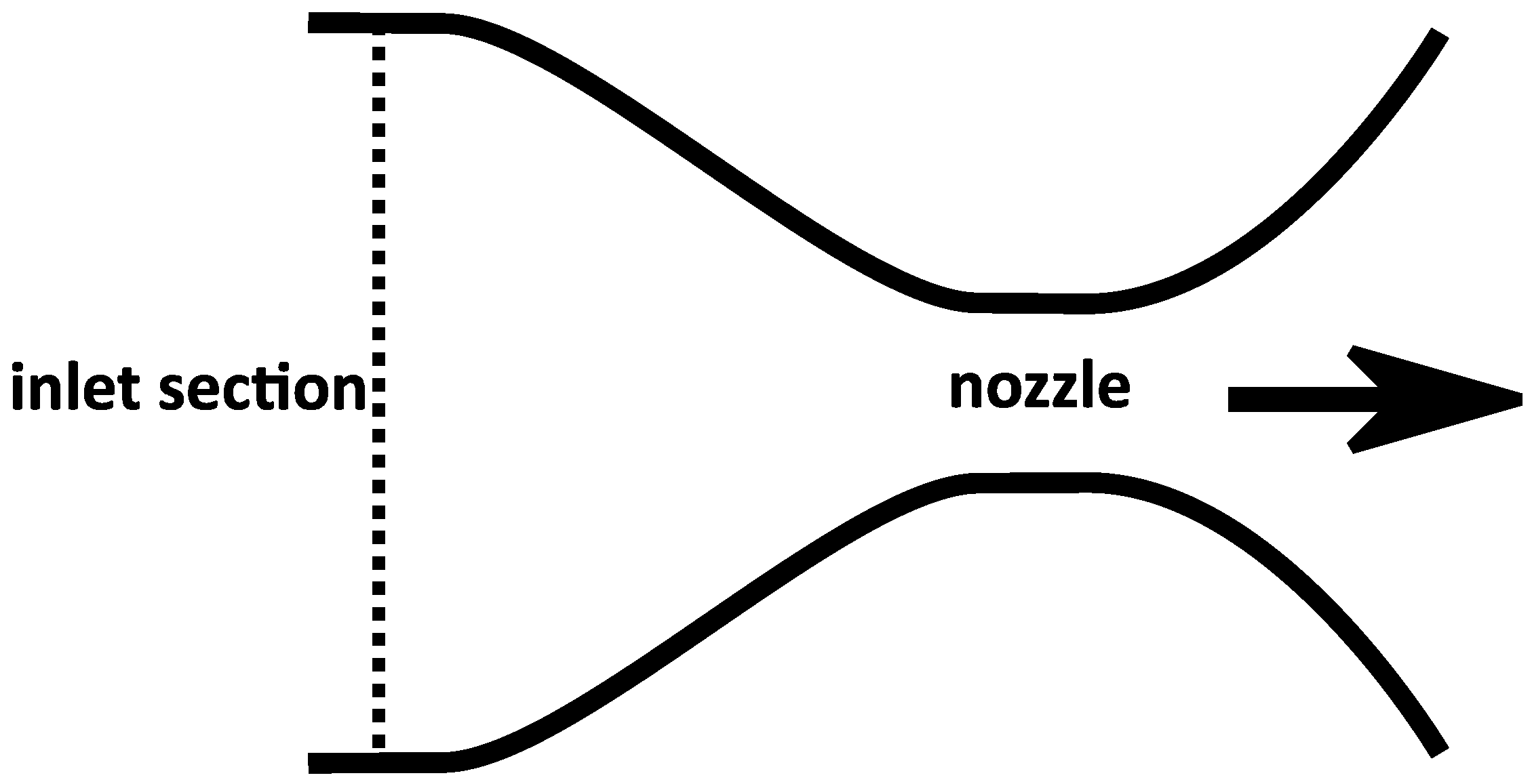
Traditionally, one of the most commonly used models resembles the behaviour of the fluid inside the air valve to the isentropic flow that occurs in a convergent nozzle (Figure 1). Wylie and Streeter [17] made the analogy between nozzles and air valves, where the air behaviour into the pipe is considered isothermal, while the airflow throughout the valve (both inlet and outlet flow) is assumed to be adiabatic.
In this model, the air outlet mass flow G of an air valve, when the flow is subsonic is:
In the Equation (1) Aexp is the air valve output cross section; is the absolute pressure in the pipe upstream the air valve, representing the input pressure p0 in Figure 1; R is the air characteristic constant in the classical thermodynamic formulation of an ideal gas; Tt is the air temperature inside the pipe; is the absolute value of the atmospheric pressure; and Cexp is the outlet characteristic coefficient of the air valve. This coefficient takes values less than one, and the lower the value the higher the airflow resistance.
When the air velocity is greater than the speed of sound (Mach number greater than 1), volumetric flow rate is blocked because speed cannot increase more. Thus, the mass flow rate can be higher since an increase in pressure causes an increase in the density of air. In these supersonic conditions, the mass flow G is:
A similar approach can be carried out in the case of air inlet. In this case, there are two differences. On one side, the pressure in the inlet section is constant and equal to the atmospheric pressure. On the other side, the pressure in the output section is variable. This output section corresponds with the point of the pipe connected with the air valve. Therefore, the air inlet mass flow G, when the flow is subsonic is:
In Equation (3), Cadm is the inlet characteristic coefficient of the air valve, having the same considerations as Cexp in the output process; Aadm is air valve input cross section; and ρatm is the air density at atmospheric conditions.
If the flow is supersonic, the volumetric flow is kept constant. In this case, as the inlet pressure is constant (atmospheric pressure) the mass flow rate also remains constant. Thus, the flow is blocked. This means that even if the pressure inside the pipe decreases more, the amount of air admitted will not increase. Thus, in the conditions of supersonic flow G is:
Expressions (1)–(4) are theoretical formulations of the potential behaviour of an air valve. The real behaviour of the air valve must be obtained through tests, and this information should be provided by the manufacturer. As an example, Figure 2 shows a graph built from the technical information provided by a manufacturer.
Often, simplified expressions are used to treat numerically the characteristic curves of an air valve instead of the previous theoretical equations. The need to simplify these equations is related to decreasing the number of parameters on which the behaviour of the device depends. In this regard, Boldy [18] proposes a representation based on the equations of incompressible flow. Later, Fuertes [3] performed a comprehensive review of the different models representing the behaviour of an air valve. All simplified models seek to reduce the number of parameters needed to characterize this, setting a relationship between the mass flow admitted or expelled and the pressure inside the pipe.
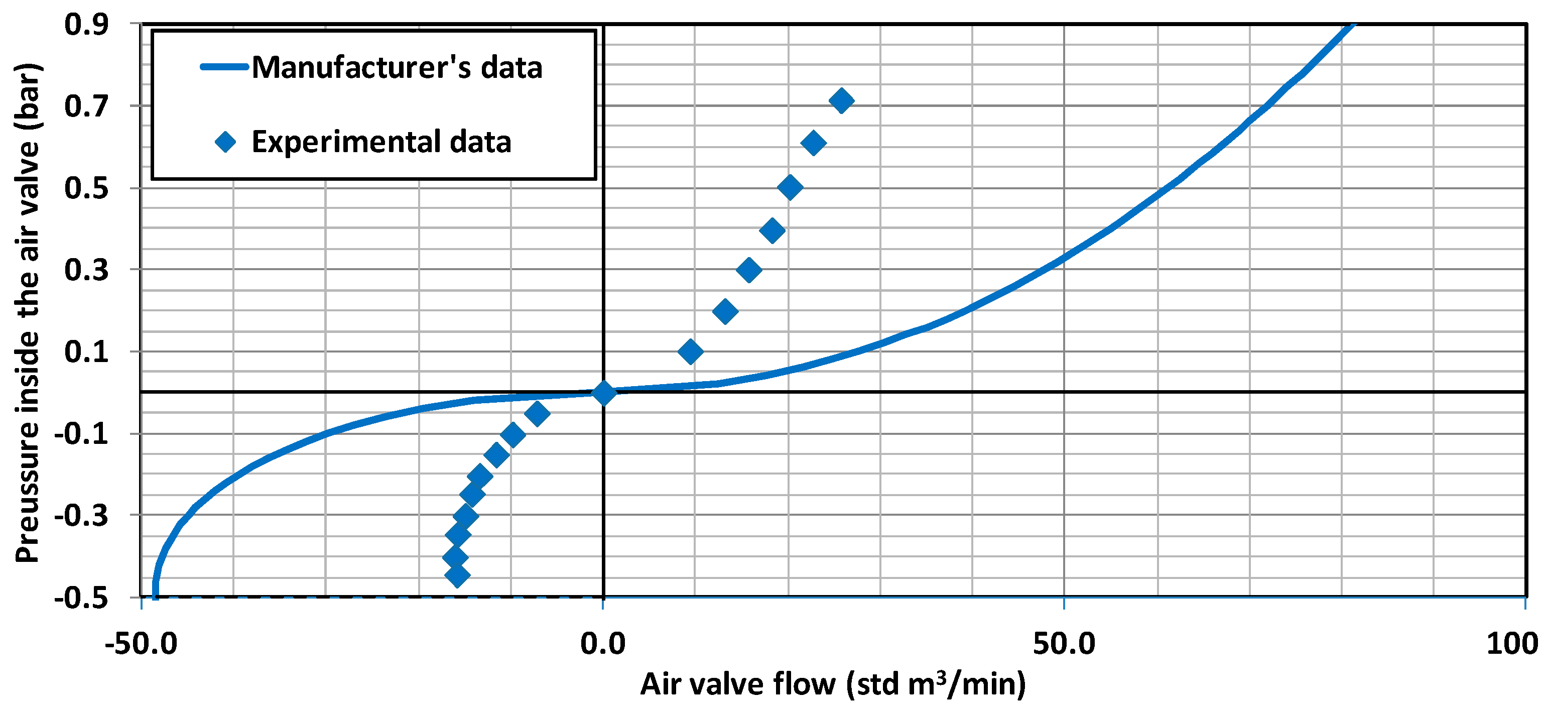
Normally, the manufacturers of air valves present a graph of the characteristic curve. This is the ratio between the admitted/ejected airflow and the difference in pressure between the inside and outside of the air valve. This curve is obtained with experimental tests in all possible operating regions. It is possible to obtain some equations from it, which relate the airflow to the difference in pressures. Unfortunately, the conditions under which these tests are performed are often not referenced in the technical information provided by the manufacturers, so it is nearly impossible to reproduce these tests in a laboratory. In fact, previous studies [3] have already revealed the discrepancies between the commercial data provided by the manufacturer and the actual data obtained by testing. Figure 3 represents the differences between the experimental data obtained in the laboratory and the curve obtained from the technical information provided by the manufacturer.
Results such as those in Figure 3 shows the need to find methodologies that allow characterizing the behaviour of air valves with sufficient reliability. This work proposes the use of CFD programs as an alternative, because these techniques are now considered as standard tools to predict the fluid flow behaviour. Calculations obtained using CFD will be compared with experimental tests performed in the laboratory.
The main problem of testing the characteristics of an air valve is the volume of air required. A 80 mm air valve can require a flow rate of 6200 m3/h measured under standard conditions. If the size is 100 mm the required flow is 9700 m3/h, while for 300 mm it may be necessary up to 87,000 m3/h.
Currently there are two main techniques to test an air valve. The first is based on the storage of large quantities of air in high pressure tanks. During the test the air is released gradually through a system that reduces the pressure to the usual operating pressures of these elements. The difficulty of this system is the tank volumes required are very high (32 m3 for 100 mm and almost 300 m3 for a 300 mm). An alternative option is to use a blower capable of providing the flow and pressure necessary to perform the test. The problem with these installations is the cost associated with the construction of this type of equipment. Simply as a reference data, to test a 300 mm air valve capable of dealing 24 m/s with a pressure of 0.9 bar, requires an approximate power of 1.4 MW. This data is an indicator of the complexity of this type of facility and justifies the fact that there are few places to carry out this type of test.
The experimental study was conducted at the Air Valves Test Bench of Bermad (Israel). This installation has a blower of 315 kW with capacity of 16,000 m3/h of air measured in standard conditions a 0.6 bar of differential pressure. At each test point the flow stability conditions were verified and subsequently the mass flow rate and the pressure at the inlet were recorded. The measuring devices have been previously calibrated guaranteeing errors below 0.5%. The system complies with all European standards and allows the testing of air valves between 2 and 12 inches in a continuous process that allows the measurement of air flow over the entire range of pressures considered. More details about the test bench and the collected data can be found in [16].
In this case, the tests were carried out on more than 20 different models from 13 different manufacturers, with flow ranges between −2500 and 3500 m3/h and pressure ranges between −0.57 and 0.58 bar. All the elements tested were air/vacuum valves 80 mm diameter, capable of exhausting air during pipeline filling and admitting large amounts of air if pressure drops below atmospheric.
3. Computational Fluid Dynamics (CFD) Modelling
CFD means the use of a computer-based tool for simulating the behaviour of systems involving fluid flow, heat transfer, and other related physical processes. CFD works by solving the Navier–Stokes equations over a region of interest, describing how the different properties (velocity, pressure, temperature, density, etc.) of a moving fluid change. CFD is used by engineers and scientists in a wide range of fields, including motor industry (combustion modelling and aerodynamics), buildings (thermal comfort, fire effects, or and ventilation), electronics (heat transfer within and around circuit boards) or medical applications (cardiovascular medicine). In recent years, CFD models have been applied for solving several hydraulic engineering problems. In this way, CFD has been used for a variety of purposes, as simulations of flow transient in pipes [19,20], behaviour of different control valves under different conditions [21,22,23,24], mixing models in water distribution systems [25,26,27,28], or for the characterization of elements in open channels [29,30,31,32,33,34].
CFD allows the analysis of flow patterns that are difficult, expensive or impossible to study using experimental techniques and although they cannot completely replace the measurements, the amount of experimentation and the overall cost can be significantly reduced. In addition, the level of detail that can be achieved with these techniques is very high, generating a lot of additional information without added costs. This allows more complex and complete studies of those that can be performed experimentally.
CFD techniques also have a number of disadvantages. On the one hand, the results of a CFD simulation are not 100% reliable, since it is necessary to simplify real physical systems and properly model complex phenomena such as turbulence. On the other hand, the CFD techniques require computers with great calculation capacity. Since computer capabilities have increased in the last years, CFD techniques provide a tool for determining the pneumatic characteristics of an air valve.
To perform a CFD analysis, there are three main stages: pre-processing, simulation and post- processing. The pre-processing step includes geometry definition, mesh generation and boundary conditions definition. Once the physics problem has been identified, the simulation stage consists in solving the governing equations related to flow physics problems. Finally, the post-processing is the analysis of the results.
The geometry definition consists of specifying the shape of the physical boundaries of the fluid. Among other issues, it is necessary to define whether the computational model will be two-dimensional or three-dimensional. In this work, a standard computer-aided design (CAD) program is used to model a 3D commercial air valve. It should be noted that it is not necessary to include all the details of the air valve. Thus, given that the nominal diameter of the element is 80 mm, details of the geometry of size less than 1 mm have not been considered. Additionally, the geometry of the air valve (Figure 4) has been considered, so only half of it is represented. Likewise, in order to guarantee that the inflow into the air valve has been established, a straight pipe of the length equal to four diameters has been defined at the entrance.
The second step is mesh generation, which consists in dividing the domain of the fluid into a number of smaller cells. The solver used (ANSYS Fluent) is based on the finite volume method, where the domain is divided into a finite set of control volumes. The general conservation equations for mass and momentum are solved on this set of control volumes.
For the representation of the behaviour of the air valves, a structured tetrahedral mesh has been selected, since this type of mesh allows a better adjustment than the hexahedral meshes, especially in the curved areas of the interior of the valve. In order to ensure proper convergence of the model, a preliminary analysis of the minimum mesh size required was performed. This analysis is performed considering the following boundary conditions: the mass flow rate of air is fixed in the inlet while the pressure remains constant in the output. Specifically in this study the required pressure at the inlet of the valve to generate a flow of 2000 m3/h of air under standard conditions, i.e., a mass flow of 0.667 kg/s, has been calculated.
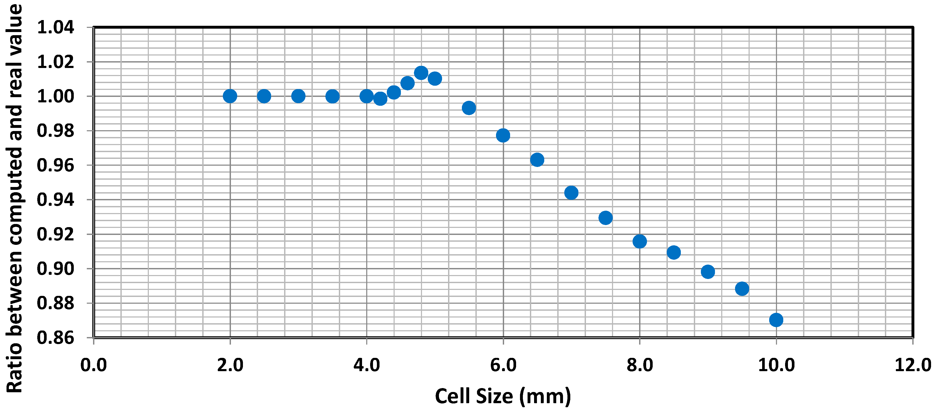
All the simulations have been carried out by means of an implicit formulation in steady state. The resolution algorithm uses a density-based method, which has a coupled formulation of the equations of continuity, momentum and energy. This method of resolution allows better representation of the flow than pressure-based algorithms since the latter erroneously characterize negative pressure gradients. The numerical results of the convergence analysis of the mesh are collected in Table 1, where the value of the pressure P required at the inlet of the suction cup is shown based on the reference size used in the mesh and the number of elements it contains. As can be seen in Figure 5, mesh sizes around 4 mm are enough to analyze this type of problem with an adequate level of accuracy. Consequently, considering at least 300,000 cells guarantees an analysis with sufficient precision, as can be seen in Figure 6.
Since a tetrahedral mesh has been used instead a hexahedral mesh, it has been necessary to review the aspect ratio of the different mesh elements. For the cell reference size finally selected (4 mm), 95% of the elements have a ratio of less than 2.5. Although only 5% of the cells have higher values, considering that less than 0.5% of the elements have an aspect ratio greater than 4.
The equations that describe the properties and motion of the fluid are numerically solved in each of the defined mesh cells. In general, these equations are obtained by applying the equations of continuity and momentum. The application of these laws allows obtaining the Navier–Stokes equations, which for a compressible flow, such as the air inside an air valve, can be expressed in a simplified way such as:
where ρ is the density of the fluid, is the velocity field, p is the pressure field, g are the forces per unit volume to which the fluid is subjected and is the stress tensor.
The Navier–Stokes equations are analytical and in order to solve them with a computer it is necessary to convert them into an algebraic system. This process is known as numerical discretization and there are different methods, being the most used finite difference, finite elements and finite volume.
Another of the basic aspects to consider when performing CFD analysis is the definition of the turbulence model. The objective of the turbulence models for the Reynolds-averaged Navier–Stokes (RANS) equations is to compute the Reynolds stresses and this is one of the basic aspects to consider when analyzing a flow through CFD.
There are several different formulations for solving turbulent flow problems such as Spalart–Allmaras, k-epsilon, k-omega, Menter´s Shear Stress Transport models, etc. All of these models increase the Navier-Stokes equations with an additional viscosity term. The differences between them are the use of wall functions, the number of additional variables solved and what these variables represent.
This work uses a k-ε two-equation turbulence model introduced by Launder and Spalding [35], where k is the turbulent kinetic energy and ε is the rate of dissipation of kinetic energy. The k-ε model has great applicability to turbulent air and water flows and is very popular for practical engineering applications, due to its good convergence and relatively less computational requirements, obtaining results with comparable accuracy to higher order models.
Actually, the k-epsilon model would be more properly called a family of models, because some variants have been developed for so many specific flow configurations. In this work, a feasible k-ε realizable model has been used, where the term realizable means that the model satisfies certain mathematical constraints on the Reynolds stresses, consistent with the physics of turbulent flows. The modelled transport equations to find the terms k and ε are:
In Equations (7) and (8) uj represents velocity component in corresponding direction (xj); μt is the absolute dynamic viscosity of the air; Gk is the turbulent kinetic energy generated by the variations of the mean flow velocity components; Gb represents the kinetic energy generated by the buoyancy effects; YM is the contribution of the pulsatile expansion associated with the compressible turbulence; C1ε, C2 and C3ε are constants; σk and σε are the Prandl numbers for k and ε respectively; and Sk and Sε represent a global variation in time of the parameters k and ε, being defined independently of the rest of variables. Likewise, the constants C1, η and S are defined by:
On the other hand, turbulent viscosity µt is calculated by a combination of k and ε by the equation:
where Cµ is a constant.
In this model, the constants C1ε, C2, C3ε, σk and σε are adopted from the values proposed by Launder and Spalding [35], since this proved that they are very effective for turbulent flows with a wide range of Reynolds number for both water and air. The realizable model has shown some improvements over the standard k-ε model, because it predicts more accurately the spreading rate of both planar and round jets. Likewise, it has also been shown that it performs better in flows involving rotation, boundary layers under strong adverse pressure gradients, separation and recirculation.
For a complete treatment of this problem, properties, initial and boundary conditions of the flow in space and time, would need to be specified. Regarding the properties of the fluid, it is necessary to specify viscosity, density and thermal properties. Regarding the flow inside the air valve, the viscosity of the air is considered constant, while the density varies admitting an air behaviour as if it were a perfect gas.
As initial conditions initial values for the variables are considered, from which the iterative process begins. The closeness of these initial values to the final solution has an influence on the process convergence time. In this work the initial pressure value is equal to the atmospheric pressure, while the initial air velocity is zero at all points.
The boundary conditions control the value of the variables or their relationship in the domain limits analyzed. It is basically about setting fixed values of pressure, velocity and temperature. On the model of an air valve of this work, the pressure is kept constant at the entrance and the exit. To analyze the air expulsion, this fixed inlet pressure will change in the different simulations, while the pressure in the outlet section will be constant and equal to the atmospheric pressure.
Once the model input values are completed, the software can solve the equations for each cell until an acceptable convergence is achieved.
The convergence of the method is based on the analysis of different criteria. Thus, as a general rule, the error is required to be less than 10−3 in the continuity equation, in all the Navier–Stokes momentum equations for each direction (x, y, z), and in the model-specific equations of turbulence (k and ε in this case). Additionally, given the compressible nature of the fluid, the use of the energy equation is required. In this case, the degree of convergence is more demanding (10−6) than in the rest of convergence equations. Likewise, the fulfillment of a certain value of the residuals of the equations is not enough. Therefore, in order to ensure the convergence of the method, stability is required in the values of both the pressure at the inlet of the air valve and the mass flow that circulates inside the valve.
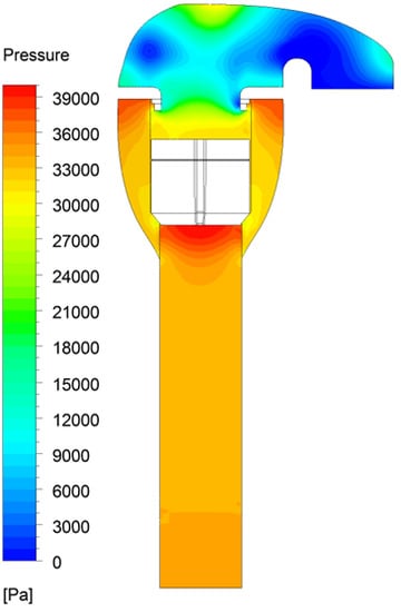
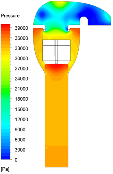
Finally, a post-processing software included in ANSYS is used to analyse the results generated by the CFD analysis. The data obtained can be analysed both numerically and graphically. In general, the most interesting graphic results that can be obtained is the distribution of pressures inside the air valve (Figure 7).
Figure 7 allows analyzing in detail the different parts of the interior of the air valve where greater energy is lost. From the point of view of the design of the device, these zones are enlisted in areas where the pressure gradients are greater. Undoubtedly, improving the capacity of admission or expulsion of an air valve involves improving the design of these points. However, the objective of this work is not the design of this type of device, but to determine the capacity of the CFD techniques to predict their capacity of admission and expulsion.
4. Results
The application of the described analytical methodology allows comparing results obtained computationally with those obtained experimentally. For the particular case of one of the air valves studied, the results considering air as expulsion flow are shown in Figure 8 and Figure 9.
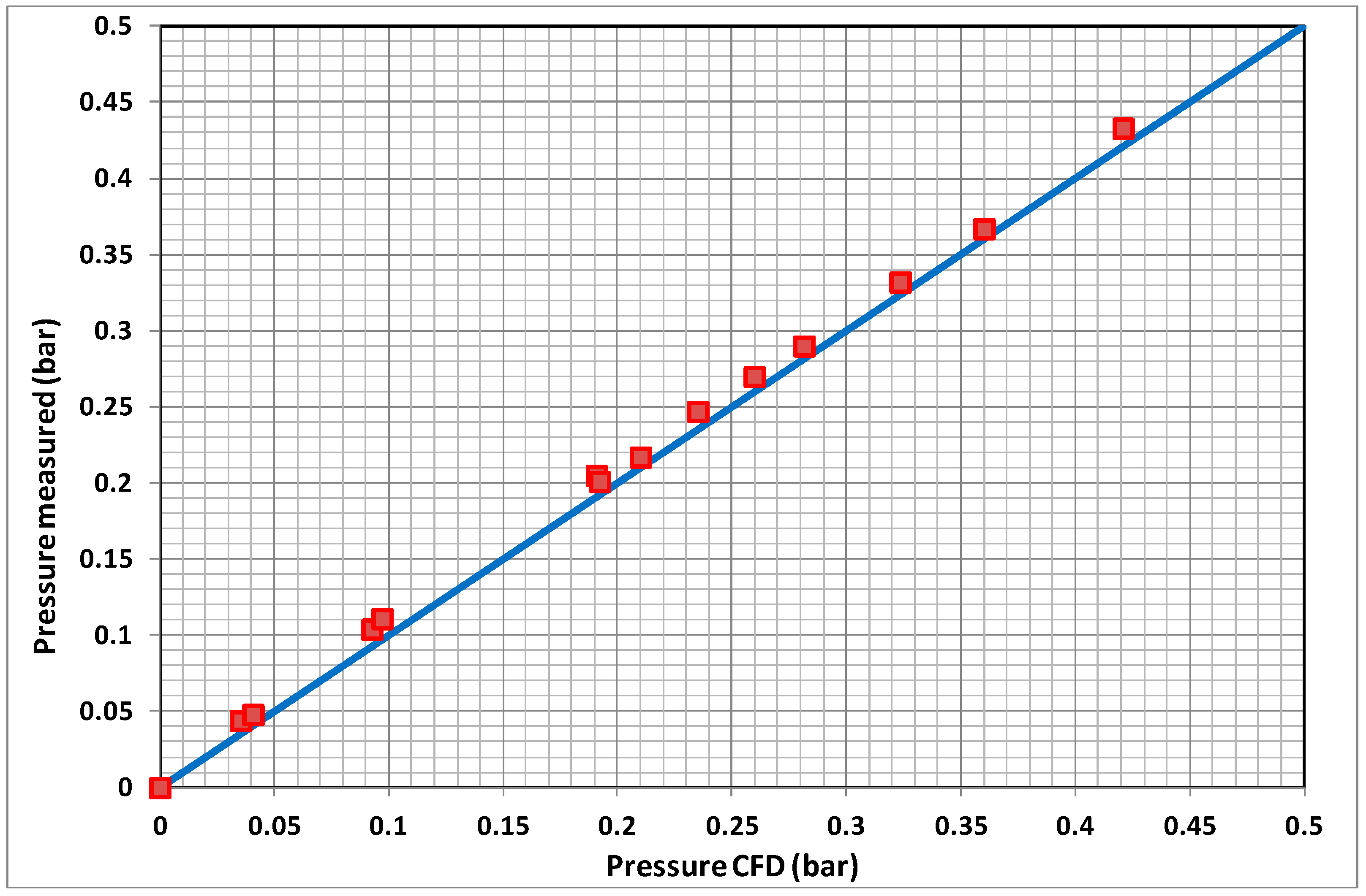
The Figure 8 considers the representation of pressure and flow values. This representation demonstrates the good correspondence between the results obtained through the CFD simulation and the results obtained through laboratory tests. Additionally, Figure 9 represents the pressure values of the CFD results against the laboratory tests. This allows comparing both methodologies in a more detailed way. The results demonstrate the validity of the methodology based on CFD to be able to predict the behavior of an air valve.
Even considering the goodness of the results in Figure 9, to validate the CFD-based methodology of this work as an adequate technique for representing air inlet and outlet characteristics in an air valve, two additional questions need to be answered. On the one hand, it is necessary to validate the methodology for other geometries. On the other hand, it is also required to validate the method when it is applied in the case of air intake from the outside to the inside of the pipeline.
Related to this, the CFD analysis was performed on six different models of air valves of the same nominal diameter (DN 80 mm) but with different internal configurations and different air outlet mechanisms (down, side, mushroom). The results of these analyses are presented in Figure 10.
The results show a good fit between CFD simulations and laboratory tests. However, all tests are performed up to a certain maximum pressure value. This maximum pressure is conditioned in each case for different reasons. In some cases, some of the air valves did not allow further extension of the air expulsion tests, since the flow that causes the dynamic closing of the valve was reached. That is to say, the air valve closes without the presence of water simply by the efforts caused by the air current that overcome the weight of the float. In other cases, the analysis is not extended because the maximum capacity of the test equipment is reached, which is 3000 m3/h of free air or 0.5 bar of differential pressure.
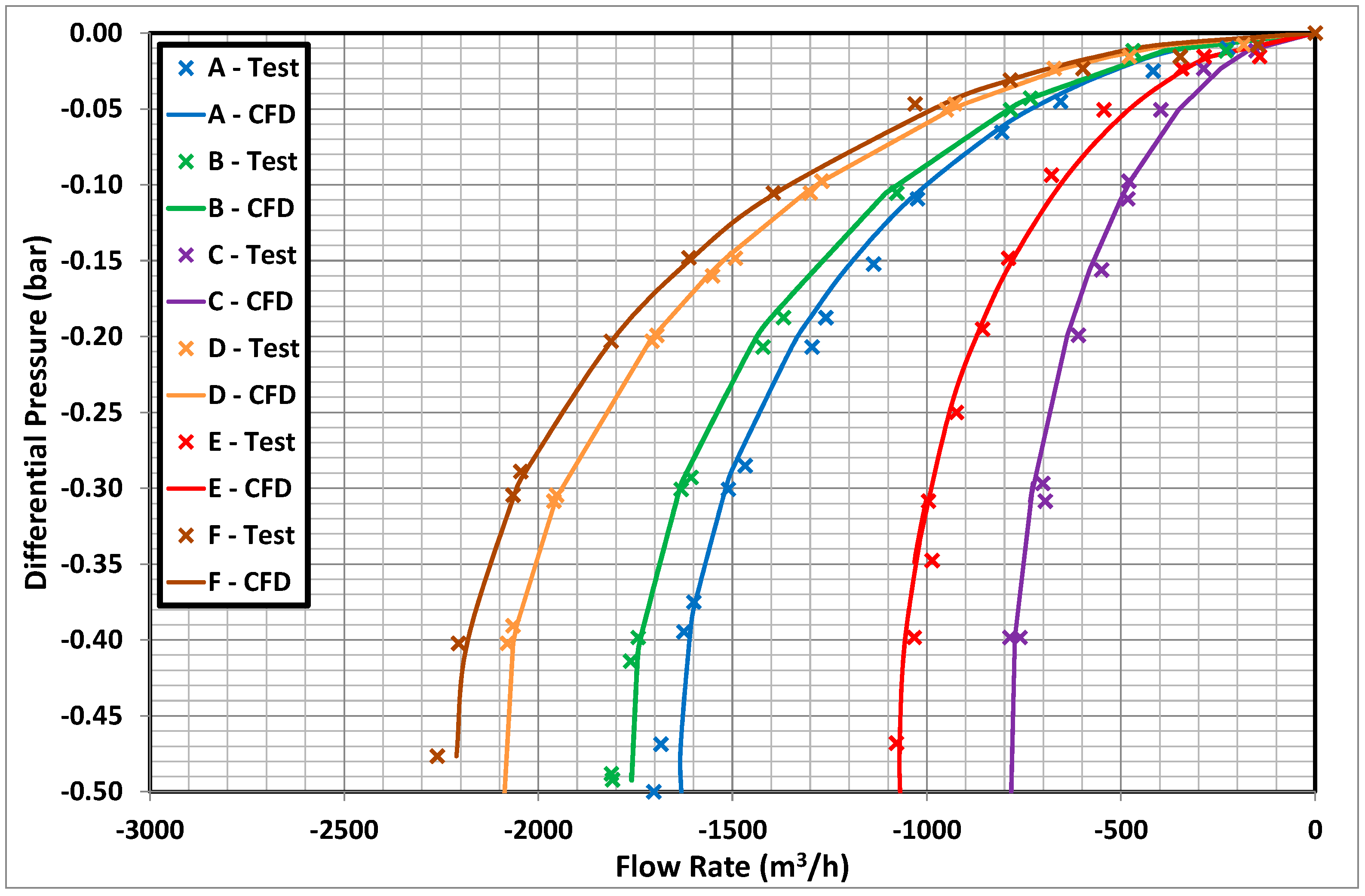
Once the capacity of the CFD model to represent the behavior of the air valve in ejection is verified, the process is repeated in the case of air intake. It should be noted that the compressibility effects of air are more noticeable when the pressures are lower. In this sense, it is important to highlight the capacity of the CFD model to represent the sonic block that is reached in the air valve when the pressures approach values close to −0.5 bar.
Figure 11 shows the results of the comparative study of six models of air valves in the intake phase. As can be observed, there are hardly any differences between the results obtained by laboratory tests and by CFD techniques.
As in the study of the expulsion of air, there is an analysis limit of 0.5 bar differential pressure between the outside of the pipeline and the inside of the pipeline. There are two reasons for this limitation of the study. The first is the maximum test capacity of the test bench used. The second is that for differential pressures greater than 0.5 bar below atmospheric pressure, the so-called sonic block is produced. In other words, the volumetric flow admitted by the suction cup reaches its maximum value. Consequently, as shown in Figure 11, both the results of the CFD model and the laboratory tests tend asymptotically to a value of maximum intake flow and this value will not increase although the depression inside the conduction increases.
5. Conclusions
CFD techniques provide a tool for determining in detail the behavioral characteristics of hydraulic elements. However, CFD requires a proper calibration of the models, so it will be essential to validate the results by tests in the laboratory. Specifically, this work shows the effectiveness of these techniques to represent the behavior of air valves that are installed in water supply networks. According to the results, it is possible to state the following:
- The size and quality of the mesh play a key role in the stability and accuracy of numerical calculations. The computational results of this work in 80 mm air valves reproduce accurately the laboratory tests with meshes from 250,000 elements, which is equivalent to a reference size equal to or less than 4 mm for each cell. The lower quality meshes introduce significant errors in the analysis, even higher than 10%.
- The CFD model has successfully represented the processes of air expulsion in an air valve, obtaining practically the same results in computer simulations as in laboratory tests. However, the CFD analysis does not allow prediction of the dynamic closure of the air valve. This dynamic closure has only been validated through laboratory tests. This is the reason why in some cases the curves of the air valves obtained through CFD cover a range of flow greater than those obtained experimentally.
- CFD models have been very effective representing the behavior of air valves during intake processes, where compressibility phenomena are more important. The CFD techniques can predict the behavior of the air valves in admission and specifically represent the sonic block when depressions close to 0.5 bar are reached. Under these circumstances, both the tests and the CFD simulations indicate the presence of a maximum flow rate that the air valve can accept.
- The discrepancies between the CFD model and the laboratory tests are lower than the error levels of the measuring devices used, in practically all the cases analyzed. Therefore, the correlation between the two techniques can be considered good. This undoubtedly highlights the adequacy of the type and size of mesh selected and the selected turbulence model.
To summarize, it can be concluded that the CFD models are an efficient alternative to represent the air valves during the entry and exit of air to the system. Given the difficulty and the costs of testing this type of element, the application of these techniques is an adequate alternative for the characterization of these elements. In the same way, the methodology could be very useful to verify the technical information provided by the manufacturers.
Author Contributions
All authors contributed extensively to the work presented in this paper. S.G.-T., P.L.I.-R. and D.M.-M., contributed to the subject of research, the modelling, the data analysis, and the writing of the paper. F.J.M.-S. and V.S.F.-M. contributed to the experimental measures and the manuscript review.
Funding
This research was funded by the Program Fondecyt Regular, grant number 1180660.
Acknowledgments
This work was supported by the Program Fondecyt Regular (Project 1180660) of the Comision Nacional de Investigación Científica y Tecnológica (Conicyt), Chile.
Conflicts of Interest
The authors declare no conflict of interest.
Abbreviations
The following abbreviations are used in this manuscript:
| CFD | Computational Fluid Dynamics |
| RANS | Reynolds-averaged Navier–Stokes |
References
- Martin, C.S. Entrapped air in pipelines. In Proceedings of the 2nd International Conference on Pressure Surges; BHRA Fluid Engineering: London, UK, 1976; Volume 2, pp. 15–27. [Google Scholar]
- Liou, C.P.; Hunt, W.A. Filling of Pipelines with Undulating Elevation Profiles. J. Hydraul. Eng. 1996, 122, 534–539. [Google Scholar] [CrossRef]
- Fuertes, V.S. Hydraulic Transients with Entrapped Air Pockets. Ph.D. Thesis, Department of Hydraulic Engineering, Polytechnic University of Valencia, Valencia, Spain, 2001. [Google Scholar]
- Zhou, F.; Hicks, F.E.; Steffler, P.M. Transient Flow in a Rapidly Filling Horizontal Pipe Containing Trapped Air. J. Hydraul. Eng. 2002, 128, 625–634. [Google Scholar] [CrossRef]
- Laanearu, J.; Annus, I.; Koppel, T.; Bergant, A.; Vučković, S.; Hou, Q.; Tijsseling, A.S.; Anderson, A.; van’t Westende, J.M.C. Emptying of Large-Scale Pipeline by Pressurized Air. J. Hydraul. Eng. 2012, 138, 1090–1100. [Google Scholar] [CrossRef]
- Apollonio, C.; Balacco, G.; Fontana, N.; Giugni, M.; Marini, G.; Piccinni, A. Hydraulic Transients Caused by Air Expulsion During Rapid Filling of Undulating Pipelines. Water 2016, 8, 25. [Google Scholar] [CrossRef]
- Zhou, F.; Hicks, F.E.; Steffler, P.M. Observations of Air–Water Interaction in a Rapidly Filling Horizontal Pipe. J. Hydraul. Eng. 2002, 128, 635–639. [Google Scholar] [CrossRef]
- Vasconcelos, J.G.; Wright, S.J.; Roe, P.L. Improved Simulation of Flow Regime Transition in Sewers: Two-Component Pressure Approach. J. Hydraul. Eng. 2006, 132, 553–562. [Google Scholar] [CrossRef]
- Li, J.; McCorquodale, A. Modeling Mixed Flow in Storm Sewers. J. Hydraul. Eng. 1999, 125, 1170–1180. [Google Scholar] [CrossRef]
- Ramezani, L.; Karney, B.; Malekpour, A. The Challenge of Air Valves: A Selective Critical Literature Review. J. Water Resour. Plan. Manag. 2015, 141, 04015017. [Google Scholar] [CrossRef]
- Stephenson, D. Effects of Air Valves and Pipework on Water Hammer Pressures. J. Transp. Eng. 1997, 123, 101–106. [Google Scholar] [CrossRef]
- Bianchi, A.; Mambretti, S.; Pianta, P. Practical Formulas for the Dimensioning of Air Valves. J. Hydraul. Eng. 2007, 133, 1177–1180. [Google Scholar] [CrossRef]
- De Martino, G.; Fontana, N.; Giugni, M. Transient Flow Caused by Air Expulsion through an Orifice. J. Hydraul. Eng. 2008, 134, 1395–1399. [Google Scholar] [CrossRef]
- Fuertes-Miquel, V.S.; Iglesias-Rey, P.L.; Lopez-Jimenez, P.A.; Mora-Melia, D. Air valves sizing and hydraulic transients in pipes due to air release flow. In Proceedings of the 33rd IAHR Congress: Water Engineering for a Sustainable Environment, Vancouver, BC, Canada, 9–14 August 2009; IAHR: Vancouver, BC, Canada, 2009. [Google Scholar]
- Bhosekar, V.V.; Jothiprakash, V.; Deolalikar, P.B. Orifice Spillway Aerator: Hydraulic Design. J. Hydraul. Eng. 2012, 138, 563–572. [Google Scholar] [CrossRef]
- Iglesias-Rey, P.L.; Fuertes-Miquel, V.S.; García-Mares, F.J.; Martínez-Solano, J.J. Comparative Study of Intake and Exhaust Air Flows of Different Commercial Air Valves. Procedia Eng. 2014, 89, 1412–1419. [Google Scholar] [CrossRef]
- Wylie, E.B.; Streeter, V.L. Fluid Transients in Systems; Prentice Hall: Englewood Cliffs, NJ, USA, 1993. [Google Scholar]
- Boldy, A.P. The representation and use of air inlet/outlet valves for pressure surge control. In Unsteady Flow Fluid Transients; Watts, J., Bettess, R., Eds.; Balkema: Rotterdam, The Netherland, 1992. [Google Scholar]
- Martins, N.M.C.; Soares, A.K.; Ramos, H.M.; Covas, D.I.C. CFD modeling of transient flow in pressurized pipes. Comput. Fluids 2016, 126, 129–140. [Google Scholar] [CrossRef]
- Zhou, L.; Liu, D.; Ou, C. Simulation of Flow Transients in a Water Filling Pipe Containing Entrapped Air Pocket with VOF Model. Eng. Appl. Comput. Fluid Mech. 2011, 5, 127–140. [Google Scholar] [CrossRef] [Green Version]
- Davis, J.A.; Stewart, M. Predicting Globe Control Valve Performance—Part I: CFD Modeling. J. Fluids Eng. 2002, 124, 772. [Google Scholar] [CrossRef]
- Stephens, D.; Johnson, M.C.; Sharp, Z.B. Design Considerations for Fixed-Cone Valve with Baffled Hood. J. Hydraul. Eng. 2012, 138, 204–209. [Google Scholar] [CrossRef]
- Palau-Salvador, G.; González-Altozano, P.; Balbastre-Peralta, I.; Arviza-Valverde, J. Improvement in a Control Valve Geometry by CFD Techniques. In Proceedings of the ASCE Pipeline Division Specialty Conference, Houston, TX, USA, 21–24 August 2005; American Society of Civil Engineers: Reston, VA, USA, 2005; pp. 202–215. [Google Scholar]
- Lin, F.; Schohl, G.A. CFD Prediction and Validation of Butterfly Valve Hydrodynamic Forces. In Critical Transitions in Water and Environmental Resources Management; American Society of Civil Engineers: Reston, VA, USA, 2004; pp. 1–8. [Google Scholar]
- Romero-Gomez, P.; Ho, C.K.; Choi, C.Y. Mixing at Cross Junctions in Water Distribution Systems. I: Numerical Study. J. Water Resour. Plan. Manag. 2008, 134, 285–294. [Google Scholar] [CrossRef]
- Austin, R.G.; van Bloemen Waanders, B.; McKenna, S.; Choi, C.Y. Mixing at Cross Junctions in Water Distribution Systems. II: Experimental Study. J. Water Resour. Plan. Manag. 2008, 134, 295–302. [Google Scholar] [CrossRef]
- Liu, H.; Yuan, Y.; Zhao, M.; Zheng, X.; Lu, J.; Zhao, H. Study of Mixing at Cross Junction in Water Distribution Systems Based on Computational Fluid Dynamics. In Proceedings of the International Conference on Pipelines and Trenchless Technology (ICPTT), Beijing, China, 26–29 October 2011; American Society of Civil Engineers: Reston, VA, USA, 2011; pp. 552–561. [Google Scholar]
- Ho, C.K. Solute Mixing Models for Water-Distribution Pipe Networks. J. Hydraul. Eng. 2008, 134, 1236–1244. [Google Scholar] [CrossRef]
- Huang, J.; Weber, L.J.; Lai, Y.G. Three-Dimensional Numerical Study of Flows in Open-Channel Junctions. J. Hydraul. Eng. 2002, 128, 268–280. [Google Scholar] [CrossRef]
- Weber, L.J.; Schumate, E.D.; Mawer, N. Experiments on Flow at a 90° Open-Channel Junction. J. Hydraul. Eng. 2001, 127, 340–350. [Google Scholar] [CrossRef]
- Chanel, P.G.; Doering, J.C. Assessment of spillway modeling using computational fluid dynamics. Can. J. Civ. Eng. 2008, 35, 1481–1485. [Google Scholar] [CrossRef]
- Li, S.; Cain, S.; Wosnik, M.; Miller, C.; Kocahan, H.; Wyckoff, R. Numerical Modeling of Probable Maximum Flood Flowing through a System of Spillways. J. Hydraul. Eng. 2011, 137, 66–74. [Google Scholar] [CrossRef]
- Castillo, L.; García, J.; Carrillo, J. Influence of Rack Slope and Approaching Conditions in Bottom Intake Systems. Water 2017, 9, 65. [Google Scholar] [CrossRef]
- Regueiro-Picallo, M.; Naves, J.; Anta, J.; Puertas, J.; Suárez, J. Experimental and Numerical Analysis of Egg-Shaped Sewer Pipes Flow Performance. Water 2016, 8, 587. [Google Scholar] [CrossRef]
- Launder, B.E.; Spalding, D.B. Mathematical Models of Turbulence; Academic Press: New York, NY, USA, 1972. [Google Scholar]
Figure 1.
Isentropic flow in a convergent–divergent nozzle.

Figure 2.
Air valves technical information provided a manufacturer.
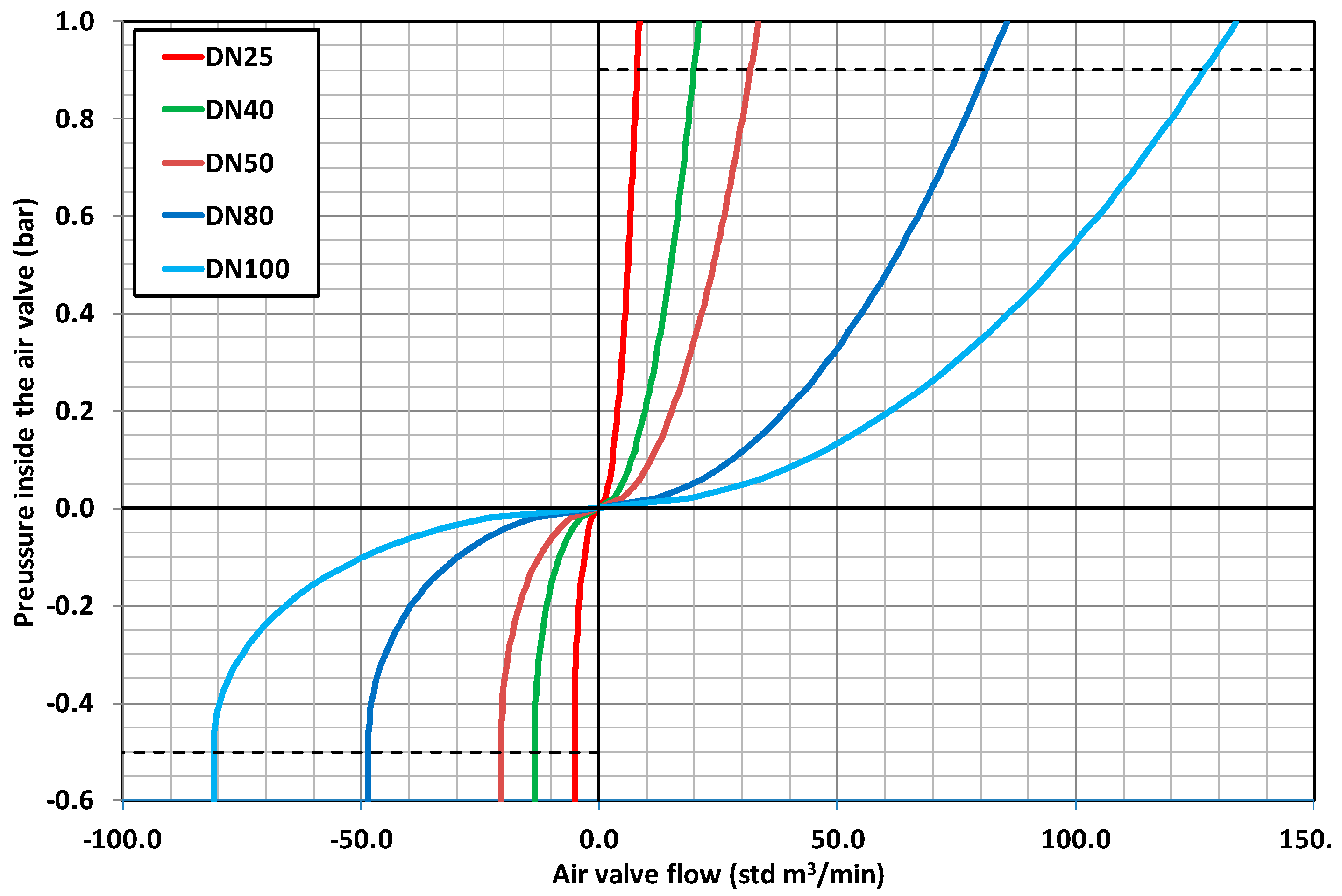
Figure 3.
Comparison between laboratory tests and information provided by a manufacturer.

Figure 4.
Geometry and meshing structure of a commercial air valve for ANSYS Fluent analysis.
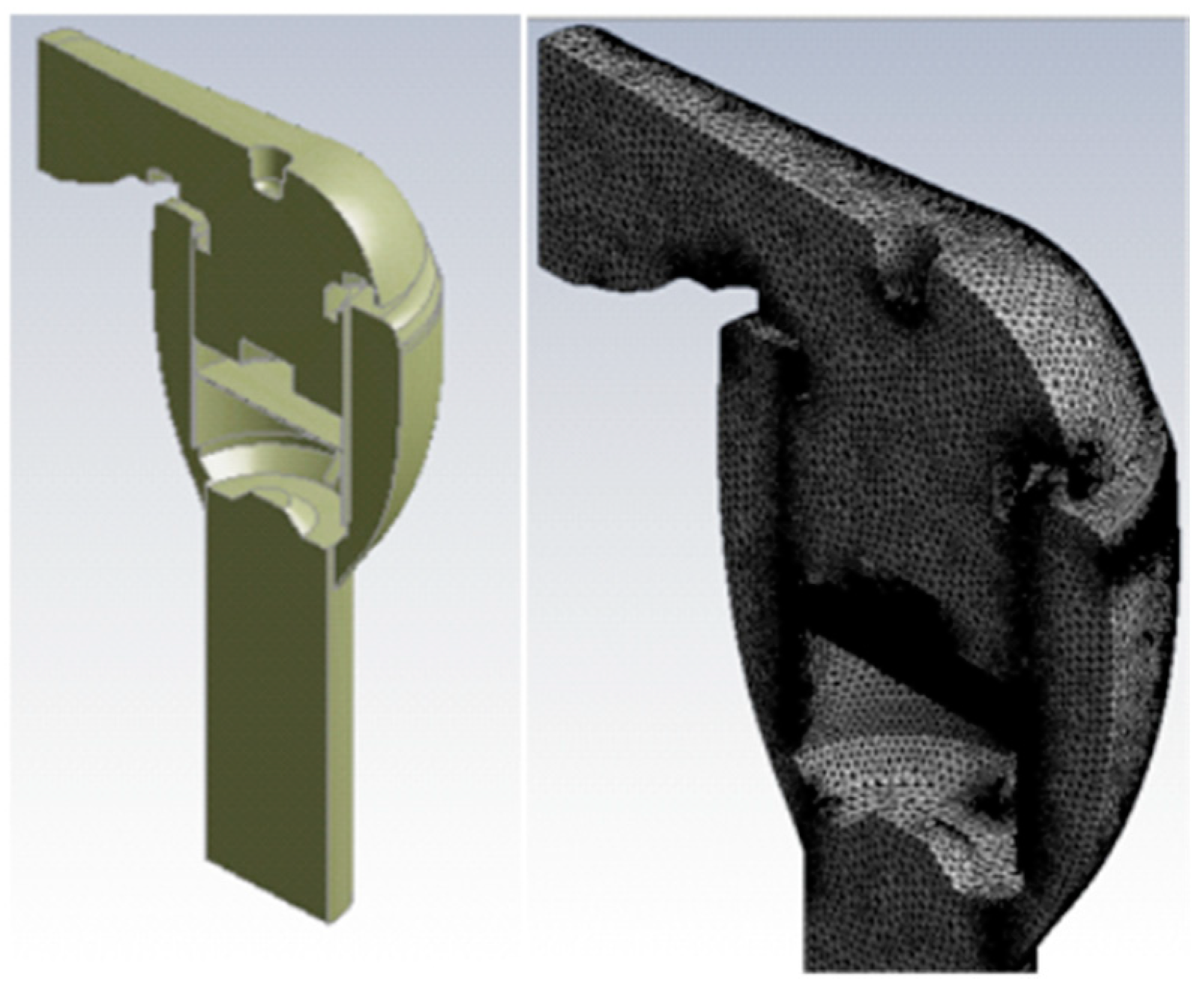
Figure 5.
Analysis of the influence of the size of the mesh (size of the cells).

Figure 6.
Analysis of the influence of the size of the mesh (number of cells).
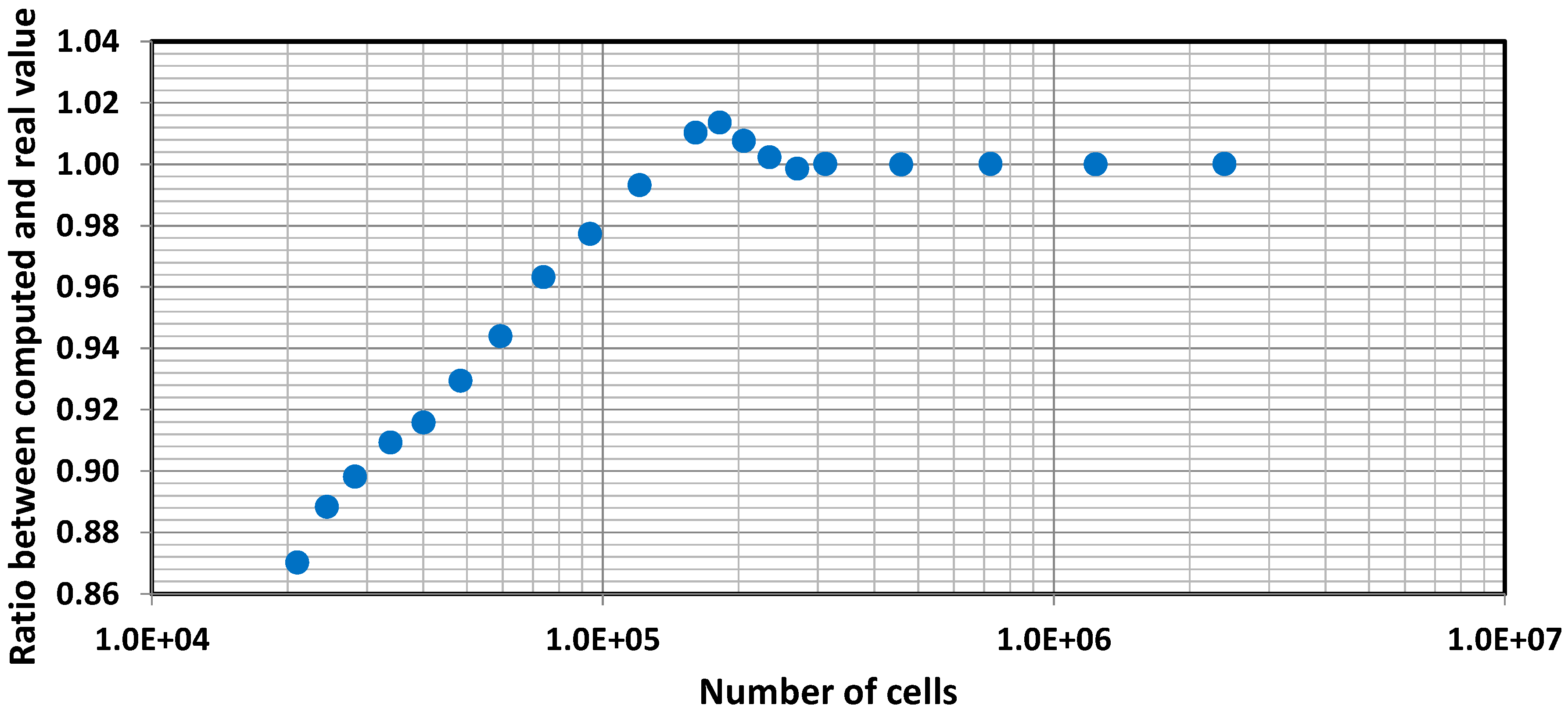
Figure 7.
Pressure distribution in the midplane of the air valve.
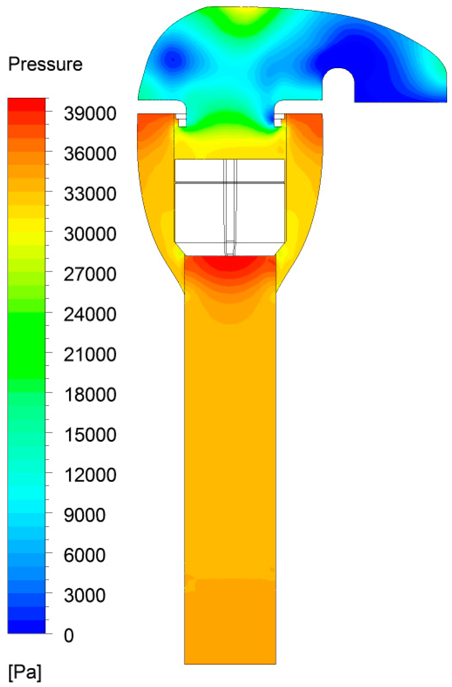
Figure 8.
Comparison of the curve of an air valve: experimental data vs. computational fluid dynamics (CFD) analysis.
Figure 8.
Comparison of the curve of an air valve: experimental data vs. computational fluid dynamics (CFD) analysis.
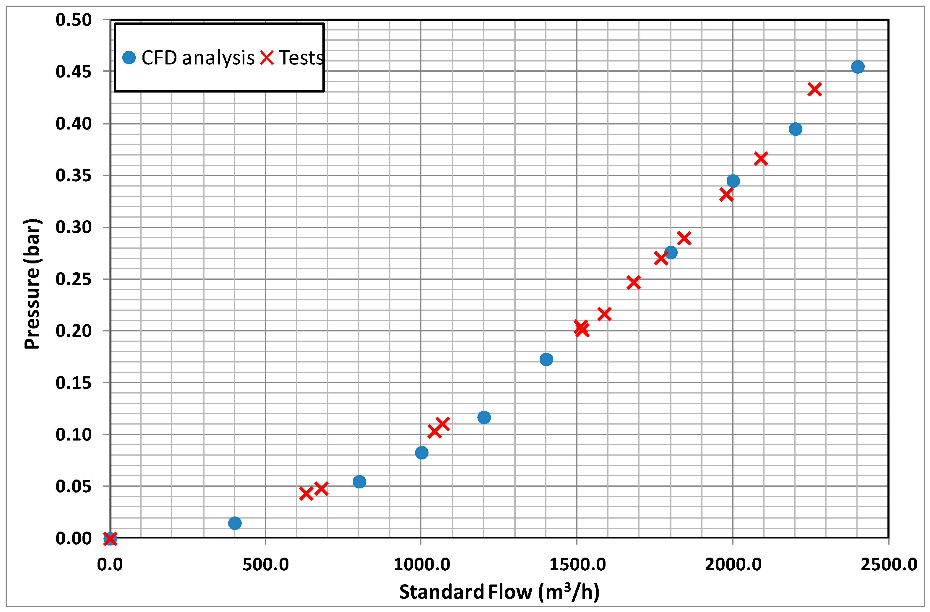
Figure 9.
Comparison of the curve of an air valve: experimental data vs. CFD analysis.

Figure 10.
Comparison between laboratory tests and CFD simulations of six different models of air valve. Air expulsion flow.
Figure 10.
Comparison between laboratory tests and CFD simulations of six different models of air valve. Air expulsion flow.
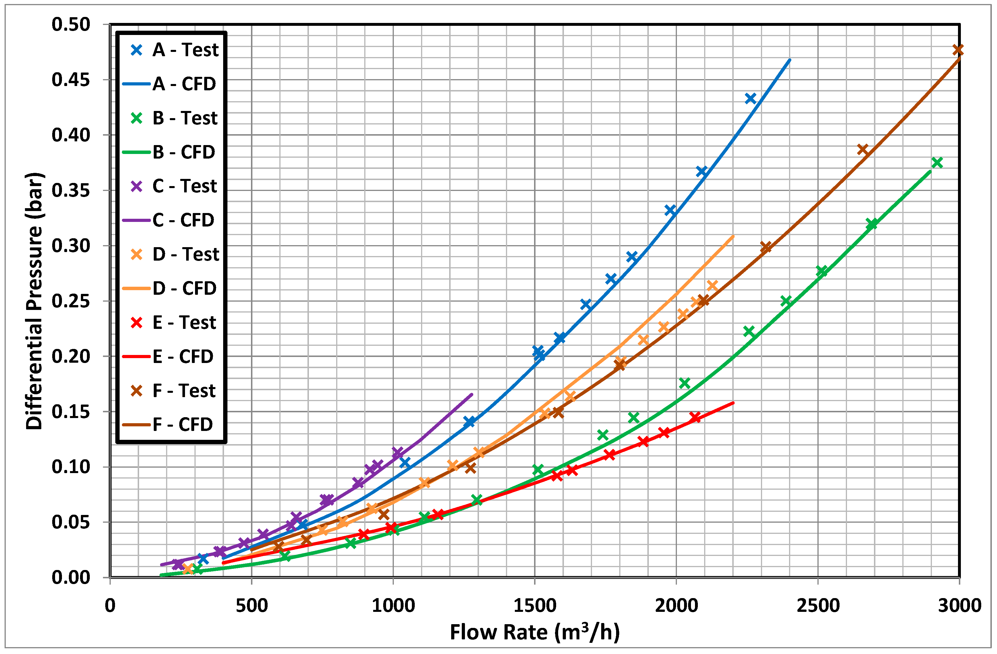
Figure 11.
Comparison between laboratory tests and CFD simulations of six different models of air valve. Air intake flow.
Figure 11.
Comparison between laboratory tests and CFD simulations of six different models of air valve. Air intake flow.

Table 1.
Results of the mesh convergence analysis.
| Size (mm) | No. Elements | P (bar) | Size (mm) | No. Elements | P (bar) | Size (mm) | No. Elements | P (bar) |
|---|---|---|---|---|---|---|---|---|
| 10 | 21,026 | 0.295 | 6 | 93,806 | 0.341 | 3.8 | 363,719 | 0.34 |
| 9.5 | 24,462 | 0.308 | 5.5 | 120,654 | 0.334 | 3.6 | 428,428 | 0.339 |
| 9 | 28,227 | 0.303 | 5 | 160,731 | 0.343 | 3.4 | 507,391 | 0.34 |
| 8.5 | 33,851 | 0.311 | 4.8 | 181,723 | 0.344 | 3.2 | 608,079 | 0.34 |
| 8 | 40,060 | 0.309 | 4.6 | 205,557 | 0.342 | 3 | 738,175 | 0.34 |
| 7.5 | 48,426 | 0.315 | 4.4 | 234,307 | 0.339 | 2.8 | 907,558 | 0.34 |
| 7 | 59,363 | 0.32 | 4.2 | 270,010 | 0.339 | 2.5 | 1,272,477 | 0.34 |
| 6.5 | 73,917 | 0.332 | 4 | 311,827 | 0.339 | 2 | 2,481,359 | 0.34 |
© 2018 by the authors. Licensee MDPI, Basel, Switzerland. This article is an open access article distributed under the terms and conditions of the Creative Commons Attribution (CC BY) license (http://creativecommons.org/licenses/by/4.0/).
Share and Cite
MDPI and ACS Style
García-Todolí, S.; Iglesias-Rey, P.L.; Mora-Meliá, D.; Martínez-Solano, F.J.; Fuertes-Miquel, V.S. Computational Determination of Air Valves Capacity Using CFD Techniques. Water 2018, 10, 1433. https://doi.org/10.3390/w10101433
AMA Style
García-Todolí S, Iglesias-Rey PL, Mora-Meliá D, Martínez-Solano FJ, Fuertes-Miquel VS. Computational Determination of Air Valves Capacity Using CFD Techniques. Water. 2018; 10(10):1433. https://doi.org/10.3390/w10101433
Chicago/Turabian StyleGarcía-Todolí, Salvador, Pedro L. Iglesias-Rey, Daniel Mora-Meliá, F. Javier Martínez-Solano, and Vicente S. Fuertes-Miquel. 2018. "Computational Determination of Air Valves Capacity Using CFD Techniques" Water 10, no. 10: 1433. https://doi.org/10.3390/w10101433
Note that from the first issue of 2016, this journal uses article numbers instead of page numbers. See further details here.