Article

The Performance of Multiple Model-Simulated Soil Moisture Datasets Relative to ECV Satellite Data in China

1
Center for Water Resources and Environment, Sun Yat-sen University, Guangzhou 510275, China
2
Department of Water Resources and Environment, Sun Yat-sen University, Guangzhou 510275, China;
3
School of Information Technology, Shangqiu Normal University, Shangqiu 476000, China
4
Department of Atmospheric Science, School of Environmental Studies, China University of Geosciences, Wuhan 430074, China
5
School of Environmental Science and Engineering, Guangdong University of Technology, Guangzhou 510006, China
*
Author to whom correspondence should be addressed.
Water 2018, 10(10), 1384; https://doi.org/10.3390/w10101384
Submission received: 27 August 2018 / Revised: 28 September 2018 / Accepted: 1 October 2018 / Published: 3 October 2018
(This article belongs to the Section Hydrology)

Abstract

:
Reliability and accuracy of soil moisture datasets are essential for understanding changes in regional climate such as precipitation and temperature. Soil moisture datasets from the Essential Climate Variable (ECV), the Coupled Model Intercomparison Project Phase 5 (CMIP5), the Inter-Sectoral Impact Model Intercomparison Project (ISIMIP), the Global Land Data Assimilation System (GLDAS), and reanalysis products are widely used. These datasets generated by different techniques are compared in a common framework over China in this study. The comparison focuses on four aspects: spatial pattern, temporal correlation, long-term trend, and the relationships with precipitation and the Normalized Difference Vegetation Index (NDVI). The results indicate that all soil moisture datasets reach a good agreement on the spatial patterns of wet and dry soil. These patterns are also consistent with that of precipitation. However, there are considerable discrepancies in the absolute values of soil moisture among these datasets. In terms of unbiased Root-Mean-Square Difference (unRMSE, i.e., removing the differences in absolute values), all modeled datasets obtain performances comparable with ECV observations. Our results also suggest that a multi-model ensemble of soil moisture datasets can improve the representation of soil moisture conditions. The optimal dataset from which the wetting/drying trends in soil moisture have the highest consistency in terms of changes in precipitation and NDVI varies by season. Specifically, in spring, CMIP5 in northwest China shows that the trends in soil moisture are consistent with the changes in precipitation and NDVI. In summer, ECV presents the most identical performance compared to the changes in precipitation and NDVI. In autumn, GLDAS and Reanalysis have better performance in south China and parts of north China. In winter, GLDAS performs the best in the east of south China, followed by the Reanalysis dataset. These discrepancies among the datasets present various changes in different regions, which should be well noted and discussed before use.

1. Introduction

Soil moisture plays a vital role in the land–atmosphere exchange process [1,2,3,4,5]. It governs surface–atmosphere circulation by influencing the material and energy exchanges in the lithosphere, atmosphere, hydrosphere, and biosphere [6,7,8]. It is a fundamental impact factor in modulating soil status, controlling land surface energy partition, adjusting soil drainage and surface runoff, and regulating canopy transpiration and carbon assimilation [9,10]. As an indispensable parameter in all land process models, the estimation of soil moisture can greatly affect the performance of simulation and prediction in hydrology, meteorology, environment, ecology, and agriculture [11,12,13,14,15,16]. Therefore, it is crucial to understand the conditions and changes of soil moisture to elevate scientific knowledge of the changing climate and the accelerated hydrologic circulation.
Reliability and accuracy of soil moisture datasets are essential for investigating different hydrological issues (such as historical and future changes in soil moisture and dynamics of land–atmosphere interactions) and acquiring convincing results. Various techniques have been developed to achieve qualified soil moisture datasets, such as ground-based measurements, remote sensing observations, and model simulations [8,9,17,18]. Although sparse ground-based measurements have been widely used [19], the application of ground-based measurements is commonly limited by the location and number of gauging stations, especially in regions with extensive area and complex geographic features [12,20]. Soil moisture products developed by remote sensing and model simulations in high temporal and spatial resolutions have compensated for the limitations of ground-based measurements effectively. Remote sensing products are various with different active and passive microwave sensors, and include the Advanced Microwave Scanning Radiometer-2 (AMSR2), the Advanced Microwave Scanning Radiometer–Earth Observing System (AMSR-E), the Land Parameter Retrieval Model (LPRM), the Advanced Scatterometer (ASCAT), the Soil Moisture Active Passive (SMAP), and the Soil Moisture and Ocean Salinity (SMOS) soil moisture products [21,22,23,24,25,26,27]. However, individual remote sensing products only cover a short period with several years of records and limited coverage of the globe. The qualities of soil moisture obtained from these products vary among them in terms of temporal changes and spatial coverage [28,29]. Essential Climate Variable (ECV), as a kind of multisatellite merged product, was developed to combine soil moisture datasets with active and passive remote sensing into a normalized scale [30,31,32,33,34,35], which largely breaks through the limitations of individual products.
ECV products provide a more direct estimate of soil moisture increases or decreases based on multiple satellites. Regional studies have proved that ECV products show mode similarity in spatial representativeness with in situ measurements, including validations over American [36], China [37], and southeastern Australia [38]. As for global scale, the accuracy of ECV is acceptable when validated by global ground-based observations with mean correlation coefficient and root-mean-square error (RMSE) of 0.46 and 0.04 cm3/cm3, respectively [31]. On the other hand, more studies have validated the application of ECV products in drought monitoring [39] and soil moisture trend analyses [30,40,41]. Specially, ECV products can reflect the changes in soil moisture caused by irrigated activities in irrigation regions such as north China which are not captured by model simulations [42]. Therefore, some studies point out that ECV has demonstrated potential for evaluating the performances of model simulations [40,43,44]
Due to the limited ability of microwave penetration, the soil moisture in only the top few centimeters can be detected [25,27,45,46,47]. Model-simulated datasets derived by hydrological and land surface models (LSM) have been used to increase the depth for multilayered soil moisture [8,39], including the Global Land Data Assimilation System (GLDAS) [48], the Coupled Model Intercomparison Project Phase 5 (CMIP5) [49], and the Inter-Sectoral Impact Model Intercomparison Project (ISIMIP) [50,51,52,53,54]. Reanalysis datasets produced by data assimilation techniques combine both observations and model simulations [35], such as the European Center for Medium-Range Weather Forecasts Interim Re-Analysis (ERA-Interim) [55], the Modern Era Retrospective analysis for Research and Applications—Land (MERRA) [56], and the Climate Forecast System Reanalysis (CFSR) [57]. However, the high uncertainties and large discrepancies at regional scale among these datasets may largely influence our understanding on the land–atmosphere feedback mechanisms [35,48,58]. Therefore, it is of great importance to analyze the properties of these soil moisture datasets through a comprehensive comparison before using them.
As mentioned for the ECV studies, more works have evaluated the accuracy of these datasets at regional and global scales, such as the evaluation of ASCAT, SMOS, and ECV datasets for the globe [31,59]; the evaluation of ASCAT and AMSR-E datasets in Europe [20]; the comparison of SMOS and CMIP5 datasets in the United States [20,39,60]; and the comparison of GLDAS, SMAP, SMOS, and AMSR2 datasets in the Tibetan Plateau [8,35]. On one hand, these datasets have been demonstrated to have certain abilities to represent the variability and changes in soil moisture. On the other hand, the performances of these datasets vary in different regions with considerable discrepancies. However, a comprehensive comparison of these datasets has not yet been carried out in China.
China, with only 7% of the world’s available arable land, feeds 22% of the world’s population, and the rate of food self-support in China is more than 80%. As crop growth is highly sensitive to the conditions and changes in surface soil moisture, it is crucial to accurately capture the variation of surface soil moisture in China. Therefore, investigating the performances of remote sensing and model datasets for soil moisture across China is important for improving our understanding of agriculture development [28]. In this paper, the objectives of our study are (1) to comprehensively compare a large population of soil moisture datasets generated by different techniques, including ECV, CMIP5, ISIMIP, and GLDAS products, and three Reanalysis datasets (ERA-Interim, MERRA, and CFSR); and (2) to determine which dataset is optimal in specific seasons and regions.

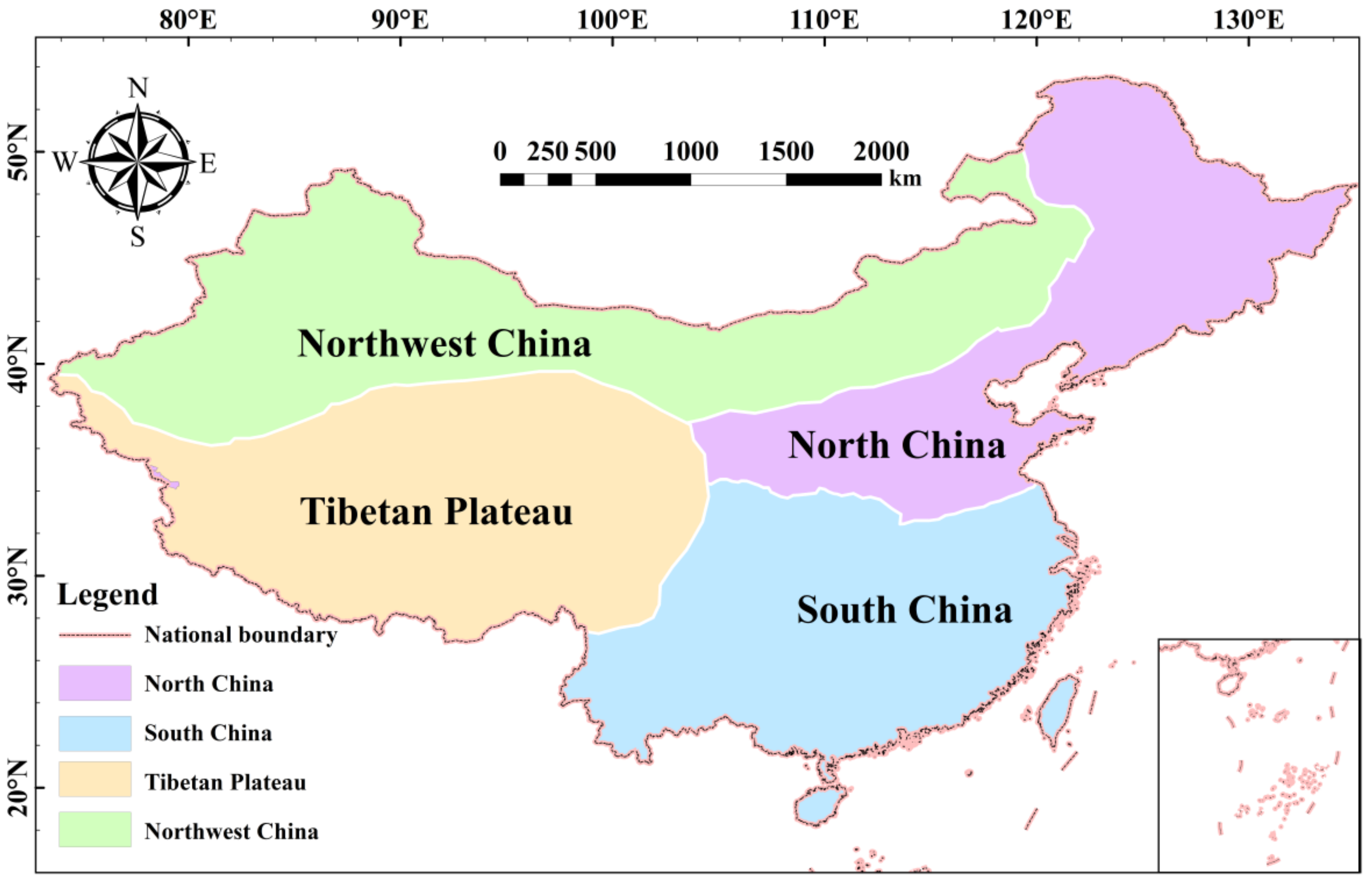
2. Study Area and Data

China has a “terraced” terrain that gradually descends from west to east, and links the mainland and the Pacific Ocean basin through a wide continental shelf. Topography across China varies and is complex, including plains, plateaus, mountains, hills, and basins [37,61]. Considering the complex landforms, diverse climate, and vast latitude and longitude ranges, China can be divided into four types of geographical zones: northwest China, the Tibetan Plateau, south China, and north China (Figure 1) [62]. The performances of soil moisture datasets obtained from ECV, CMIP5, ISIMIP, GLDAS, and Reanalysis are evaluated in the four regions in China.

2.1. ECV Dataset

The ECV datasets provide global surface soil moisture with a spatial resolution of 0.25° and daily temporal resolution spanning over 35 years (from 1978 to 2015). The products are developed as part of the European Space Agency’s (ESA) Water Cycle Multimission Observation Strategy (WACMOS) and Soil Moisture Climate Change Initiative (CCI) projects. The datasets merge the active and passive remote sensing products and scale them into a normalized framework. The active products are two kinds of outputs with coarse-resolution microwave sensors including ERS-AMI and ASCAT (Metop-A and Metop-B). The passive products include the remote sensing outputs from SMMR, SMOS, SSM/I, AMSR-E, TMI, AMSR2, and WindSat. It should be noted that the soil moisture data may fail to be retrieved when the signal (especially the passive signal) is disturbed in regions with dense vegetation (e.g., tropical, boreal forests), complex topography (e.g., mountains), ice cover (e.g., Himalayas), or vast fractional coverage of water [36]. The combination of two active microwave data sources (ERS-AMI and ASCAT) in ECV alleviates significantly the impacts of signal attenuation on soil moisture [31,34]. Compared with earlier versions, the recently released ECV combined soil moisture of version 03.2 extends to 2015. Furthermore, the revisions in ECV 03.2 include improved gap filling, new data attributes, and a revision of processing algorithms [35]. Thus, ECV 03.2 is employed in this paper due to its improved performance. The layer depth of ECV is 0.5–5 cm. The daily ECV under the common period (1980–2005 in Table 1) is averaged into monthly means.

2.2. CMIP5 Soil Moisture

CMIP5 datasets are generated from different general circulation models (GCMs) of CMIP5. All GCMs have different spatial resolutions and temporal lengths. There are two variables for soil moisture: total column soil moisture and soil moisture in the top 10 cm of the soil column [20,49,63]. Most of the GCMs provide the soil moisture information in the top 10 cm, which was used in this study. The GCMs with soil moisture covering the period of 1980–2005 under the historical scenario were selected [16]. Outputs from a total of 37 GCMs are listed in Table 2.

2.3. ISIMIP Soil Moisture

ISIMIP aims to contribute to a quantitative and cross-sectoral synthesis of the differential impacts of climate change. ISIMIP offers a consistent framework for estimating the associated uncertainties in different sectors and at different scales [54]. The ISIMIP soil moisture datasets are outputs of hydrological models in offline mode driven by bias-corrected CMIP5 GCMs. In total numbers from 30 ISIMIP outputs, the soil moisture values from 16 outputs are unrealistically low (i.e., the maximum values are less than 0.05 m3/m3—much smaller than the maximum values of other types of datasets around 0.5 m3/m3). The unrealistic soil moisture outputs are very likely due to systematic errors of the models which are therefore rejected in this study [64,65,66,67,68,69]. The selected ISIMIP outputs are shown in Table 3.

2.4. GLDAS Soil Moisture

The GLDAS is an advanced land surface modeling (LSM) system based on advanced data assimilation techniques [48]. This LSM system incorporates a huge quantity of satellite and ground-based observation data in order to generate optimal simulations of global land surface states and fluxes in near-real time. These LSMs are able to simulate land states and meteorological conditions which include surface air temperature, precipitation, and soil moisture content [18]. Currently, there are two versions of datasets including the GLDAS Version 1 (GLDAS-1) and GLDAS Version 2 (GLDAS-2, not used in this study) [70]. GLDAS-1 drives four offline (uncoupled to the atmosphere) land surface models, i.e., Community Land Model (CLM), Mosaic (MOS), Variable Infiltration Capacity (VIC), and Noah (NOAH), while the GLDAS-2 only involves the NOAH model. More detail can be found in Table 4.

2.5. Reanalysis Soil Moisture

The ERA-Interim, MERRA, and CFSR are three kinds of recently developed global reanalysis datasets. ERA-Interim is a commonly used global atmospheric reanalysis dataset produced by the European Centre for Medium-Range Weather Forecasts (ECMWF). The ERA-Interim assimilates various types of observations including remote sensing and ground-based measurements. This type of dataset considers four layers of soil, including 0–7, 7–28, 28–100, and 100–289 cm [55]). The MERRA assimilates the Goddard Earth Observing System version 5 (GEOS-5, a kind of hydrology LSM) by the NASA (National Aeronautics and Space Application) GMAO (the Global Modeling and Assimilation Office). The MERRA also incorporates information from remote sensing and ground-based measurements to generate datasets with high temporal and spatial resolution. The recent MERRA version 2 includes two layers (0–2 and 0–100 cm) of soil moisture [71]. The CFSR is driven based on the 2009 version of the Noah model in the Global Forecast System (GFS) by the National Centers for Environmental Prediction (NCEP). There are four layers of soil moisture (e.g., 0–0.1 m, 0.1–0.4 m, 0.4–1 m, 1–2 m) obtained from CFSR [72,73]. More information is shown in Table 1 [28,35,71,74,75]. Therefore, monthly soil moistures were extracted from the ERA-Interim with layer depth of 7 cm, MERRA with layer depth of 2 cm, and CSFR with layer depth of 10 cm.

2.6. Precipitation and Vegetation Datasets

Precipitation and vegetation datasets were also used to evaluate the performances of soil moisture datasets in this study. Precipitation is one of the main drivers that largely influences the variations in surface soil moisture [76]. Therefore, the long-term trends in soil moisture were compared with those in precipitation obtained from the Global Precipitation Climatology Centre (GPCC, https://www.dwd.de/EN/ourservices/gpcc/gpcc.html). The GPCC Version 7 merges data from 67,200 stations and various types of satellite observations across the globe. The GPCC precipitation is given in monthly data with a 0.5° × 0.5° spatial resolution from 1901 to present. On the other hand, vegetation evolution is sensitive to root-zone soil moisture. Moreover, the surface soil moisture changes have considerable impacts on the evolution of vegetation. As a proxy for vegetation development, the long-term seasonal NDVI variations have been commonly used to indicate the structural changes in surface soil moisture (the NDVI dataset has higher temporal and spatial resolutions than the vegetation optical depth/VOD) [28,77,78]. The NDVI dataset was obtained from the long-term Global Inventory Monitoring and Modeling Studies (GIMMS) 3 g version (https://ecocast.arc.nasa.gov/data/pub/gimms/). Moreover, the NDVI dataset covers the period of 1981–2016 with a spatial resolution of 1/12° (~8 km at the equator) [79]. Note that soil moisture and precipitation datasets covering the period of 1980–2005 were chosen in this paper.

3. Methods

3.1. Data Inspection

As mentioned in the introduction, ECV agrees well with ground-based observations over different areas. Moreover, the performance of ECV in evaluating model simulations has been validated by previous studies [31,40,43,44]. The performances of modeled soil moisture relative to ECV have been evaluated, and are also in line with previous studies (e.g., Zeng and Chakravorty) [35,75]. Therefore, the ECV was selected as a reference in this comparison. Changing input sensor constellation or natural physical phenomena may lead to data gaps in some periods in ECV [31]. Passive sensors in particular may have difficulty acquiring effective signals in some extremes of weather or terrain [59]. Therefore, it was necessary to inspect data gaps in the ECV data during the period 1980–2005. For regions with pronounced seasonal cycles, such as monsoon regions and continental interiors, the comparison was conducted at annual and seasonal scales (i.e., annual (January–December), MAM (March–May), JJA (June–August), SON (September–November), and DJF (December–February)).
The spatial distribution of record lengths (the years of each grid with available ECV data) of annual and seasonal ECV is shown in Figure 2. The data gaps are mainly located in the Tibetan Plateau and northwest China. The complex terrain in these regions has significant effects on soil moisture retrieval (Figure 2). The data gaps are mainly concentrated in spring (MAM) and winter (DJF), especially winter (DJF, Figure 2). The almost unabridged regions (i.e., the record length > 23 years) are mainly located in the east of southern China, and north and northwest China (Figure 2). To ensure the comparison for a long-term period, the ECV data grids with more than 15 years were considered in this study.

3.2. Data Preprocessing

Soil moisture datasets used in this study have different spatial resolutions, layer depths, lengths, and units, as shown in Table 1, Table 2, Table 3 and Table 4. Hence, preprocessing should be carried out before comparison is conducted among these datasets. Firstly, the layer closest to the surface was selected for comparison in these datasets [8,63]. To guarantee that the datasets were compared in the same period, the surface soil moisture for the period of 1980–2005 was extracted. Secondly, the values of soil moisture were standardized to the volumetric unit (V, m3/m3) by the equation
  V = S h ρ w  
where S is the soil moisture in kg/m2, h is depth of the soil layer in m, and ρw is the density of water in kg/m3. Finally, all datasets were normalized to the spatial resolution of 0.5° × 0.5° using a bilinear interpolation method.

3.3. Statistical Metrics

The mean absolute error (MAE), mean bias error (MBE), root-mean-square error (RMSE), unbiased RMSE (unRMSE), and the Pearson correlation coefficient (r) were used to quantify the agreement between ECV and other datasets. The MAE measures the persistent bias between two datasets. MBE measures the whole averaged bias for different datasets with ECV. RMSE measures the averaged magnitude of the deviation relative to ECV. The unRMSE characterizes the random errors by removing the bias errors [39,75]. The Pearson correlation coefficient between ECV and other datasets provides an indication of the temporal agreement of the datasets [80]. More detailed information about the statistical metrics is shown in Table 5.
Long-term trends in soil moisture are one of the important scientific issues in climate change studies [16,18,30,59]. Therefore, the long-term trends based on different soil moisture datasets are also important metrics for estimating the agreement between different datasets. The trends of precipitation and NDVI are used to evaluate the performances of soil moisture datasets. In this study, the Mann-Kendall test (M-K) was used to examine the trends of soil moisture, precipitation, and NDVI series [81,82]. Significant trends are detected at a significance level of 5%.

4. Results

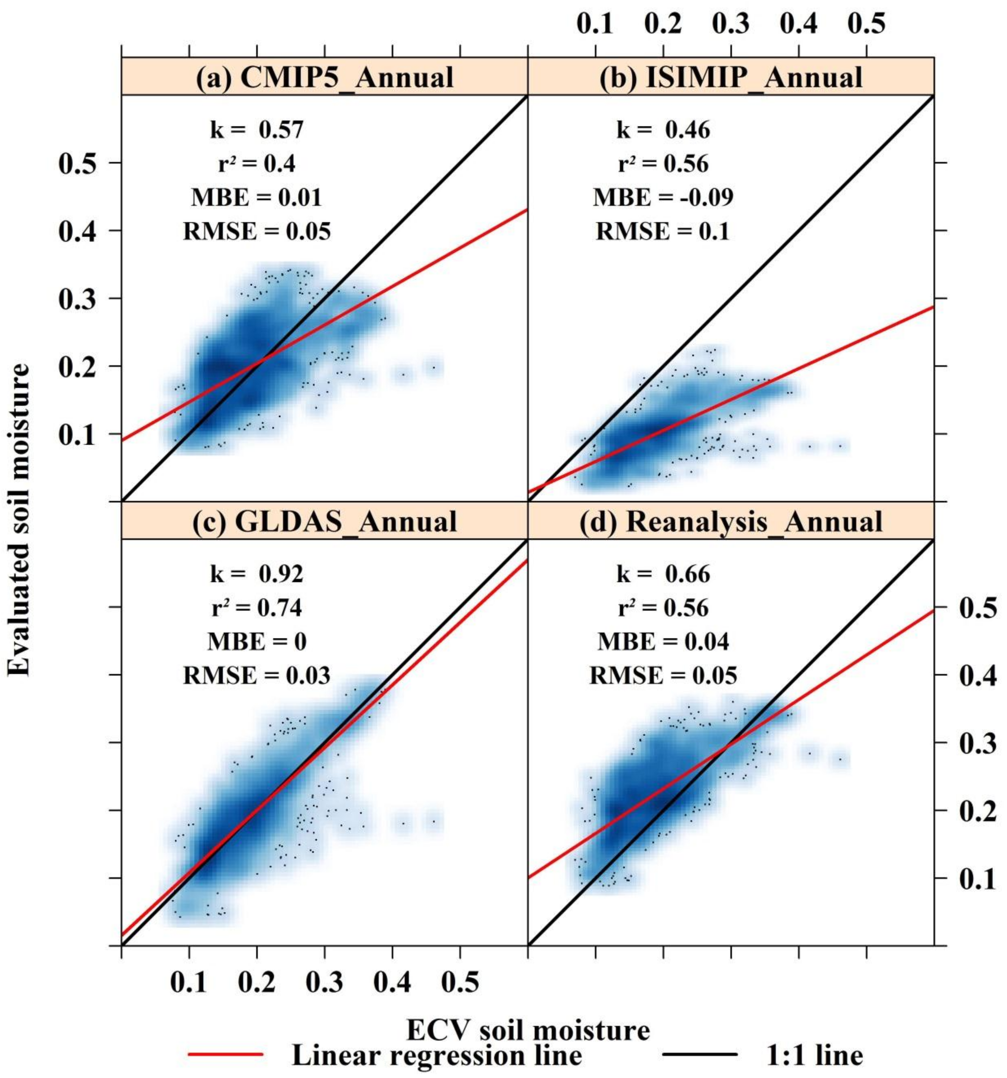
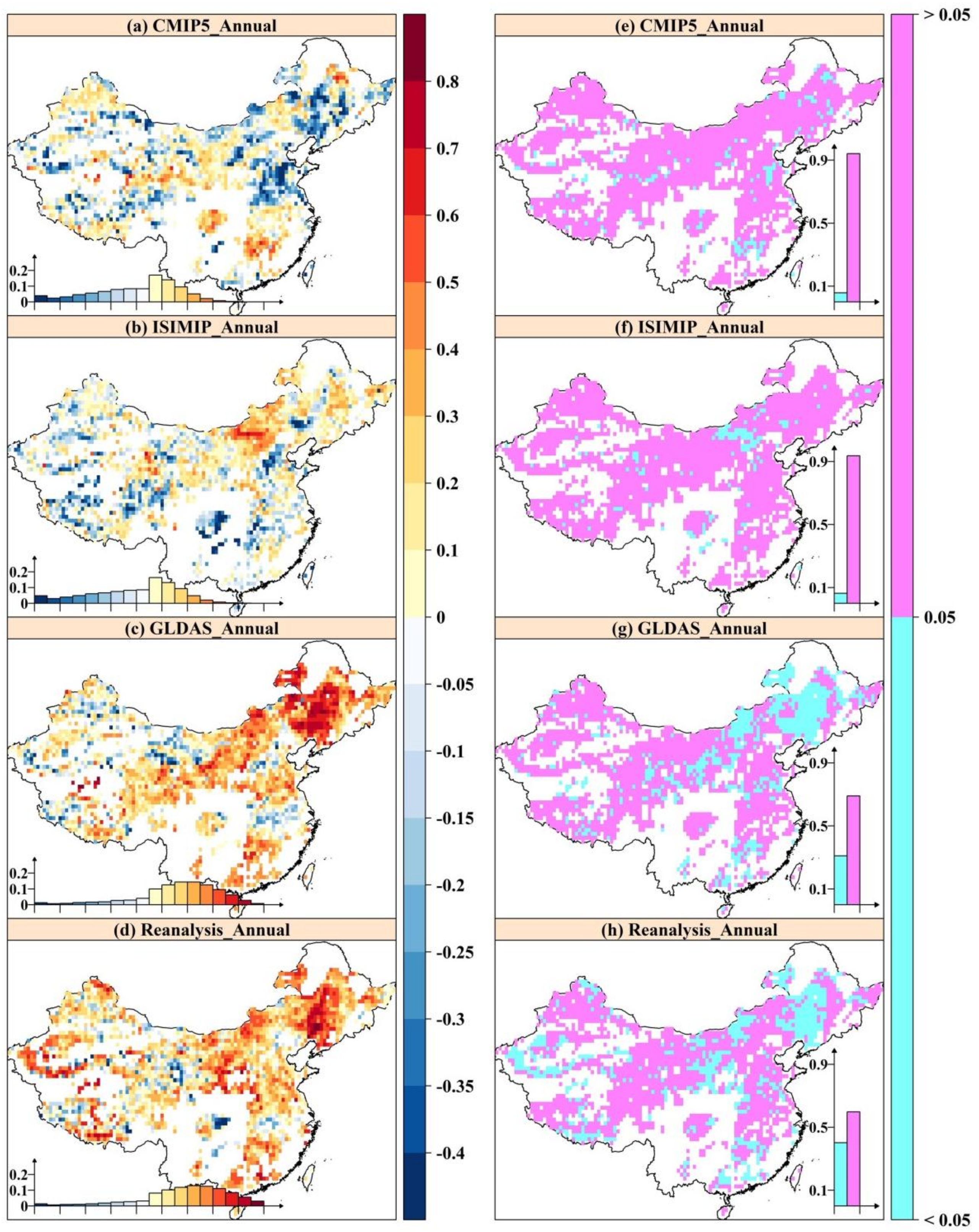
4.1. Comparison of Spatial Patterns of Annual Mean Soil Moisture

The spatial patterns of annual mean soil moisture across China, generated from different ensemble mean datasets (i.e., ECV, CMIP5, ISIMIP, GLDAS, and Reanalysis) from 1980 to 2005, were detected and are presented in Figure 3. The annual mean soil moisture shows gradual increases from northwest to southeast China. The increase is more remarkable in the ECV dataset (Figure 3). All of the ECV and model simulations demonstrate southern China having the wettest soil. The results are in line with those shown by Chen [30] and Cheng [18], and are also in accordance with the spatial pattern of annual mean precipitation. This indicates that both ECV and model simulations are efficient in demonstrating the spatial distribution of soil moisture affected by precipitation. However, the magnitudes of annual mean soil moisture have obvious differences among datasets. The values from ISIMIP are generally smaller than those from the other datasets. On the contrary, Reanalysis shows the highest values among all datasets.
Specifically, annual mean soil moisture in CMIP5 is higher in south China and lower in northwest China, which is in line with ECV. However, CMIP5 shows that northeast China is wetter than the surrounding areas. The lowest values presented by the ISIMIP ensemble means are even obvious in dry areas, i.e., northwest China. Even though ISIMIP soil moisture is generated by hydrological models driven by the bias-corrected CMIP5 meteorological outputs, the values of ISIMIP are obviously smaller than those of CMIP5. The significant underestimation in ISIMIP soil moisture may be induced by the hydrological models. Meanwhile, not considering the land–atmosphere interaction is also a reason for this underestimation. GLDAS has the best agreement with ECV, but some slightly higher values can be detected in the central area of the Tarim Basin in northwest China. In spite of the significant overestimations in other areas, Reanalysis performs better in south China in terms of annual mean soil moisture.
Each type of soil moisture dataset includes a number of outputs (e.g., the CMIP5 dataset includes 37 GCM outputs). The bar chart in the left bottom of each panel indicates how the soil moisture varies among different outputs in the same type of dataset (Figure 3). The ratio of standard deviation to mean of the corresponding ensemble members is considered to evaluate the differences among the outputs in the same type of dataset. A lower ratio means smaller differences among the outputs. GLDAS datasets have the best agreement of soil moisture among the outputs of GLDAS. These ratios of the GLDAS dataset are all smaller than 40%, and most of them are smaller than 30%. Reanalysis datasets also show a better agreement among their three kinds of datasets. However, the CMIP5 and ISIMIP present higher ratios than do GLDAS and Reanalysis. Due to the large uncertainties in the outputs of GCMs, the ratios of the CMIP5 datasets are highest.
The smooth scatterplots visually reveal whether the model simulations systematically underestimate or overestimate soil moisture in comparison with ECV (Figure 4). The CMIP5 and ISIMIP ensemble means have obviously smaller coefficients of linear regression (0.57 and 0.46, respectively) when compared with ECV. Specifically, ISIMIP has the lowest consistency with ECV. The coefficient of linear regression between GLDAS and ECV is 0.92, which is largest among all datasets. The soil moisture ensemble mean of the Reanalysis datasets is generally larger than ECV, indicating that Reanalysis datasets may systematically overestimate soil moisture values.
Taylor diagrams can quantitatively evaluate the statistical performance of model simulations relative to ECV observations in China (Figure 5). The Pearson correlation coefficients of annual and seasonal mean soil moisture between model simulations and ECV are mostly larger than 0.6, suggesting that ECV and model simulations have good consistency in terms of the spatial pattern of soil moisture. Among the model simulation datasets, the GLDAS ensemble mean has the smallest values in these statistics, while ISIMIP has the largest values. The ensemble means of CMIP5 and Reanalysis have relatively similar values in the statistics. For multiple outputs of datasets including CMIP5 and ISIMIP, the statistics of individual outputs in each type of dataset were also compared. A high similarity among these individual outputs can be observed in ISIMIP, GLDAS, and Reanalysis, while a large difference is shown in the outputs of CMIP5. The statistics of CMIP5 outputs have the largest and smallest values of MAE, MBE, RMSE, and unRMSE concurrently. The significant differences among outputs of the same type of dataset demonstrate that multimodel ensembles are necessary to effectively reduce model discrepancies. In terms of unRMSE, all datasets show comparable performances relative to ECV, indicating that all datasets have certain ability to represent soil moisture after removing bias errors.

4.2. Comparison of Soil Moisture Time Series in the Datasets

The annual soil moisture time series between ECV and other datasets were compared in each grid. The MBE was selected as the statistical metric because it could better reflect the difference between ECV and model simulation datasets, i.e., overestimation or underestimation (Figure 6). The histogram of the MBE distribution in each panel indicates pronounced differences among these datasets. The MBE values in GLDAS range from −0.02 to 0.02 in most areas of China. The negative values are mainly distributed in western China, while positive values are in eastern China. The significant underestimations in ISIMIP are detected over all areas where most of the MBE values are negative. About 50% of areas of China show MBE values smaller than −0.1, mainly concentrated in the Tibetan Plateau and south China. On the contrary, CMIP5 and Reanalysis datasets show positive MBE values in most areas, especially Reanalysis. CMIP5 mainly manifests in overestimations with MBE values greater than 0.08. These overestimated areas are mainly distributed in northern China and the east parts of the Tibetan Plateau. Similar to CMIP5, Reanalysis datasets also present overestimations in parts of northwestern China. The overestimations in Reanalysis datasets relative to ECV in northwestern China may be associated with the composition of soil moisture, i.e., liquid and solid water. Reanalysis datasets include both liquid and solid water while the ECV only reflects the liquid water [35]. Thus, Reanalysis values are assessed to be higher than those of ECV during the frozen season.
The spatial patterns of RMSE and unRMSE were estimated from the annual soil moisture of modeled datasets relative to the ECV (Figure 7). The spatial distribution of RMSE in ISIMIP shows the highest RMSE values on the Tibetan Plateau and in the south regions (RMSE > 0.125). The higher values of RMSE in CMIP5 and Reanalysis datasets are shown in the east of the Tibetan Plateau and northwest China. In addition, the RMSE values in CMIP5 are also higher in the marginal parts of the north and south China, while the RMSE in Reanalysis is higher in both the east and west margins of northwest China. The spatial distribution of RMSE is significantly different in GLDAS, where it is distributed uniformly in spatial patterns.
Unlike the significant difference in RMSE, the spatial pattern of unRMSE in the modeled datasets is more uniform. The similar spatial pattern of unRMSE further indicates that the random errors of modeled datasets relative to the ECV are similar after removing the bias errors. The smaller magnitude unRMSE (<0.01) of the modeled datasets is mainly concentrated in northwest China. ECV was scaled by the GLDAS-Noah surface soil moisture product, leading to the lowest values in RMSE between GLDAS and ECV. Additionally, after removing the bias errors, the large differences in RMSE between model simulations and ECV are reduced obviously. Comparing the results of RMSE and unRMSE, the deviations between the ECV and modeled datasets are caused by the bias errors.
Therefore, the anomalies in annual soil moisture were used to calculate the Pearson correlation coefficient to remove the impacts of absolute means (Figure 8). The equation z = ( x i μ ) / σ was used to normalize the annual soil moisture dataset, and the period of 1980–2005 was used as the reference period. In the equation, x i is the annual soil moisture value of the ith year, μ is the mean for the whole series, and σ is the standard deviation for the whole series [80]. The spatial patterns of the Pearson correlation coefficient of soil moisture anomalies were different among datasets. Weaker correlations were detected in CMIP5 and ISIMIP compared with GLDAS and Reanalysis. Moreover, negative correlations were detected in quite a few areas by CMIP5 and ISIMIP (Figure 8a,b), and more than 90% of these areas were statistically insignificant (Figure 8e,f). However, positive correlations of GLDAS and Reanalysis datasets could be detected in almost all areas, and about half of these areas presented statistical significance (Figure 8g,h). The areas with statistically positive correlations were mainly distributed in northern China where correlation coefficients were more than 0.8.

4.3. Comparison of Long-Term Seasonal Trends of the Soil Moisture Datasets

The Sen’s slopes of annual soil moisture in ECV, ISIMIP, GLDAS, and Reanalysis show drying trends in more than 50% of the areas, except for CMIP5 (Figure 9 and Figure S1). The overall drying trends were also detected and verified over East Asia based on GLDAS-2 datasets over a period of 63 years during 1948–2010 [18]. The percentages of significant drying trends in GLDAS and Reanalysis are 41% and 32%, respectively, which are pronouncedly higher than in the other datasets (Figure 8d,e). Even though the percentages of significant drying trends in ECV and ISIMIP are much lower, the consensus of a drying trend is clearly detected. However, the regional trends are different in various regions. For example, the drying trends in northwest and north China were detected by most of the datasets except for CMIP5, which shows a pronounced wetting trend in this region. This inconsistency of the trend among different datasets was also detected in south China. In this region, the overall drying trend was detected by the modeled datasets except for the ECV, which shows a pronounced wetting trend, especially in the southeast region. Additionally, this wetting trend was also detected by ECV during 2003–2010 in eastern China by An et al. [37] while significant drying trends were detected in eastern China during 1979–2010 based on ECV [30]. This reflects the variability in long-term drying of soil moisture. Overall, the results of Sen’s slopes in the Tibetan Plateau are more divergent because of the complexity of the environment. Previous studies also suggested that the complexity of the land surface environment would increase the uncertainty of the model simulation [8].
Both precipitation and NDVI are sensitive to the seasonal variation of soil moisture [28]. To validate whether the spatial patterns of trends in soil moisture were reasonable, the trends of annual and seasonal precipitation and NDVI were detected (Figure 10). The trends of precipitation and NDVI seem to support the wetting trend patterns in ECV and CMIP5 (Figure 9 and Figure S1). For example, the wetting trends of soil moisture in ECV and CMIP5 are found in some parts of north and northwest China, and the trends are consistent with the increasing precipitation and NDVI in these areas. However, this phenomenon contradicts the drying trends in other datasets, especially GLDAS. On the other hand, the most drying trends in soil moisture are supported by a decrease in precipitation, such as in the northern parts of north China. However, the drying trends in south China detected in soil moisture and precipitation datasets are not reflected by NDVI. This inconsistent phenomenon between precipitation and NDVI is prominent in the summer. The precipitation in the south China generally presents decreasing trends in summer and increasing trends in autumn. However, the NDVI in these areas presents increasing trends almost all the year. These results indicate that the trends in surface soil moisture are more consistent with the changes in precipitation than those in NDVI. The reasons for this are likely that most modeled datasets are driven by precipitation. Further, it is difficult to fully consider the complex land–atmosphere interactions and ecosystem responses in most model simulations [39].
The spatial distributions of the Sen’s slopes for soil moisture are more consistent with precipitation, as shown in Figure 9 and Figure 10 and Figure S1. To identify the impacts of the seasonal precipitation, the Sen’s slopes of soil moisture (including ECV, CMIP5, ISIMIP GLDAS, and Reanalysis) were further detected. The Sen’s slopes of soil moisture in different datasets have the same trend directions with those of precipitation, and the spatial distributions of each grid are shown in Figure 11. Overall, the agreement of drying trends between precipitation and soil moisture of GLDAS and Reanalysis datasets was more evident than the agreements of the ECV, CMIP5, and ISIMIP. These agreements between precipitation and soil moisture of the GLDAS and Reanalysis datasets at annual and seasonal scales were found in south China and some parts of north China.
The agreements between precipitation and soil moisture in GLDAS and Reanalysis datasets at annual and seasonal scales are pronounced in autumn. However, these agreements are poor in summer. These poor agreements can be remedied by ECV and CMIP5 to some extent, especially by ECV. Further, past studies indicated that surface soil moisture variations were mainly driven by precipitation, especially in areas with a moisture-limited evaporation mechanism [4]. The high sensitivity of soil moisture variations to precipitation can be captured in CMIP5 in northwest China where slight increases in precipitation in winter and spring cause significant soil moisture wetting [61]. In winter, good agreements between precipitation and soil moisture can be observed in GLDAS in the eastern area of south China, followed by Reanalysis. Overall, the distribution patterns of soil moisture vary in different regions and seasons.

5. Conclusions

In this study, five soil moisture datasets—an ECV remote sensing dataset and CMIP5, ISIMIP, GLDAS, and Reanalysis datasets—were compared to understand the similarities and differences of these datasets for climate change studies. The surface soil moisture over a period of 26 years was compared to evaluate the long-term performances among these datasets in China.
All datasets show a spatial pattern of “southeast, wettest and northwest, driest” in soil moisture. The ECV remote sensing dataset effectively shows the spatial pattern of soil moisture and its potential for evaluating model simulation performance. When compared to ECV, GLDAS has the best performance among the modeled datasets, especially in north, northwest China and the Tibetan Plateau. Reanalysis also performs better in north and northwest China. In spite of the significant underestimations in soil moisture, ISIMIP performs better in northwest China in terms of annual mean soil moisture. CMIP5 can successfully represent the spatial pattern of soil moisture, but it has considerable discrepancies in local areas.
The Pearson correlation coefficients of annual mean soil moisture between the model simulation ensemble and ECV are mostly larger than 0.6. The results indicate that these datasets have a good consensus on the spatial correlations. Nevertheless, the differences in RMSE and unRMSE between ECV and model simulations indicate that the bias errors and random errors are obvious among these datasets. There are considerable discrepancies in the absolute values of soil moisture among these datasets produced by different techniques. After removing the differences in absolute values, the discrepancies of these datasets are mitigated. On the other hand, the outputs in the same type of dataset also present pronounced discrepancies. The outputs of GLDAS have the best consistency with each other, followed by Reanalysis with three outputs. The outputs of the CMIP5 (37 individual outputs) and ISIMIP (14 individual outputs) manifest larger differences, especially CMIP5.
Precipitation is a major factor that influences soil moisture variations, and NDVI is sensitive to soil moisture changes. Therefore, precipitation and NDVI can be used to validate which dataset can show more reasonable trends in soil moisture. In spring, CMIP5 in northwest China shows trends in soil moisture consistent with the changes in precipitation and NDVI. In summer, ECV presents the most identical performance compared to the changes in precipitation and NDVI. In autumn, GLDAS and Reanalysis have better performance in south China and parts of north China. In winter, GLDAS has the best performance in the east of south China, followed by the Reanalysis dataset.

6. Discussion

The discrepancies among these datasets are apparent in specific geographical zones. Therefore, it is very necessary to discuss the possible reasons behind these discrepancies and the factors contributing to these discrepancies. Considering the formats of these datasets, one possible reason is that the layer depths are different. The layer depths among different datasets vary in a range between 0.02 m and 0.5 m (Table 1, Table 2, Table 3, Table 4 and Table 5), especially between the simulations and the remote sensing datasets. In our study, the closest layers to the surface were selected uniformly. However, we could not avoid the risk of introducing further difference into the results from their diverse layer depths. In particular, the largest deviation in layer depths between ECV and ISIMIP datasets possibly led to the largest absolute deviations in the soil moisture value. Therefore, multiple statistical metrics were compared among different datasets to eliminate the possible uncertainty of different layer depths. Another reason is the difference in spatial resolutions among different datasets. In our study, the spatial resolutions of different datasets are normalized to the 0.5° × 0.5° resolution by a bilinear interpolation method. The preprocessing may introduce new uncertain impacts on the final results.
Moreover, considering the datasets generated by models, some factors including model structure, model parameters, and forcing data should also be influential. These factors can introduce uncertainties into model-simulated soil moisture [35,39]. For example, ISIMIP datasets are outputs of different hydrological models forced by different GCMs. Among the 30 outputs of ISIMIP datasets, the outputs present vast differences. Additionally, the LSMs forced in GLDAS have different parameters, which also leads to different performances in terms of soil moisture. Soil texture data may also influence parameters in land surface models (LSMs) in GLDAS datasets, i.e., Community Land Model/CLM, Mosaic/MOS, Variable Infiltration Capacity/VIC, and Noah/NOAH. All LSMs in GLDAS use the same soil texture data to simulate soil moisture; hence, the errors in soil texture propagated to soil moisture products may be negligible. The soil texture was derived from the global soils dataset by Reynolds, Jackson, and Rawls, and includes fractions of sand, silt, and clay, and porosity, among other fields, based on the FAO Soil Map (Figure S2). However, the resampling of the soil texture to satisfy the layer depth of different LSMs may have influences on soil moisture products [83,84,85,86]. In our paper, only soil moisture in the top layer of depth of LSMs was used, which may reduce the influences.
In addition, irrigation also plays an important role in soil moisture changes. Satellite observations (i.e., the ECV dataset) can reflect the influences of irrigation on soil moisture, while model simulations do not consider the irrigation components. The Huang-Huai-Hai Plain is the most intensively irrigated area in China. A recent report by Qiu et al. [42] found that the ECV dataset could capture soil moisture changes more accurately than model simulations and pointed out that it was crucial for models to consider irrigation in areas with a great magnitude of human interference in order to successfully simulate soil moisture. We also observed the disagreements in derived trends between ESA CCI and model-simulated datasets in the Huang-Huai-Hai Plain. The intensive irrigation is considered to be the underlying cause for the discrepancy in soil moisture trends at regional scale, because irrigation as an additional water supply source has the impact of reducing soil albedo, increasing soil heat capacity, altering local soil moisture content, and affecting the water/energy budget by transforming the evapotranspiration regime from water-limited to energy-limited [42,87,88,89].
The ECV datasets are also significantly influenced by many factors, such as different sensors, Radio Frequency Interference (RFI), retrieval algorithm, land conditions, and weather [31,35,58]. These discrepancies among the datasets result in various changes in different regions. The limitations and uncertainties of soil moisture datasets also change by season. These limitations and uncertainties of the different datasets should be well noted and discussed before use. Our results will be valuable to improving the understanding of the similarities and differences of different soil moisture datasets. Thus, the results of this paper will provide scientific support to climate studies based on different soil moisture datasets.

Supplementary Materials

The following are available online at https://www.mdpi.com/2073-4441/10/10/1384/s1, Figure S1: Spatial distributions of P-value of Sen’s slope of annual soil moisture in ECA, GLDAS, Reanalysis, CMIP5, and ISIMIP, Figure S2 Spatial distributions of soil texture used in GLDAS LSMs.

Author Contributions

Conceptualization, W.B. and X.H.G.; Methodology, W.B. and X.H.G.; Software, W.B and X.L.G.; Formal Analysis, W.B. and X.H.G.; Investigation, W.B. and X.L.G.; Writing-Original Draft Preparation, W.B.; Writing-Review & Editing, W.B., S.L., Y.T., X.H.G., Y.H. and X.B. All authors read and approved the final manuscript.

Funding

This research was funded by the National Key Research and Development Program of China (Grant No. 2018YFA0605603), the Strategic Priority Research Program Grant of the Chinese Academy of Sciences (Grant No. XDA19070402), the Fundamental Research Funds for the Central Universities, China University of Geosciences (Wuhan) (Grant No. CUG180614 and CUGCJ1702), a grant from the Research Grants Council of the Hong Kong Special Administrative Region, China (Project No. HKBU22301916), the National Natural Science Foundation of China (Grant No. 91547202, 51479216, 51509127 and 51509040), and National Key R&D Program of China (2017YFC0405900).

Acknowledgments

We would like to thank all study participants for the participation and the three famous reviewers.

Conflicts of Interest

The authors declare no conflict of interest.

References

  1. Srinivasan, G.; Robock, A.; Entin, J.K.; Luo, L.; Vinnikov, K.Y.; Viterbo, P. Soil moisture simulations in revised amip models. J. Geophys. Res. Atmos. 2000, 105, 26635–26644. [Google Scholar] [CrossRef]
  2. Koster, R.D.; Yamada, T. Regions of strong coupling between soil moisture and precipitation. Science 2004, 305, 1138–1140. [Google Scholar] [CrossRef] [PubMed]
  3. Fischer, E.M.; Seneviratne, S.I.; Vidale, P.L.; Lüthi, D.; Schär, C. Soil moisture atmosphere interactions during the 2003 european summer heat wave. J. Clim. 2007, 20, 5081. [Google Scholar] [CrossRef]
  4. Jung, M.; Reichstein, M.; Ciais, P.; Seneviratne, S.I.; Sheffield, J.; Goulden, M.L.; et al. Recent decline in the global land evapotranspiration trend due to limited moisture supply. Nature 2010, 467, 951–954. [Google Scholar] [CrossRef] [PubMed] [Green Version]
  5. Amani, M.; Salehi, B.; Mahdavi, S.; Masjedi, A.; Dehnavi, S. Temperature-Vegetation-soil Moisture Dryness Index (TVMDI). Remote Sens. Environ. 2017, 197, 1–14. [Google Scholar] [CrossRef]
  6. Seneviratne, S.I.; Corti, T.; Davin, E.L.; Hirschi, M.; Jaeger, E.B.; Lehner, I.; Bonan, G.; Cescatti, A.; Chen, J.; de Jeu, R.; et al. Investigating soil moisture–climate interactions in a changing climate: A review. Earth-Sci. Rev. 2010, 99, 125–161. [Google Scholar] [CrossRef]
  7. Li, H.; Shen, W.; Zou, C.; Jiang, J.; Fu, L.; She, G. Spatio-temporal variability of soil moisture and its effect on vegetation in a desertified aeolian riparian ecotone on the tibetan plateau, China. J. Hydrol. 2013, 479, 215–225. [Google Scholar] [CrossRef]
  8. Bi, H.; Ma, J.; Zheng, W.; Zeng, J. Comparison of soil moisture in GLDAS model simulations and in situ observations over the Tibetan Plateau. J. Geophys. Res. Atmos. 2016, 121, 2658–2678. [Google Scholar] [CrossRef]
  9. Albergel, C.; de Rosnay, P.; Gruhier, C.; Muñoz-Sabater, J.; Hasenauer, S.; Isaksen, L.; Kerr, Y.; Wagner, W. Evaluation of remotely sensed and modelled soil moisture products using global ground-based in situ observations. Remote Sens. Environ. 2012, 118, 215–226. [Google Scholar] [CrossRef]
  10. Yang, K. A multi-scale soil moisture and freeze-thaw monitoring network on the tibetan plateau and its applications. Bull. Am. Meteorol. Soc. 2013, 94, 1907–1916. [Google Scholar] [CrossRef]
  11. Gao, Z.; Chae, N.; Kim, J.; Hong, J.; Choi, T.; Lee, H. Modeling of surface energy partitioning, surface temperature, and soil wetness in the tibetan prairie using the simple biosphere model 2 (sib2). J. Geophys. Res. Atmos. 2004, 109, 439–447. [Google Scholar] [CrossRef]
  12. Yang, Z.; Hua, O.; Zhang, X.; Xu, X.; Zhou, C.; Yang, W. Spatial variability of soil moisture at typical alpine meadow and steppe sites in the qinghai-tibetan plateau permafrost region. Environ. Earth Sci. 2011, 63, 477–488. [Google Scholar] [CrossRef]
  13. Zhang, X.F.; Zhao, L.; Xu, S.J.; Liu, Y.Z.; Liu, H.Y.; Cheng, G.D. The influence of soil moisture on bacterial and fungal communities in beilu river (tibetan plateau) permafrost soils with different vegetation types. J. Appl. Microbiol. 2012, 114, 1054–1065. [Google Scholar] [CrossRef] [PubMed]
  14. Taylor, C.M.; de Jeu, R.A.; Guichard, F.; Harris, P.P.; Dorigo, W.A. Afternoon rain more likely over drier soils. Nature 2012, 489, 423. [Google Scholar] [CrossRef] [PubMed] [Green Version]
  15. Cheng, S.; Huang, J.; Li, F.; Lin, L. Uncertainties of soil moisture in historical simulations and future projections. J. Geophys. Res. Atmos. 2017, 122, 2239–2253. [Google Scholar] [CrossRef]
  16. Ruosteenoja, K.; Markkanen, T.; Venäläinen, A.; Räisänen, P.; Peltola, H. Seasonal soil moisture and drought occurrence in europe in cmip5 projections for the 21st century. Clim. Dyn. 2017, 50, 1–16. [Google Scholar] [CrossRef]
  17. Zhao, L.; Yang, K.; Qin, J.; Chen, Y.; Tang, W.; Montzka, C.; Wu, H.; Lin, C.; Han, M.; Vereecken, H. Spatiotemporal analysis of soil moisture observations within a tibetan mesoscale area and its implication to regional soil moisture measurements. J. Hydrol. 2013, 482, 92–104. [Google Scholar] [CrossRef]
  18. Cheng, S.; Guan, X.; Huang, J.; Ji, F.; Guo, R. Long-term trend and variability of soil moisture over East Asia. J. Geophys. Res. Atmos. 2015, 120, 8658–8670. [Google Scholar] [CrossRef]
  19. Ochsner, T.E.; Cosh, M.H.; Cuenca, R.H.; Dorigo, W.A.; Draper, C.S.; Hagimoto, Y.; Kerr, Y.H.; Njoku, E.G.; Smali, E.E.; Zreda, M. State of the art in large-scale soil moisture monitoring. Soil Sci. Soc. Am. J. 2013, 77, 1888–1919. [Google Scholar] [CrossRef] [Green Version]
  20. Brocca, L.; Hasenauer, S.; Lacava, T.; Melone, F.; Moramarco, T.; Wagner, W.; Dorigo, W.; Matgen, P.; Martínez-Fernándeze, J.; Llorensf, P.; et al. Soil moisture estimation through ASCAT and AMSR-E sensors: An intercomparison and validation study across Erope. Remote Sens. Environ. 2011, 115, 3390–3408. [Google Scholar] [CrossRef]
  21. Koike, T.; Nakamura, Y.; Kaihotsu, I.; Davaa, G.; Matsuura, N.; Tamagawa, K.; Fujii, H. Development of an advanced microwave scanning radiometer (AMSR-E) algorithm for soil moisture and vegetation water content. Doboku Gakkai Ronbunshuu B 2004, 48, 217–222. [Google Scholar] [CrossRef]
  22. Kerr, Y.H.; Waldteufel, P.; Wigneron, J.P.; Delwart, S.; Cabot, F.O.; Boutin, J.; Escorihuela, M.-J.; Font, J.; Reul, N.; Gruhier, C.; et al. The SMOS mission: New tool for monitoring key elements of the global water cycle. Proc. IEEE. 2010, 98, 666–687. [Google Scholar] [CrossRef] [Green Version]
  23. Kerr, Y.H.; Waldteufel, P.; Richaume, P.; Wigneron, J.P.; Ferrazzoli, P.; Mahmoodi, A.; Bitar, A.A.; Cabot, F.; Gruhier, C.; Jugleat, S.E.; et al. The smos soil moisture retrieval algorithm. IEEE Trans. Geosci. Remote 2012, 50, 1384–1403. [Google Scholar] [CrossRef]
  24. Njoku, E.G.; Chan, S.K. Vegetation and surface roughness effects on AMSR-E land observations. Remote Sens. Environ. 2006, 100, 190–199. [Google Scholar] [CrossRef]
  25. Naeimi, V.; Scipal, K.; Bartalis, Z.; Hasenauer, S.; Wagner, W. An improved soil moisture retrieval algorithm for ers and metop scatterometer observations. IEEE Trans. Geosci. Remote 2009, 47, 1999–2013. [Google Scholar] [CrossRef]
  26. Entekhabi, D.; Njoku, E.G.; Neill, P.E.; Kellogg, K.H.; Crow, W.T.; Edelstein, W.N.; Entin, J.K.; Goodman, S.D.; Jackson, T.J.; Johnson, J.; et al. The soil moisture active passive (SMAP) mission. Proc. IEEE 2010, 98, 704–716. [Google Scholar] [CrossRef]
  27. Owe, M.; Jeu, R.D.; Holmes, T. Multisensor historical climatology of satellite-derived global land surface moisture. J. Geophys. Res.-Earth Surf. 2008, 113, 1–17. [Google Scholar] [CrossRef]
  28. Dorigo, W.; Jeu, R.D.; Chung, D.; Parinussa, R.; Liu, Y.; Wagner, W.; Fernández-Prieto, D. Evaluating global trends (1988–2010) in harmonized multi-satellite surface soil moisture. Geophys. Res. Lett. 2012, 39, 18405. [Google Scholar] [CrossRef]
  29. Parinussa, R.; Meesters, A.G.C.A.; Liu, Y.Y.; Dorigo, W.; Wagner, W.; De Jeu, R.A.M. An analytical solution to estimate the error structure of a global soil moisture dataset. IEEE Geosci. Remote Sens. Lett. 2011, 8, 779–783. [Google Scholar] [CrossRef]
  30. Chen, X.; Su, Y.; Liao, J.; Shang, J.; Dong, T.; Wang, C.; Liu, W.; Zhou, G.; Liu, L. Detecting significant decreasing trends of land surface soil moisture in eastern China during the past three decades (1979–2010). J. Geophys. Res. Atmos. 2016, 121, 5177–5192. [Google Scholar] [CrossRef]
  31. Dorigo, W.A.; Gruber, A.; Jeu, R.A.M.D.; Wagner, W.; Stacke, T.; Loew, A.; Albergel, C.; Brocca, L.; Chung, D.; Parinussa, R.M.; et al. Evaluation of the ESA CCI soil moisture product using ground-based observations. Remote Sens. Environ. 2015, 162, 380–395. [Google Scholar] [CrossRef]
  32. Feng, H. Individual contributions of climate and vegetation change to soil moisture trends across multiple spatial scales. Sci. Rep. 2016, 6, 32728. [Google Scholar] [CrossRef] [PubMed]
  33. Liu, Y.Y.; Parinussa, R.M.; Dorigo, W.A.; De Jeu, R.A.M.; Wagner, W.; van Dijk, A.I.J.M.; McCabe, M.F.; Evans, J.P. Developing an improved soil moisture dataset by blending passive and active microwave satellite-based retrievals. Hydrol. Earth Syst. Sci. 2011, 15, 425–436. [Google Scholar] [CrossRef] [Green Version]
  34. Liu, Y.Y.; Dorigo, W.A.; Parinussa, R.M.; De Jeu, R.A.M.; Wagner, W.; McCabe, M.F.; Evans, J.P.; van Dijk, A.I.J.M. Trend-preserving blending of passive and active microwave soil moisture retrievals. Remote Sens. Environ. 2012, 123, 280–297. [Google Scholar] [CrossRef]
  35. Zeng, J.; Li, Z.; Chen, Q.; Bi, H.; Qiu, J.; Zou, P. Evaluation of remotely sensed and reanalysis soil moisture products over the tibetan plateau using in-situ observations. Remote Sens. Environ. 2015, 163, 91–110. [Google Scholar] [CrossRef]
  36. Nicolai-Shaw, N.; Hirschi, M.; Mittelbach, H.; Seneviratne, S.I. Spatial representativeness of soil moisture using in situ, remote sensing, and land reanalysis data. J. Geophys. Res. Atmos. 2015, 120, 9955–9964. [Google Scholar] [CrossRef] [Green Version]
  37. An, R.; Zhang, L.; Wang, Z.; Quaye-Ballard, J.A.; You, J.; Shen, X.; Gao, W.; Huang, L.; Zhao, Y.; Ke, Z. Validation of the esa cci soil moisture product in China. Int. J. Appl. Earth Obs. Geoinf. 2016, 48, 28–36. [Google Scholar] [CrossRef]
  38. Jing, W.; Song, J.; Zhao, X. A comparison of ecv and smos soil moisture products based on oznet monitoring network. Remote Sens. 2018, 10, 703. [Google Scholar] [CrossRef]
  39. Yuan, S.; Quiring, S.M. Evaluation of soil moisture in CMIP5 simulations over the contiguous United States using in situ and satellite observations. Hydrol. Earth Syst. Sci. 2017, 21, 2203–2218. [Google Scholar] [CrossRef] [Green Version]
  40. Loew, A.; Stacke, T.; Dorigo, W.; de Jeu, R.; Hagemann, S. Potential and limitations of multidecadal satellite soil moisture observations for selected climate model evaluation studies. Hydrol. Earth Syst. Sci. 2013, 17, 3523–3542. [Google Scholar] [CrossRef] [Green Version]
  41. Feng, H.; Zhang, M. Global land moisture trends: Drier in dry and wetter in wet over land. Sci. Rep. 2015, 5. [Google Scholar] [CrossRef] [PubMed]
  42. Qiu, J.; Gao, Q.; Wang, S.; Su, Z. Comparison of temporal trends from multiple soil moisture data sets and precipitation: The implication of irrigation on regional soil moisture trend. Int. J. Appl. Earth Obs. Geoinf. 2016, 48, 17–27. [Google Scholar] [CrossRef] [Green Version]
  43. Dorigo, W.; Wagner, W.; Albergel, C.; Albrecht, F.; Balsamo, G.; Brocca, L.; Chung, D.; Ertl, M.; Forkel, M.; Gruber, A.; et al. ESA CCI soil moisture for improved earth system understanding: State-of-the art and future directions. Remote Sens. Environ. 2017, 203, 185–215. [Google Scholar] [CrossRef]
  44. Szczypta, C.; Calvet, J.C.; Maignan, F.; Dorigo, W.; Baret, F.; Ciais, P. Suitability of modelled and remotely sensed essential climate variables for monitoring Euro-Mediterranean droughts. Geosci. Model Dev. 2014, 7, 931–946. [Google Scholar] [CrossRef] [Green Version]
  45. Reichle, R.H.; Koster, R.D.; Liu, P.; Mahanama, S.P.P.; Njoku, E.G.; Owe, M. Comparison and assimilation of global soil moisture retrievals from the advanced microwave scanning radiometer for the earth observing system (AMSR-E) and the scanning multichannel microwave radiometer (SMMR). J. Geophys. Res. Atmos. 2007, 112. [Google Scholar] [CrossRef]
  46. Van, d.V.R.; Salama, M.S.; Pellarin, T.; Ofwono, M.; Ma, Y.; Su, Z. Long term soil moisture mapping over the tibetan plateau using special sensor microwave/imager. Hydrol. Earth Syst. Sci. 2013, 18, 6629–6667. [Google Scholar]
  47. Zeng, J.; Li, Z.; Chen, Q.; Bi, H. Method for soil moisture and surface temperature estimation in the tibetan plateau using spaceborne radiometer observations. IEEE Geosci. Remote Sens. Lett. 2015, 12, 97–101. [Google Scholar] [CrossRef]
  48. Rodell, M.; Houser, P.R.; Jambor, U.; Gottschalck, J.; Mitchell, K.; Meng, C.-J.; Arsenault, K.; Cosgrove, B.; Radakovich, J.; Bosilovich, M.; et al. The Global Land Data Assimilation System. Bull. Am. Meteorol. Soc. 2004, 85, 381–394. [Google Scholar] [CrossRef] [Green Version]
  49. Taylor, K.E.; Stouffer, R.J.; Meehl, G.A. An overview of CMIP5 and the experiment design. Bull. Am. Meteorol. Soc. 2012, 93, 485–498. [Google Scholar] [CrossRef]
  50. Crow, W.T.; Berg, A.A.; Cosh, M.H.; Loew, A.; Mohanty, B.P.; Panciera, R.; de Rosnay, P.; Ryu, D.; Walker, J.P. Upscaling sparse ground-based soil moisture observations for the validation of coarse-resolution satellite soil moisture products. Rev. Geophys. 2012, 50. [Google Scholar] [CrossRef] [Green Version]
  51. Su, Z.; Wen, J.; Dente, L.; van der Velde, R.; Wang, L.; Ma, Y.; Yang, K.; Hu, Z. The tibetan plateau observatory of plateau scale soil moisture and soil temperature (Tibet-Obs) for quantifying uncertainties in coarse resolution satellite and model products. Hydrol. Earth Syst. Sci. 2011, 15, 2303–2316. [Google Scholar] [CrossRef]
  52. Sillmann, J.; Kharin, V.V.; Zhang, X.; Zwiers, F.W.; Bronaugh, D. Climate extremes indices in the cmip5 multimodel ensemble: Part 1. Model evaluation in the present climate. J. Geophys. Res. Atmos. 2013, 118, 1716–1733. [Google Scholar] [CrossRef]
  53. Sillmann, J.; Kharin, V.V.; Zwiers, F.W.; Zhang, X.; Bronaugh, D. Climate extremes indices in the CMIP5 multimodel ensemble: Part 2. Future climate projections. J. Geophys. Res. Atmos. 2013, 118, 2473–2493. [Google Scholar] [CrossRef] [Green Version]
  54. Warszawski, L.; Frieler, K.; Huber, V.; Piontek, F.; Serdeczny, O.; Schewe, J. The inter-sectoral impact model intercomparison project (ISI–MIP): Project framework. Proc. Natl. Acad. Sci. USA 2014, 111, 3228–3232. [Google Scholar] [CrossRef] [PubMed]
  55. Dee, D.P.; Uppala, S.M.; Simmons, A.J.; Berrisford, P.; Poli, P.; Kobayashi, S.; Andrae, U.; Balmaseda, M.A.; Balsamo, G.; Bauer, P.; et al. The ERA-interim reanalysis: Configuration and performance of the data assimilation system. Q. J. R. Meteorolog. Soc. 2011, 137, 553–597. [Google Scholar] [CrossRef]
  56. Rienecker, M.M.; Suarez, M.J.; Gelaro, R.; Todling, R.; Bacmeister, J.; Liu, E.; Bosilovich, M.G.; Schubert, S.D.; Takacs, L.; Kim, G.-K.; et al. MERRA: NASA’s modern-era retrospective analysis for research and applications. J. Clim. 2011, 24, 3624–3648. [Google Scholar] [CrossRef]
  57. Lau, N.-C.; Nath, M.J. Model simulation and projection of European heat waves in present-day and future climates. J. Clim. 2014, 27, 3713–3730. [Google Scholar] [CrossRef]
  58. Ferguson, C.R.; Wood, E.F. Observed land-atmosphere coupling from satellite remote sensing and reanalysis. J. Hydrometeorol. 2011, 12, 1221–1254. [Google Scholar] [CrossRef]
  59. Albergel, C.; Dorigo, W.; Balsamo, G.; Muñoz-Sabater, J.; Rosnay, P.D.; Isaksen, L.; Brocca, L.; de Jeu, R.; Wagner, W. Monitoring multi-decadal satellite earth observation of soil moisture products through land surface reanalyses. Remote Sens. Environ. 2013, 138, 77–89. [Google Scholar] [CrossRef]
  60. Bitar, A.A.; Leroux, D.; Kerr, Y.H.; Merlin, O.; Richaume, P.; Sahoo, A.; Wood, E.F. Evaluation of smos soil moisture products over continental U.S. using the SCAN/SNOTEL network. IEEE Trans. Geosci. Remote 2012, 50, 1572–1586. [Google Scholar] [CrossRef] [Green Version]
  61. Qin, D.; Tao, S.; Dong, S.; Luo, Y. Climate, Environmental, and Socioeconomic Characteristics of China. In Climate and Environmental Change in China: 1951–2012; Springer: Berlin/Heidelberg, Germany, 2016. [Google Scholar]
  62. He, Y. China’s geographical regionalization in Chinese secondary school curriculum (1902–2012). J. Geogr. Sci. 2013, 23, 370–383. [Google Scholar] [CrossRef]
  63. Berg, A.; Lintner, B.R.; Findell, K.; Giannini, A. Uncertain soil moisture feedbacks in model projections of Sahel precipitation. Geophys. Res. Lett. 2017, 44, 6124–6133. [Google Scholar] [CrossRef]
  64. Tang, Q.; Oki, T.; Kanae, S. A distributed biosphere hydrological model (DBHM) for large river basin. Proc. Hydraul. Eng. 2006, 50, 37–42. [Google Scholar] [CrossRef]
  65. Tang, Q.; Oki, T.; Kanae, S.; Hu, H. The influence of precipitation variability and partial irrigation within grid cells on a hydrological simulation. J. Hydrometeorol. 2007, 8, 499–512. [Google Scholar] [CrossRef]
  66. Bierkens, M.F.P.; van Beek, L.P.H. Seasonal predictability of European discharge: NAO and hydrological response time. J. Hydrometeorol. 2009, 10, 953–968. [Google Scholar] [CrossRef]
  67. Hanasaki, N.; Kanae, S.; Oki, T.; Masuda, K.; Motoya, K.; Shirakawa, N.; Shen, Y.; Tanaka, K. An integrated model for the assessment of global water resources—Part 1: Model description and input meteorological forcing. Hydrol. Earth Syst. Sci. 2008, 12, 1007–1025. [Google Scholar] [CrossRef]
  68. Hanasaki, N.; Kanae, S.; Oki, T.; Masuda, K.; Motoya, K.; Shirakawa, N.; Shen, Y.; Tanaka, K. An integrated model for the assessment of global water resources—Part 2: Applications and assessments. Hydrol. Earth Syst. Sci. 2008, 12, 1027–1037. [Google Scholar] [CrossRef]
  69. Pokhrel, Y.; Hanasaki, N.; Koirala, S.; Cho, J.; Yeh, P.J.-F.; Kim, H.; Kanae, S.; Oki, T. Incorporating anthropogenic water regulation modules into a land surface model. J. Hydrometeorol. 2012, 13, 255–269. [Google Scholar] [CrossRef]
  70. Rui, H.; Beaudoing, H. Readme Document for Global Land Data Assimilation System Version 2 (GLDAS-2) Products. GES DISC (Goddard Space Flight Center): Greenbelt, MD, USA, 2011. [Google Scholar]
  71. Alergel, C.; Dorigo, W.; Reichle, R.H.; Balsamo, G.; de Rosnay, P.; Munoz-Sabater, J.; Isaksen, L.; de Jeu, R.; Wagner, W. Skill and global trend Analysis of soil moisture from reanalyses and microwave remote sensing. J. Hydrometeorol. 2013, 14, 1259–1277. [Google Scholar] [CrossRef]
  72. Saha, S.; Moorthi, S.; Pan, H.L.; Wu, X.R.; Wang, J.D.; Nadiga, S.; Tripp, P.; Kistler, R.; Woollen, J.; Behringer, D.; et al. The NCEP climate forecast system reanalysis. Bull. Am. Meteorol. Soc. 2010, 91, 1015–1057. [Google Scholar] [CrossRef]
  73. Mo, K.C.; Long, L.N.; Xia, Y.; Yang, S.K.; Schemm, J.E.; Michael, E. Drought indices based on the climate forecast system reanalysis and ensemble NLDAS. J. Hydrometeorol. 2011, 12, 181–205. [Google Scholar] [CrossRef]
  74. Luo, M.; Lau, N.-C. Heat waves in southern China: Synoptic behavior, long-term change, and urbanization effects. J. Clim. 2017, 30, 703–720. [Google Scholar] [CrossRef]
  75. Chakravorty, A.; Chahar, B.P.; Sharma, O.P.; Dhanya, C.T. A regional scale performance evaluation of SMOS and ESA-CCI soil moisture products over India with simulated soil moisture from MERRA-Land. Remote Sens. Environ. 2016, 186, 514–527. [Google Scholar] [CrossRef]
  76. Lakshmi, V. The role of satellite remote sensing in the prediction of ungauged basins. Hydrol. Process. 2004, 18, 1029–1034. [Google Scholar] [CrossRef]
  77. Dorigo, W.A.; Zurita-Milla, R.; Wit, A.J.W.D.; Brazile, J.; Singh, R.; Schaepman, M.E. A review on reflective remote sensing and data assimilation techniques for enhanced agroecosystem modeling. Int. J. Appl. Earth Obs. Geoinform 2007, 9, 165–193. [Google Scholar] [CrossRef]
  78. Rodríguez-Fernández, N.J.; Mialon, A.; Mermoz, S.; Bouvet, A.; Richaume, P.; Bitar, A.A.; Al-Yaari, A.; Brandt, M.; Kaminski, T.; Toan, T.L.; et al. The high sensitivity of smos l-band vegetation optical depth to biomass. Biogeosci. Discuss. 2018, 1–20. [Google Scholar] [CrossRef]
  79. Pinzon, J.E.; Tucker, C.J. A non-stationary 1981–2012 AVHRR NDVI3g time series. Remote Sens. 2014, 6, 6929–6960. [Google Scholar] [CrossRef]
  80. Escorihuela, M.J.; Quintana-Seguí, P. Comparison of remote sensing and simulated soil moisture datasets in Mediterranean landscapes. Remote Sens. Environ. 2016, 180, 99–114. [Google Scholar] [CrossRef]
  81. Kendall, M.G. Rank Correlation Methods; Griffin: London, UK, 1975. [Google Scholar]
  82. Mann, H.B. Nonparametric tests against trend. Econometrica 1945, 13, 245–259. [Google Scholar] [CrossRef]
  83. Wei, S.; Dai, Y.; Liu, B.; Zhu, A.; Duan, Q.; Wu, L.; Ji, D.; Ye, A.; Yuan, H.; Zhang, Q.; et al. A China data set of soil properties for land surface modeling. J. Adv. Model. Earth Syst. 2013, 5, 212–224. [Google Scholar] [Green Version]
  84. Batjes, N.H. Soil Parameter Estimates for the Soil Types of the World for Use in Global and Regional Modelling (Version 2.1); ISRIC Report: Wageningen, The Netherlands, 2002. [Google Scholar]
  85. Batjes, N.H. ISRIC-WISE Derived Soil Properties on a 5 by 5 Arc-Minutes Global Grid; ISRIC Report: Wageningen, The Netherlands, 2006. [Google Scholar]
  86. Xia, Y.; Ek, M.B.; Wu, Y.; Ford, T.; Quiring, S.M. Comparison of NLDAS-2 simulated and nasmd observed daily soil moisture. part II: Impact of soil texture classification and vegetation type mismatches. J. Hydrometeorol. 2014. [Google Scholar] [CrossRef]
  87. He, L.; Chen, J.M.; Liu, J.; Bélair, S.; Luo, X. Assessment of SMAP soil moisture for global simulation of gross primary production. J. Geogr. Sci. 2017, 122. [Google Scholar] [CrossRef]
  88. Shi, W.; Tao, F.; Liu, J. Regional temperature change over the Huang-Huai-Hai Plain: The roles of irrigation versus urbanization. Int. J. Climatol. 2014, 34, 1181–1195. [Google Scholar] [CrossRef]
  89. Wang, Z.; Zhong, R.; Lai, C.; Chen, J. Evaluation of the GPM IMERG satellite-based precipitation products and the hydrological utility. Atmos. Res. 2017, 196, 151–163. [Google Scholar] [CrossRef]
Figure 1. The spatial distributions of geographical zones in the study.
Water 10 01384 g001
Figure 2. Spatial distributions of record lengths of annual and seasonal ECV (unit: year; MAM, March–May; JJA, June–August; SON, September–November; and DJF, December–February, respectively). (a) Spatial distributions of record lengths of annual ECV; (b) Spatial distributions of record lengths of MAM ECV; (c) Spatial distributions of record lengths of JJA ECV; (d) Spatial distributions of record lengths of SON ECV; (e) Spatial distributions of record lengths of DJF ECV.
Water 10 01384 g002
Figure 3. Spatial distributions of annual mean soil moisture from ECV, CMIP5, ISIMIP, GLDAS, and Reanalysis datasets (unit: m3/m3; time period: 1980–2005). The gaps in the map indicate that EVC data of the grid were for less than 15 years. The histogram in each panel indicates the percentage of the ratio of standard deviation to ensemble mean in each range. The x axis in the barplot indicates the five ranges into which the ratio of standard deviation to ensemble mean is classified. The shadow region indicates that the standard deviation is more than 40% of the ensemble mean soil moisture. The map legend is the same as in Figure 2. (a) Spatial distributions of annual mean soil moisture from ECV; (b) Spatial distributions of annual mean soil moisture from CMIP5; (c) Spatial distributions of annual mean soil moisture from ISIMIP; (d) Spatial distributions of annual mean soil moisture from GLDAS; (e) Spatial distributions of annual mean soil moisture from Reanalysis.
Water 10 01384 g003
Figure 4. Smooth scatterplot comparison of ECV and soil moisture of CMIP5, ISIMIP, GLDAS, and Reanalysis (unit: m3/m3). The number in each panel indicates the coefficient of the linear regression line. The blue area shows the area of smoothed scatter points. (a) The smoothed scatter points of annual soil moisture between CMIP5 and ECV; (b) The smoothed scatter points of annual soil moisture between ISIMIP and ECV; (c) The smoothed scatter points of annual soil moisture between GLDAS and ECV; (d) The smoothed scatter points of annual soil moisture between Reanalysis and ECV.
Water 10 01384 g004
Figure 5. The statistics of the CMIP5, GLDAS, ISIMIP, and Reanalysis datasets relative to the ECV. The angle indicates the Pearson correlation coefficient, and the radius indicates the values of MAE, MBE, RMSE, and unRMSE. (a) The MAE of the CMIP5, GLDAS, ISIMIP, and Reanalysis datasets relative to the ECV; (b) The MBE of the CMIP5, GLDAS, ISIMIP, and Reanalysis datasets relative to the ECV; (c) The RMSE of the CMIP5, GLDAS, ISIMIP, and Reanalysis datasets relative to the ECV; (d) The unRMSE of the CMIP5, GLDAS, ISIMIP, and Reanalysis datasets relative to the ECV.
Water 10 01384 g005
Figure 6. Spatial distributions of MBE of annual soil moisture of CMIP5, ISIMIP, GLDAS, and Reanalysis (unit: m3/m3). The color bars in each panel indicate the percentages of different MBE ranges. The histogram in each panel indicates the percentage of MBE within the ranges corresponding to the color bar. (a) Spatial distributions of MBE of annual soil moisture of CMIP5; (b) Spatial distributions of MBE of annual soil moisture of ISIMIP; (c) Spatial distributions of MBE of annual soil moisture of GLDAS; (d) Spatial distributions of MBE of annual soil moisture of Reanalysis.
Water 10 01384 g006
Figure 7. Spatial distributions of RMSE (ad) and unRMSE (eh) of annual soil moisture of GLDAS, Reanalysis, CMIP5, and ISIMIP (unit: m3/m3). The histogram in each panel indicates the percentage of RMSE and unRMSE within the ranges corresponding to the color bar.
Water 10 01384 g007
Figure 8. Spatial distributions of Pearson correlation coefficient (ad) and its p values (eh) of annual anomalies in soil moisture from GLDAS, Reanalysis, CMIP5, and ISIMIP. The histogram in each panel indicates the percentage of correlation coefficient and its p values within the range corresponding to the color bar. The map legend is the same as in Figure 7.
Water 10 01384 g008
Figure 9. Spatial distributions of Sen’s slope of annual soil moisture of ECA, CMIP5, ISIMIP, GLDAS, and Reanalysis (unit: m3/m3/a; the map legend is the same as in Figure 2). The histogram in each panel indicates the percentage of soil moisture with significant decreasing trend (deep green), insignificant decreasing trend (light green), insignificant increasing trend (light red), and significant increasing trend (deep red). (a) Spatial distributions of Sen’s slope of annual soil moisture of ECA; (b) Spatial distributions of Sen’s slope of annual soil moisture of CMIP5; (c) Spatial distributions of Sen’s slope of annual soil moisture of ISIMIP; (d) GLDAS (e) Spatial distributions of Sen’s slope of annual soil moisture of Reanalysis.
Water 10 01384 g009
Figure 10. Spatial distributions of Sen’s slope of annual and seasonal precipitation (ae) (unit: mm/a), and annual and seasonal NDVI (fj).
Water 10 01384 g010
Figure 11. Spatial distributions of Sen’s slope of annual and seasonal soil moisture in the grids that have the same trend directions with that of precipitation (unit: m3/m3/a). In (ae), the deep red in the barplot indicates the ratio between the number of the grids with a significant decreasing trend in both ECV and precipitation to the number of the grids with a significant decreasing trend in precipitation. The orange, cyan, and purple indicate ratios of insignificant decreasing trend, insignificant increasing trend, and significant increasing trend, respectively. In other subplots, the histograms are the ratios of the GLDAS (fj), Reanalysis (ko), CMIP5 (pt), and ISIMIP (uy) datasets.
Water 10 01384 g011
Table 1. Detail information of soil moisture datasets used in this study.
Datasets
(Type)
Full NameSpatial ResolutionTemporal
Resolution
Source
ECV
(RS observations)
Essential Climate Variable0.25° × 0.25°1978–2015http://www.esa-soilmoisture-cci.org/node.
CMIP5
(model simulations)
Coupled Model Intercomparison
Project Phase 5
More detail in Table 1 https://esgf-node.llnl.gov/search/cmip5/
ISIMIP
(model simulations)
Inter-Sectoral Impact Model Intercomparison Project0.5° × 0.5°1971–2004/2005https://www.isimip.org
GLDAS
(model simulations)
Global Land Data Assimilation System1° × 1°
(Version 1)
0.25° × 0.25°
(Version 2)
1979–present
1948–2010
https://disc.sci.gsfc.nasa.gov/datasets?keywords=GLDAS
ERA-Interim (Reanalysis)European Centre for Medium-Range Weather Forecasts Interim Reanalysis0.25° × 0.25°1979–presenthttp://apps.ecmwf.int/datasets/data/interim-full-daily/levtype=sfc/
MERRA
(Reanalysis)
Modern-Era Retrospective Analysis for
Research and Applications
1/2° × 2/3°1980–presenthttp://gmao.gsfc.nasa.gov/research/merra/
CSFR
(Reanalysis)
Climate Forecast System Reanalysis System0.5° × 0.5°1979–2010http://rda.ucar.edu/pub/cfsr.html
Table 2. Overview of 37 CMIP5 general circulation models (GCMs) in terms of soil moisture (Unit: kg/m2; Layer depth: 10 cm).
Model DatasetsModel Center (or Groups)Spatial
Resolution
Temporal
Length
ACCESS1-0Commonwealth Scientific and Industrial Research Organization (CSIRO) and Bureau of Meteorology (BOM), Australia192 × 1451850–2005
ACCESS1-3
BCC-CSM1-1 Beijing Climate Center, China Meteorological Administration, China320 × 1601850–2012
BCC-CSM1-1-m 128 × 64
BNU-ESMCollege of Global Change and Earth System Science, Beijing Normal University, China128 × 641850–2005
CanCM4Canadian Centre for Climate Modelling and Analysis, Canada128 × 641961–2005
CanESM21850–2005
CCSM4National Center for Atmospheric Research, USA288 × 1921850–2005
CESM1-BGCCommunity Earth System Model Contributors, USA288 × 1921850–2005
CESM1-CAM5288 × 192
CESM1-FASTCHEM288 × 192
CESM1-WACCM144 × 96
CNRM-CM5Centre National de Recherches Météorologiques/Centre Européen de Recherche et Formation Avancée en CalculScientifique, France256 × 1281850–2005
CNRM-CM5-2
CSIRO-MK3-6-0Commonwealth Scientific and Industrial Research Organisation in collaboration with the Queensland Climate Change Centre of Excellence, Australia192 × 961850–2005
FGOALS-g2LASG(The State Key Laboratory of Numerical Modeling for Atmospheric Sciences and Geophysical Fluid Dynamics), Institute of Atmospheric Physics, Chinese Academy of Sciences; and CESS(The Conference on Earth System Science), Tsinghua University, China128 × 601850–2005
FGOALS-s2LASG, Institute of Atmospheric Physics, Chinese Academy of Sciences, China128 × 1081850–2005
GFDL-CM3Geophysical Fluid Dynamics Laboratory, USA144 × 901860–2005
GFDL-ESM2G1861–2005
GFDL-ESM2M1861–2005
GISS-E2-HNASA(National Aeronautics and Space Administration) Goddard Institute for Space Studies, USA144 × 901850–2005
GISS-E2-H-CC1850–2010
GISS-E2-R1850–2005
GISS-E2-R-CC1850–2010
HadCM3Met Office Hadley Centre, UK96 × 731859–2005
inmcm4Institute for Numerical Mathematics, Russia180 × 1201850–2005
IPSL-CM5A-LRInstitut Pierre-Simon Laplace, France96 × 961850–2005
IPSL-CM5A-MR144 × 143
IPSL-CM5B-LR96 × 96
MIROC4hAtmosphere and Ocean Research Institute (The University of Tokyo), National Institute for Environmental Studies, and Japan Agency for Marine-Earth Science and Technology, Japan128 × 641950–2005
MIROC51850–2012
MIROC-ESMJapan Agency for Marine-Earth Science and Technology, Atmosphere and Ocean Research Institute (The University of Tokyo), and National Institute for Environmental Studies, Japan640 × 3201850–2005
MIROC-ESM-CHEM256 × 128
MRI-CGCM3Meteorological Research Institute, Japan320 × 1601850–2005
MRI-ESM1
NorESM1-MNorwegian Climate Centre, Norway144 × 961850–2005
NorESM1-ME
Table 3. Overview of soil moisture products from ISIMIP. (Unit: kg/m2; Layer depth: 50 cm).
Hydrology ModelsGCMsSpatial
Resolution
Temporal
Length
Hanasaki et al. (2008) model (H08)GFDL-ESM2M0.5° × 0.5°1971–2005
IPSL-CM5A-LR1971–2005
NorESM1-M1971–2005
PCRaster Global Water Balance (PCR-GLOBWB)GFDL-ESM2M0.5° × 0.5°1971–2005
IPSL-CM5A-LR1971–2005
MIROC-ESM-CHEM1971–2005
NorESM1-M1971–2005
Variable Infiltration Capacity (VIC)GFDL-ESM2M0.5° × 0.5°1971–2005
IPSL-CM5A-LR1971–2005
MIROC-ESM-CHEM1971–2005
NorESM1-M1971–2005
Water balance model (WBM)GFDL-ESM2M0.5° × 0.5°1971–2005
IPSL-CM5A-LR1971–2005
MIROC-ESM-CHEM1971–2005
Table 4. Overview of GLDAS soil moisture datasets (Unit: kg/m2).
DatasetsSpatial
Resolution
Temporal
Resolution
Layers (m)
GLDAS-1 CLM1° × 1°1979–present0–0.018
0.018–0.045
0.045–0.091
GLDAS-1 MOS1° × 1°1979–present0–0.02
GLDAS-1 VIC1° × 1°1979–present0–0.01
GLDAS-1 NOAH1° × 1°1979–present0–0.01
GLDAS-2 NOAH0.25° × 0.25°1948–20100–0.1
0.1–0.4
0.4–1
1–2
Table 5. Overview of the statistical metrics.
Statistical MetricsFull NameEquationsDescriptions
rPearson correlation coefficient r = X Y X Y N ( X 2 ( X ) 2 N ) ( Y 2 ( Y ) 2 N ) X and Y are equal-length vectors, and N is the number of vector elements.
MAEMean absolute errorWater 10 01384 i001M is the soil moisture value of the dataset, O is the ECV value, and n is the length of the time series.
MBEMean bias errorWater 10 01384 i002Same as above
RMSERoot-mean-square errorWater 10 01384 i003Same as above
unRMSEUnbiased root-mean-square errorWater 10 01384 i004Refer to RMSE and MBE

