A Hydroclimatological Analysis of Precipitation in the Ganges–Brahmaputra–Meghna River Basin
by
 ,
,
Scott Curtis
1,* ,
,
Thomas Crawford
2, 
Munshi Rahman
3,
Bimal Paul
4,
M. Giashuddin Miah
5,
M. Rafiqul Islam
6 and
Mohin Patel
7 1
Department of Geography, Planning and Environment, East Carolina University, A232 Brewster Bldg., Greenville, NC 27858, USA
2
Department of Geography, Virginia Tech, 220 Stanger Street, Blacksburg, VA 24061, USA
3
Department of Geography and Anthropology, UW-Eau Claire, Phillips Science Hall 257, 101 Roosevelt Ave., Eau Claire, WI 54702, USA
4
Department of Geography, Kansas State University, 1002 Seaton Hall, Manhattan, KS 66506, USA
5
Department of Agroforestry and Environment, Bangabandhu Sheikh Mujibur Rahman Agricultural University, Gazipur 1706, Bangladesh
6
Department of Agronomy, Bangabandhu Sheikh Mujibur Rahman Agricultural University, Gazipur 1706, Bangladesh
7
Department of Meteorology and Climate Science, San Jose State University, One Washington Square, San Jose, CA 95192, USA
*
Author to whom correspondence should be addressed.
Water 2018, 10(10), 1359; https://doi.org/10.3390/w10101359
Submission received: 16 July 2018
/
Revised: 21 September 2018
/
Accepted: 26 September 2018
/
Published: 29 September 2018
(This article belongs to the Special Issue Selected Papers from the 1st International Electronic Conference on the Hydrological Cycle (ChyCle-2017))
Abstract
:Understanding seasonal precipitation input into river basins is important for linking large-scale climate drivers with societal water resources and the occurrence of hydrologic hazards such as floods and riverbank erosion. Using satellite data at 0.25-degree resolution, spatial patterns of monsoon (June-July-August-September) precipitation variability between 1983 and 2015 within the Ganges–Brahmaputra–Meghna (GBM) river basin are analyzed with Principal Component (PC) analysis and the first three modes (PC1, PC2 and PC3) are related to global atmospheric-oceanic fields. PC1 explains 88.7% of the variance in monsoonal precipitation and resembles climatology with the center of action over Bangladesh. The eigenvector coefficients show a downward trend consistent with studies reporting a recent decline in monsoon rainfall, but little interannual variability. PC2 explains 2.9% of the variance and shows rainfall maxima to the far western and eastern portions of the basin. PC2 has an apparent decadal cycle and surface and upper-air atmospheric height fields suggest the pattern could be forced by tropical South Atlantic heating and a Rossby wave train stemming from the North Atlantic, consistent with previous studies. Finally, PC3 explains 1.5% of the variance and has high spatial variability. The distribution of precipitation is somewhat zonal, with highest values at the southern border and at the Himalayan ridge. There is strong interannual variability associated with PC3, related to the El Nino/Southern Oscillation (ENSO). Next, we perform a hydroclimatological downscaling, as precipitation attributed to the three PCs was averaged over the Pfafstetter level-04 sub-basins obtained from the World Wildlife Fund (Gland, Switzerland). While PC1 was the principal contributor of rainfall for all sub-basins, PC2 contributed the most to rainfall in the western Ganges sub-basin (4524) and PC3 contributed the most to the rainfall in the northern Brahmaputra (4529). Monsoon rainfall within these two sub-basins were the only ones to show a significant relationship (negative) with ENSO, whereas four of the eight sub-basins had a significant relationship (positive) with sea surface temperature (SST) anomalies in the tropical South Atlantic. This work demonstrates a geographic dependence on climate teleconnections in the GBM that deserves further study.
1. Introduction
In naturally occurring systems, precipitation that falls within a watershed is a major contributor to its water supply. Therefore, understanding intraseasonal to interdecadal precipitation variability within a river basin’s boundaries is an important, but understudied, component of hydroclimatology. Generally, hydroclimatology studies have focused on statistical links between climate teleconnection indices and streamflow, lake and groundwater level variability [1]. However, a recent review of the hydroclimatology literature “exposed a need to move beyond purely statistical/mechanical treatment of climatic-hydrological variability associations to one where diagnostic analyses are undertaken in order to divulge the underlying climate mechanisms in terms of atmospheric and ocean physics and dynamics that form the cascade of processes that link ocean-atmosphere interactions with the terrestrial branch of the hydrologic cycle” [1] (p. 508). On the other hand, the atmospheric science community tends to focus on climate forcing mechanisms, but generally investigates precipitation within political boundaries [2] or over large latitude-longitude domains [3], without thought to precipitation’s effect on terrestrial hydrology. Only until recently have studies limited their climatological analysis to the boundaries of large river basins. For example, one study compared high-resolution rainfall products based on gauges, satellites and model reanalysis over the Ganges–Brahmaputra–Meghna (GBM) and found that the observational products exhibited a downward trend from 1980 to 2007, mainly over the Ganges river basin [4]. This study also found that indices of the El Niño/Southern Oscillation (ENSO) and Indian Ocean Dipole (IOD) were related to GBM precipitation anomalies, contributing 8–20% of the total rainfall. However, the effect of climate teleconnections can be quite different across the GBM. For example, the El Niño exerts more influence on Ganges precipitation than Brahmaputra precipitation and the IOD has little influence on northern GBM precipitation [5,6]. While these studies took a hydroclimatological approach, they lacked a global analysis of the atmospheric and oceanic conditions accompanying the precipitation anomalies, but rather selected climate teleconnection indices (e.g. ENSO, IOD) a priori Hence, the objectives of the present study are to (1) describe dominant patterns of precipitation within a large river basin using geospatial and statistical approaches—allowing the basin to “speak for itself”; (2) link the precipitation patterns to global atmospheric-oceanic fields with the intention of discovering sources of predictability from both inside and outside of the tropics and (3) downscale into sub-basins for a more regionally refined analysis of precipitation variability. Our study basin, described in the next section, is the GBM, “a spatially diverse hydrological regime and one of the most populated and climate-vulnerable hydrological river basins in the world” [7] (pp. 2345–2346).
2. Study Area
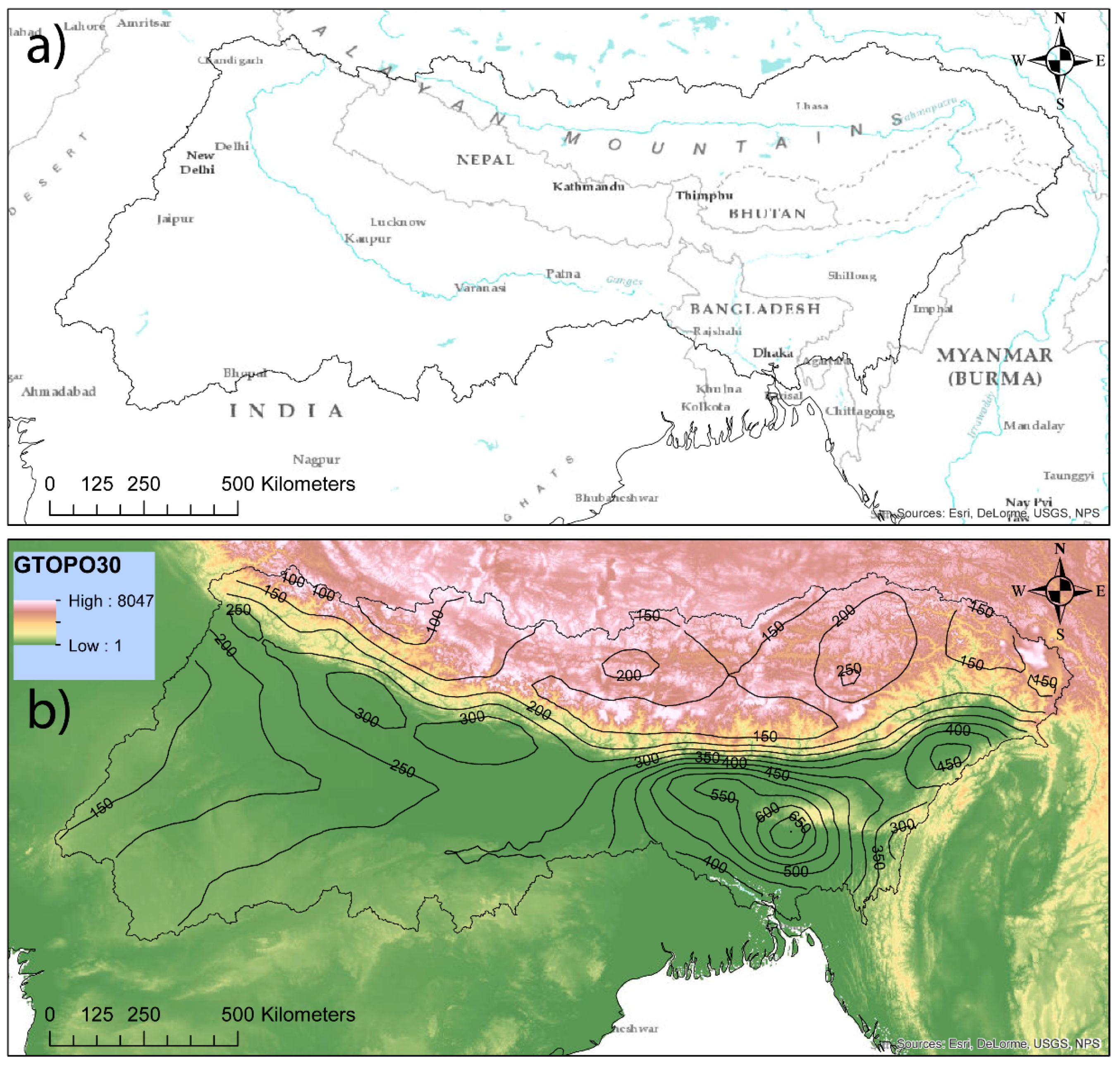
The Ganges–Brahmaputra–Meghna (GBM) river basin is approximately 1.72 million km2 (roughly the size of Iran), intersects five nations: India, China, Nepal, Bangladesh and Bhutan; and contains 630 million people [8] (Figure 1a). It drains the combined Ganges, Brahmaputra and Meghna rivers, where the vast majority of discharge eventually makes its way to the main trunk of the Lower Meghna river/estuary in Bangladesh and into the Bay of Bengal. With a discharge of up to 138,700 m3/s of water during flood periods, it is the largest in the world through a single outlet [8,9]. Precipitation which feeds this immense and powerful river system primarily falls in the monsoon season, with 77% of the total rainfall received in June, July, August and September (JJAS). Therefore, the strength of the monsoon is an important predictor for discharge dynamics in the delta environment, including flooding, which has received much attention in the literature [10]. Riverbank erosion at the GBM outlet is another consequence of high flow rates, but, unlike flooding, land resources are permanently lost, leading to forced societal disruption and reorganization [11]. A recent modeling study of future changes in the hydrology of the GBM suggests that the flooding and erosion hazards will worsen by the end of the 21st century [12]. Five Coupled Model Intercomparison Project Phase 5 members project an increase in runoff by 16% in the Brahmaputra, 33% in the Ganges and 40% in the Meghna river basins by the 2075–2099 time period [12].
Isohyets on Figure 1b indicate the JJAS average rainfall for the period 1983 to 2015. On average over 650 mm mo−1 of rainfall occurs in northern Bangladesh, with a secondary maximum of 450 mm mo−1 over for eastern India. There is a strong precipitation gradient from south to north, with large values (300 mm mo−1) in the foothills of the Himalayas and lower values (200 mm mo–1) on the Tibetan Plateau. Minimum values (100–150 mm mo−1) can be found the northern and western boundaries of the basin.
3. Materials and Methods
Satellite-based estimates of precipitation are useful for examining transnational water issues and hazards in developing countries [13] as they are consistent and complete in time and space. Here we selected the Precipitation Estimation from Remotely Sensed Information using Artificial Neural Networks-Climate Data Record (PERSIANN-CDR), which has some advantages over other products [14], but was not utilized in the GBM studies mentioned in the Introduction [4,5,6,7]. However, PERSIANN-CDR has been found to be useful in hydroclimate studies in India and the Tibetan Plateau [15,16]. PERSIANN-CDR has a high spatial resolution at a 0.25° latitude/longitude grid spacing, which allows for a sub-basin scale analysis and a long data record, extending from 1983 to 2015, which can resolve interannual to interdecadal climate variability. Finally, the PERSIANN-CDR precipitation values are bias corrected to the Global Precipitation Climatology Project (GPCP) version 2.3 estimates, which include gauge information [17], thus maintaining consistency at the monthly scale. GPCP v2.3 (Global Precipitation Climatology Project Version 2.3) was therefore used to examine precipitation anomalies in a global context.
PERSIANN-CDR precipitation was averaged over the monsoon season June-July-August-September (JJAS) and extracted by the GBM boundary using the HydroBASIN GIS layer from the World Wildlife Fund (Gland, Switzerland) [18]. GBM precipitation patterns were then statistically described through Principal Component (PC) analysis in ArcGIS for the 2309 selected cells (see Figure 2). This statistical tool is used to reduce redundancy in multi-dimensional data. Thirty-three functions (eigenvectors) are constructed, which are orthogonal and uncorrelated, containing a covariance matrix of 2309 cells. The first eigenvector explains the greatest variance in a data set and normally most of the variance can be described by the first few eigenvectors (principal components). Each eigenvector has 33 coefficients, representing power as a function of time. The climatological mean was not subtracted prior to deconstructing the data, as is the case in many climate studies [19], as our goal is to understand how climate teleconnections contribute to total water delivery.
The first three PCs were analyzed using the eight sub-basin polygons at Pfafstetter level-04 obtained from the World Wildlife Fund (Gland, Switzerland) [18]. Watersheds were delineated in a consistent manner at different scales and a hierarchical sub-basin breakdown was created following the typological concept of the Pfafstetter coding system. PC eigenvalues were averaged and multiplied by the eigenvector coefficients to return their contribution to the total rainfall per year. Finally, JJAS rainfall was also averaged over the level-04 sub-basins. These sub-basin time series were then correlated with time series of JJAS climate indices, namely Nino 3.4, defined as SST anomalies averaged over the box: 5° N, 5° S; 170°–120° W and the Tropical Southern Atlantic Index (TSA), defined as SST anomalies averaged over the box: 10° E, 30° W; 0°–20° S [20]. Two-meter air temperature, 850 hPa heights, 850 hPa zonal wind stress and 200 hPa heights were retrieved for the same JJAS season and 1983–2015 time period from the ECMWF ERA-Interm reanalysis [21]. These fields and GPCP v2.3 were related to the PC eigenvector coefficients through linear correlation and regression analyses.
4. Results
4.1. GBM Precipitation Analysis
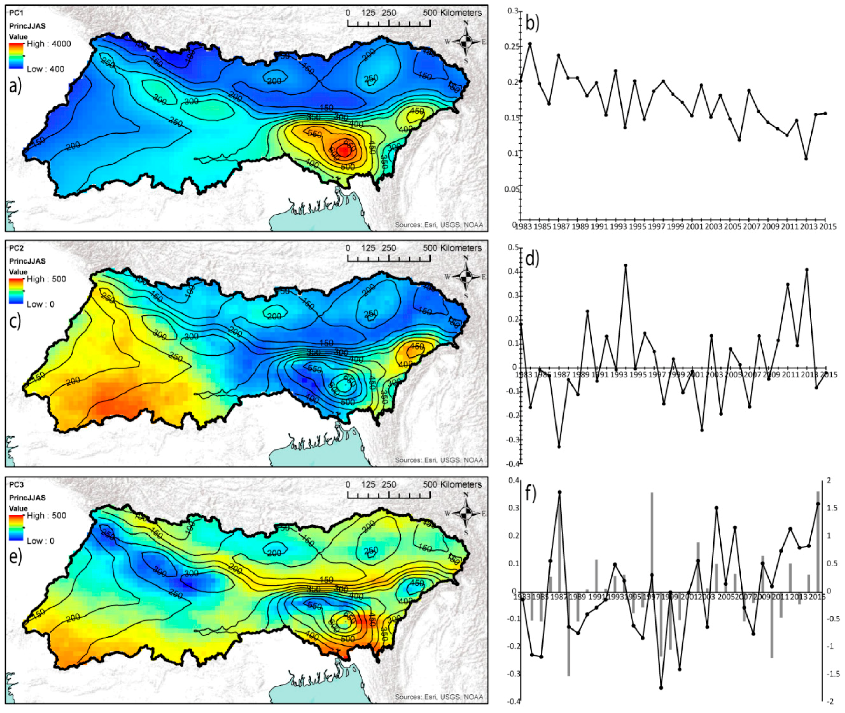
The first PC (PC1) explains 88.7% of the variance of precipitation in the GBM (Figure 2a) and represents the background climatology (see contours). The maximum is located in northeast Bangladesh with two axes of higher values to the northeast and northwest along the Himalayan ridge and a secondary maximum over far-eastern India. The eigenvector coefficient is positive every year, meaning this pattern is a consistently strong feature, with little interannual variability and a downward trend (Figure 2b), which is consistent with other studies that suggest a downward trend in monsoonal rainfall over this time period [5,7]. The second PC (PC2) explains 2.9% of the variance. The values are much lower than PC1, with two maxima (Figure 2c). The first coincides with the maximum in PC1 over far-eastern India and the second is over central India. The eigenvector coefficients have a mean near zero and large interannual variability. There is also an apparent decadal-scale cycle, with the 1980s and 2000s being mostly negative and the 1990s and 2010s mostly positive (Figure 2d). The third PC (PC3) explains 1.5% of the variance. The values are comparable with PC2, but the spatial pattern includes smaller-scale variability (Figure 2e). High values can be found at the southern border of the GBM. A second maximum occurs over the climatological precipitation gradient (see contours). To the north and south are minima, resulting in an overall zonally banded structure. The PC3 coefficients have strong interannual variability (Figure 2f).
4.2. Global Climate Analysis
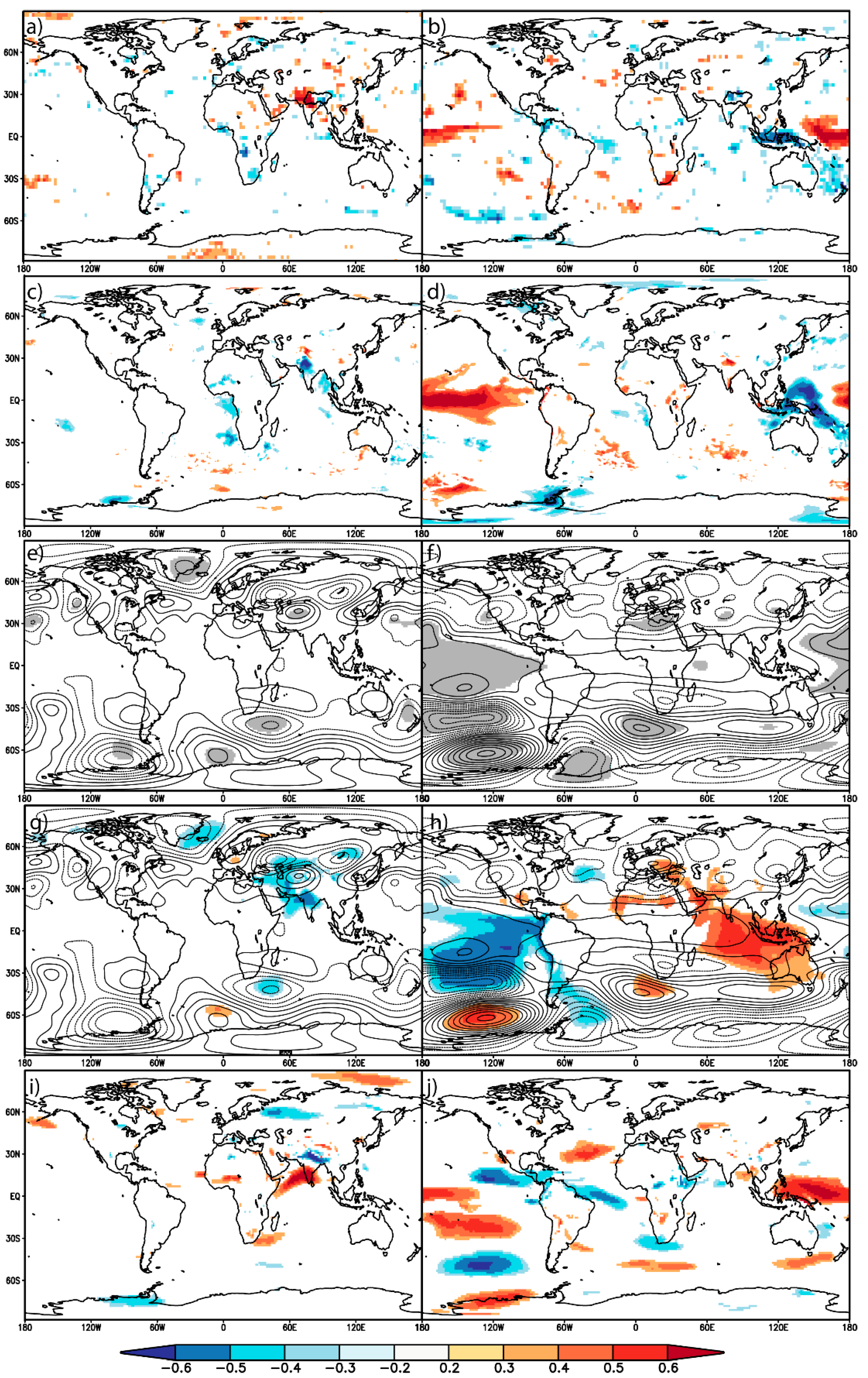
Hereon we focus on PC2 and PC3, which contain the largest year-to-year variability. After detrending the eigenvector coefficients, the standard deviations were computed as 0.03, 0.17 and 0.16 for PC1, PC2 and PC3 respectively. The coefficients of PC2 and PC3 were then field correlated to JJAS averaged GPCP precipitation to determine if the GBM patterns were part of a larger global rainfall signal. The GPCP analysis confirms that when PC2 is strong rainfall is abundant over northern to central India, with a decline in rainfall over Bangladesh (Figure 3a). GPCP cannot capture the small-scale spatial variability of the PC3 pattern (Figure 2e), but picks up the low rain rates (negative correlations) in the northwest to northern reaches of the GBM (Figure 3b). While there is some extension of the PC-GPCP correlations outside the basin, they appear to be relatively localized. Furthermore, only the PC3 map has areas of organized correlations distant to the GBM (Figure 3c). The negative correlations over Indonesia and positive correlations around 180° are consistent with a Central-Pacific El Niño. This is confirmed, as the PC3 coefficients are significantly positively correlated with Nino 3.4 (r = +0.66, p < 0.01), suggesting that monsoonal precipitation anomalies during El Niño should mirror the pattern in Figure 3e (also see the Nino 3.4 time series in Figure 2f). Further, the detrended time series of precipitation averaged over the entire GBM was found to be significantly negatively correlated with Nino 3.4 (r = −0.46, p < 0.01). Previous studies have shown that ENSO is the leading mode of variability in the South Asian summer monsoon, especially over India, where a warm central to eastern Pacific leads to dry conditions [22]. However, it should be noted that the large-scale response of the monsoon to ENSO depends on whether ENSO is developing or decaying [23,24] and the ENSO-monsoon relationship varies interdecadally [25,26].
With regards to surface temperature, PC2 is related to a cooling over the Gulf of Guinea and Bay of Bengal (Figure 3d,e). The relationship between heating in the South Atlantic and the contemporaneous decline in rainfall in India has also been noted previously [27] and has been explained by a Gill-Matsuno-type quadrupole. TSA was correlated to the detrended time series of the eigenvector coefficients of PC2 and GBM average rainfall. With an r of +0.45 (p < 0.01), GBM precipitation is equally related to SST anomalies in the South Atlantic as in the Pacific (i.e., ENSO) and PC2 and TSA are negatively correlated (r = −0.37; p < 0.05), consistent with Figure 3c. Examining Figure 3d, the PC3-ENSO relationship is substantiated, with correlations consistent with a warm central Pacific and cool western Pacific.
PC2 shows a succession of significant upper-tropospheric pressure anomalies emanating from the North Atlantic to the GBM region (Figure 3e). This was described previously [2] and related to warm surface temperatures over Iran. However, in our study the upper-tropospheric wave train is shifted eastward compared to the results from [2] and the positive correlations between surface temperature and PC2 are also east of Iran (Figure 3c). The addition of significant 850 hPa correlations, shows lower heights over northwestern India (Figure 3g), which is consistent with a warm troposphere, convective instability and rainfall in the western GBM (Figure 3a). A similar result was also found by [28] when they regressed 850 hPa heights with the regional maximum covariance analysis of tropical Atlantic SST and South Asia precipitation [28]. Interestingly, significant PC2-850 hPa correlation values extend from India into the surrounding areas over the Arabian Sea, Iran and an eastward extension into the western portion of the GBM (Figure 3g). PC3 correlations with 200 hPa heights are consistent with a warm tropical troposphere (Figure 3f) and 850 hPa height correlations are negative over much of the tropical Pacific Ocean, but positive over the Indian Ocean suggesting higher pressure and an altered monsoon circulation (Figure 3h). Positive correlations also extend from the Indian Ocean into Europe through the Arabian Peninsula.
Finally, the PC2 850 hPa zonal wind stress correlations (Figure 3i) are consistent with the 850 hPa height correlations over India. To the north (south) of the negative PC2-850 hPa correlation in the same area are found significantly negative (positive) wind stress correlations, indicating cyclonic flow (Figure 3i). The PC3 correlations in the vicinity of the GBM are weaker than PC2, although positive values in the Bay of Bengal and negative values in the Arabian Sea suggest near-surface divergence and advection of moisture away from the GBM (Figure 3j). Consistent with this picture, PC3 is positively correlated with precipitation over the Indochinese Peninsula (Figure 2b). Finally, Figure 3j shows an abundance of positive values in the tropical Pacific Ocean consistent with a weakened Walker Circulation.
4.3. Sub-Basin Scale Analysis
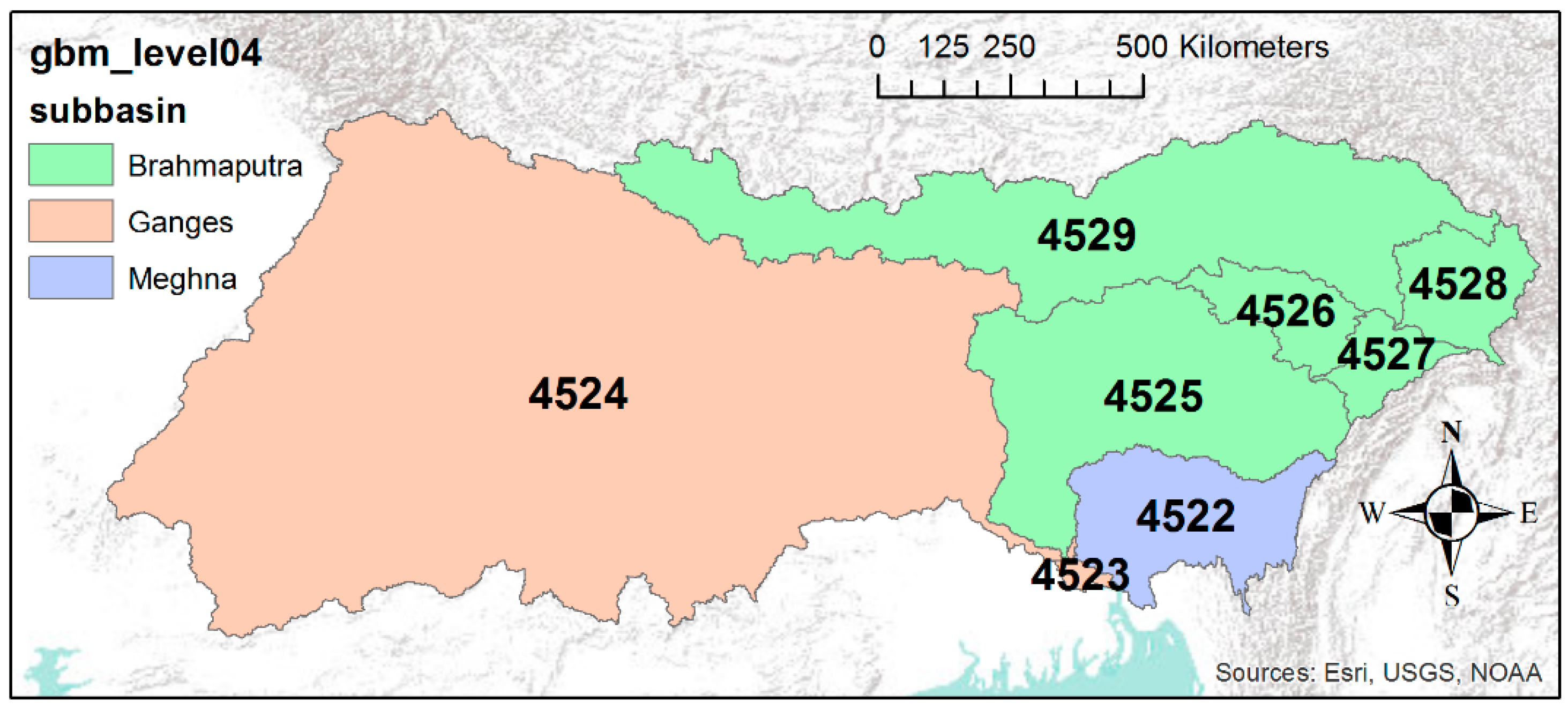
Figure 4 shows the Pfafstetter level-04 sub-basin boundaries of the GBM obtained from the World Wildlife Fund (Gland, Switzerland): two containing the Ganges, five the Brahmaputra and one the Meghna. On average it rains the most in the Meghna (Table 1 and contours in Figure 1), but the precipitation contributes only 10% to the total water volume of the river system. The average rainfall in the western Ganges (4524) is slightly lower than the overall GBM mean of 250.4 mm mo−1, but because of its vast size (~257,000 km2) it contributes 56% of the total water (Table 1). The southwest Brahmaputra (4525) and northern Brahmaputra (4529) are significant in size and contribute slightly more than the Meghna to the total (Table 1). The sub-basin average of PC2 and PC3 are found in the third and fourth columns of Table 1. Multiplying these averages by their eigenvector coefficients yields the precipitation contributed by these climate modes for each monsoon season. In order to determine the greatest impact these climate patterns had on sub-basin scale rainfall from 1983 to 2015, the maximum eigenvector coefficients were selected for evaluation (Table 1). For PC2 it was 0.43 and occurred in 1994 and for PC3 it was 0.36 and occurred in 1987 (Figure 2b,c). The fifth and sixth columns of Table 1 give the resulting average rainfall values for these years. PC2’s largest rainfall amount was 139.4 mm mo−1 in southeastern Brahmaputra (4527) and PC1’s largest was 158.6 mm mo−1 in eastern Ganges (4523). However, this does not consider the contribution to the total rainfall for the selected years. Dividing by the average rainfall in each sub-basin for the two selected years yields the results in columns seven and eight in Table 1. In 1994, PC2 contributed a maximum of 44% of the total rainfall in western Ganges (4524) and in 1987 PC3 contributed a maximum of 51% of the total rainfall in northern Brahmaputra (4529).
It was already established that PC3 is significantly related to ENSO and the GBM as a whole is anomalously dry during El Niño. Furthermore, PC2 is significantly related to tropical South Atlantic SST and the GBM is anomalously wet when the temperatures are warm. Table 1 refines these relationships further, with correlations between average precipitation at the sub-basin level (the eight-time series were also detrended) and the two climate indices. Interestingly, only precipitation over the western Ganges (4524) and northern Brahmaputra (4529) seem to contribute to the overall negative ENSO relationship. In fact, these correlations (−0.51 and −0.50) are larger than for the GBM as a whole (−0.47). This agrees with a recent study where June to October precipitation anomalies at the pixel scale in the GBM were composited by El Niño and La Niña years [6]. They found that dry conditions dominated the western and southeastern portions of the Ganges basin in El Niño years, while wet conditions were found in the eastern parts of the Ganges basin, extending into the far western reaches of the Brahmaputra basin during La Niña years. Reexamining the map of PC3 (Figure 2c), it is clear that when the eigenvector coefficient is strongly positive (consistent with El Niño conditions, such as in 1987), precipitation is anomalously low in these same regions. All sub-basins, except the southeast Brahmaputra (4527), have a positive relationship with tropical South Atlantic SST and four are statistically significant. The strongest relationships are located in the center of the GBM, including northern Brahmaputra (4529), which has a correlation of +0.60. In fact, the Atlantic has a greater association with rainfall than the central Pacific in all sub-basins except the western Ganges (4524). Another study also found a similar pattern of South Asian monsoon precipitation related to tropical Atlantic SST variability, where positive correlations extended from Bangladesh northward through southern China [28].
5. Discussion
Principal components were used to distinguish the first three climate modes of precipitation within the GBM. The primary mode (PC1), is focused over the Meghna river basin every year, but with an overall downward trend. The second and third climate modes (PC2 and PC3) explain more interannual to interdecadal variability, especially in the northern and western portions of the basin. A likely contributor to the PC2 pattern is tropical South Atlantic temperatures [27], but PC2 might also have a mid-latitude origin via a Rossby wave train extending from the North Atlantic to South Asia [2]. However, both set-ups are consistent with lower 850 hPa heights extending from India into the Arabian Sea and cyclonic flow. This leads to westerly winds sweeping across the Arabian Sea, bringing abundant moisture into the Indian peninsula and enhancing rainfall. The opposite scenario appears to be the case for years when Bangladesh receives more rainfall than normal. The third climate mode (PC3) was related to ENSO, which instigates high pressure anomalies over the Indian Ocean. This high pressure extends northwestward, but Figure 3h also suggests a ridge building eastward along the foothills of the Himalayas, which may lead to the zonal band of lower rainfall in Figure 2e and Figure 3b. However, further investigation with finer-scale climate data is warranted.
Although PC1 mimics the overall GBM climatology and contributes the bulk of the precipitation, PC2 and PC3 can contribute up to 50% of the rainfall within the Pfafstetter level-04 sub-basins during years when these modes are strong. ENSO and tropical South Atlantic temperatures also showed some potential for hydroclimatological predictability at the sub-basin scale. ENSO is significantly correlated with precipitation averaged over the two largest sub-basins, covering 76.5% of the area and contributing 67.3% of the water. Tropical South Atlantic temperature is significantly correlated with precipitation averaged over the central sub-basins of the GBM, covering 30.3% of the area and contributing 29.7% of the water. Interestingly, northern Brahmaputra rainfall seems to be related to both ENSO and tropical South Atlantic temperature and holds the highest promise for climate prediction.
6. Conclusions
Improved understandings of annual changes in GBM precipitation is important for managing water resources and preparing for hydrologic hazards. Most of the GBM rainfall occurs in the monsoon months of June, July, August and September, but there is high spatial and interannual variability. Reducing this complexity to a few climate modes of precipitation has helped to identify the sources of atmospheric moisture and uplift that dictate the locations of rainfall in the basin and the precursor climate forcings that serve to alter the large-scale atmospheric circulation. Finally, this is the first study to investigate hydroclimate teleconnections at the sub-basin scale in the GBM. Going from the basin as a whole to regional hydrologic units actually serves to strengthen the precipitation relationships with ENSO and the South Atlantic, thus encouraging downscaled hydroclimate predictions in the GBM.
Author Contributions
Conceptualization, S.C.; Methodology, S.C.; Software, S.C.; Formal Analysis, S.C., M.P.; Writing-Original Draft Preparation, S.C.; Writing-Review & Editing, S.C., T.C., M.R., M.G.M., M.R.I.; Visualization, S.C., M.P.; Project Administration, T.C.; Funding Acquisition, T.C., S.C., M.R., B.P., M.G.M., M.R.I.
Funding
This research was funded by the U.S. National Science Foundation grant number 1660447. The APC was funded by East Carolina University.
Acknowledgments
Conflicts of Interest
The authors declare no conflict of interest. The funders had no role in the design of the study; in the collection, analyses, or interpretation of data; in the writing of the manuscript and in the decision to publish the results.
References
- McGregor, G. Hydroclimatology, modes of climatic variability and stream flow, lake and groundwater level variability. Prog. Phys. Geogr. 2017, 41, 496–512. [Google Scholar] [CrossRef] [Green Version]
- Yadav, R.K. On the relationship between Iran surface temperature and northwest India summer monsoon rainfall. Int. J. Climatol. 2016, 36, 4425–4438. [Google Scholar] [CrossRef]
- Choi, J.-W.; Cha, Y.; Lu, R. Interdecadal variation of summer monsoon over the southern part of Asia in mid-1990s. Int. J. Climatol. 2017, 37, 1138–1146. [Google Scholar] [CrossRef]
- Ashok, K.; Saji, N.H. On the impacts of ENSO and Indian Ocean dipole events on sub-regional Indian summer monsoon rainfall. Nat. Hazards 2007, 42, 273–285. [Google Scholar] [CrossRef]
- Khandu; Awange, J.L.; Kuhn, M.; Anyah, R.; Forootan, E. Changes and variability of precipitation and temperature in the Ganges-Brahmaputra-Meghna river basin based on global high-resolution reanalyses. Int. J. Climatol. 2017, 37, 2141–2159. [Google Scholar]
- Pervez, M.S.; Henebry, G.M. Spatial and seasonal responses of precipitation in the Ganges and Brahmaputra river basins to ENSO and Indian Ocean dipole modes: implications for flooding and drought. Nat. Hazards Earth Syst. Sci. 2015, 15, 147–162. [Google Scholar] [CrossRef] [Green Version]
- Khandu; Awange, J.L.; Anyah, R.; Kuhn, M.; Fukuda, Y. Assessing regional climate simulations of the last 30 years (1982–2012) over Ganges-Brahmaputra-Meghna River Basin. Clim. Dyn. 2017, 49, 2329–2350. [Google Scholar]
- Frenken, K. Irrigation in Southern and Eastern Asia in Figures; Food and Agriculture Organization (FAO): Rome, Italy, 2012; Available online: www.fao.org/nr/water/aquastat/basins/gbm/index.stm (accessed on 1 November 2017).
- Chowdhury, M.R.; Ward, N. Hydro-meteorological variability in the greater Ganges-Brahmaputra-Meghna basins. Int. J. Climatol. 2004, 24, 1495–1508. [Google Scholar] [CrossRef] [Green Version]
- Islam, A.S.; Haque, A.; Bala, S.K. Hydrologic characteristics of floods in Ganges-Brahmaputra-Meghna (GBM) delta. Nat. Hazards 2010, 54, 797–811. [Google Scholar] [CrossRef]
- Mutton, D.; Haque, C.E. Human vulnerability, dislocation and resettlement: Adaptation processes of river-bank erosion-induced displacees in Bangladesh. Disasters 2004, 28, 41–62. [Google Scholar] [CrossRef]
- Masmood, M.; Yeh, P.J.-F.; Hanasaki, N.; Takeuchi, K. Model study of the impacts of future climate change on the hydrology of Ganges-Brahmaputra-Meghna basin. Hydrol. Earth Syst. Sci. 2015, 19, 747–770. [Google Scholar] [CrossRef]
- Hossain, F.; Katiyar, N.; Hong, Y.; Wolf, A. The emerging role of satellite rainfall data in improving the hydro-political situation of flood monitoring in the under-developed regions of the world. Nat. Hazards 2007, 43, 199–210. [Google Scholar] [CrossRef]
- Ashouri, H.; Hsu, K.L.; Sorooshian, S.; Braithwaite, D.K.; Knapp, K.R.; Cecil, L.D.; Nelson, B.R.; Prat, O.P. PERSIANN-CDR: Daily precipitation climate data record from multisatellite observations for hydrological and climate studies. Bull. Am. Meteorol. Soc. 2015, 96, 69–83. [Google Scholar] [CrossRef]
- Liu, X.; Yang, T.; Hsu, K.; Liu, C.; Sorooshian, S. Evaluating the streamflow simulation capability of PERSIANN-CDR daily rainfall products in two river basins on the Tibetan Plateau. Hydrol. Earth Syst. Sci. 2017, 21, 169–181. [Google Scholar] [CrossRef] [Green Version]
- Mondal, A.; Lakshmi, V.; Hashemi, H. Intercomparison of trend analysis of multisatellite monthly precipitation products and gauge measurements for river basins of India. J. Hydrol. 2018, 565, 779–790. [Google Scholar] [CrossRef]
- Adler, R.F.; Huffman, G.J.; Chang, A.; Ferraro, R.; Xie, P.; Janowiak, J.; Rudolf, B.; Schneider, U.; Curtis, S.; Bolvin, D.; Gruber, A.; Susskind, J.; Nelkin, E.; et al. The version 2 Global Precipitation Climatology Project (GPCP) monthly precipitation analysis (1979–present). J. Hydromet. 2003, 4, 1147–1167. [Google Scholar] [CrossRef]
- Lehner, B.; Grill, G. Global river hydrography and network routing: Baseline data and new approaches to study the world’s largest river systems. Hydrol. Process. 2013, 27, 2171–2186. [Google Scholar] [CrossRef]
- Dai, A.; Wigley, T.M.L. Global patterns of ENSO induced precipitation. Geophys. Res. Lett. 2000, 27, 1283–1286. [Google Scholar] [CrossRef]
- Enfield, D.B.; Mestas-Nuñez, A.M.; Mayer, D.A.; Cid-Serrano, L. How ubiquitous is the dipole relationship in tropical Atlantic sea surface temperatures? J. Geophys Res. Oceans 1999, 104, 7841–7848. [Google Scholar] [CrossRef] [Green Version]
- Dee, D.P.; Uppala, S.M.; Simmons, A.J.; Berrisford, P.; Poli, P.; Kobayashi, S.; Andrae, U.; Balmaseda, M.A.; Balsamo, G.; Bauer, P. The ERA-Interim reanalysis: Configuration and performance of the data assimilation system. Q. J. R. Met. Soc. 2011, 137, 553–597. [Google Scholar] [CrossRef]
- Mishra, V.; Smoliak, B.V.; Lettenmaier, D.P.; Wallace, J.M. A prominent pattern of year-to-year variability in Indian summer monsoon rainfall. Proc. Natl. Acad. Sci. USA 2012, 109, 7213–7217. [Google Scholar] [CrossRef] [PubMed]
- Wang, B.; Yang, J.; Zhou, T.; Wang, B. Interdecadal changes in the major modes of Asian-Australian monsoon variability: Strengthening relationships with ENSO since the late 1970s. J. Clim. 2008, 21, 1771–1789. [Google Scholar] [CrossRef]
- Xie, S.-P.; Hu, K.; Hafner, J.; Tokinaga, H.; Du, Y.; Huang, G.; Sampe, T. Indian Ocean capacitor effect on Indo-western Pacific climate during the summer following El Niño. J. Clim. 2009, 22, 730–747. [Google Scholar] [CrossRef]
- Krishna Kumar, K.; Rajagopalan, B.; Cane, M.A. On the weakening relationship between the Indian monsoon and ENSO. Science 1999, 284, 2156–2159. [Google Scholar] [CrossRef]
- Kucharski, F.; Bracco, A.; Yoo, J.H.; Molteni, F. Low-frequency variability of the Indian monsoon-ENSO climate relationship and the tropical Atlantic: The “weakening” of the 1980s and 1990s. J. Clim. 2007, 20, 4255–4266. [Google Scholar] [CrossRef]
- Kucharski, F.; Bracco, A.; Yoo, J.H.; Tompkins, A.M.; Feudale, L.; Ruti, P.; Dell’Aquila, A. A Gill-Matsuno-type mechanism explains the tropical Atlantic influence on African and Indian monsoon rainfall. Q. J. R. Met. Soc. 2009, 135, 569–579. [Google Scholar] [CrossRef] [Green Version]
- Syed, F.S.; Kucharski, F. Statistically related coupled modes of South Asian summer monsoon interannual variability in the tropics. Atmos. Sci. Lett. 2016, 17, 183–189. [Google Scholar] [CrossRef]
- Koninklijk Nederlands Meteorologisch Instituut Climate Explorer. Available online: https://climexp.knmi.nl (accessed on 1 November 2017).
Figure 1.
Ganges–Brahmaputra–Meghna (GBM) study area with (a) major rivers and political boundaries and (b) elevation in meters (colors) and June-July-August-September (JJAS) 1983 to 2015 precipitation climatology in mm mo−1 (contours).
Figure 1.
Ganges–Brahmaputra–Meghna (GBM) study area with (a) major rivers and political boundaries and (b) elevation in meters (colors) and June-July-August-September (JJAS) 1983 to 2015 precipitation climatology in mm mo−1 (contours).

Figure 2.
June-July-August-September (JJAS) precipitation patterns in the GBM from 1983 to 2015 as revealed by principal component (PC) analysis. Contours are climatological precipitation as in Figure 1. (a) the first eigenvector or PC1; (b) PC1’s coefficients for each year; (c) the second eigenvector or PC2; (d) PC2’s coefficients for each year; (e) the third eigenvector or PC3; (f) PC3’s eigenvector coefficients for each year. Bars in (f) show the JJAS averaged Nino 3.4 index.

Figure 3.
Correlations significant at the 95th percentile between eigenvector coefficients (see Figure 1) and June-July-August-September averaged global atmospheric fields from 1983 to 2015. See color bar for scale. Contours in (e–h) are regressions of the coefficients with 200 hPa heights. The solid (dashed) lines represent positive (negative) values and shading is significance at the 95th percentile. Increments are 200 m. The GBM boundary is outlined in (a) and (b). (a) precipitation and PC2; (b) same as (a), but PC3; (c) 2-meter air temperature and PC2; (d) same as (c), but PC3; (e) 200 hPa heights and PC2; (f) same as (e) but PC3; (g) 850 hPa heights and PC2; (h) same as (g) but PC3; (i) 850 hPa zonal wind stress and PC2; (j) same as (i) but PC3.

Figure 4.
Boundaries of the Pfafstetter level-04 hydrologic units for the GBM. Colors denote Brahmaputra, Ganges, or Meghna basins. Number is the Pfafstetter identification code.
Figure 4.
Boundaries of the Pfafstetter level-04 hydrologic units for the GBM. Colors denote Brahmaputra, Ganges, or Meghna basins. Number is the Pfafstetter identification code.


Table 1.
Statistics for the eight Pfafstetter level-04 hydrologic units (see Figure 3). 1983–2015 climatological rainfall and percentage of total water delivery, PC2 and PC3 averages, average PC2 and PC3 rainfall for 1994 and 1987 respectively, percent of the total rainfall contributed by PC2 and PC3 for 1994 and 1987 respectively and correlation coefficient between June-July-August-September (JJAS) average precipitation and JJAS Nino 3.4 and TSA from 1983 to 2015.
| Sub-Basin | Clim Rain mm mo−1 | Average PC2 | Average PC3 | PC2 1994 mm mo−1 | PC3 1987 mm mo−1 | % of Total PC2 1994 | % of Total PC3 1987 | r Rain vs. Nino 3.4 | r Rain vs. TSA |
|---|---|---|---|---|---|---|---|---|---|
| Meghna (4522) | 480.8 (10.1%) | 181 | 362 | 77.7 | 131.2 | 19 | 22 | +0.03 | +0.33 |
| E Ganges (4523) | 383.9 (0.5%) | 113 | 438 | 48.5 | 158.6 | 18 | 37 | +0.20 | +0.35 1 |
| W Ganges (4524) | 234.0 (56.0%) | 261 | 241 | 111.9 | 87.3 | 44 | 38 | −0.51 2 | +0.29 |
| SW Brahm. (4525) | 338.3 (15.9%) | 142 | 272 | 60.7 | 98.6 | 21 | 24 | −0.09 | +0.35 1 |
| C Brahm. (4526) | 240.3 (2.0%) | 128 | 277 | 54.8 | 100.4 | 28 | 33 | −0.16 | +0.50 2 |
| SE Brahm. (4527) | 406.2 (2.5%) | 325 | 240 | 139.4 | 87.0 | 34 | 18 | +0.04 | −0.07 |
| E Brahm. (4528) | 187.6 (1.9%) | 103 | 271 | 44.1 | 98.0 | 30 | 39 | +0.16 | +0.22 |
| N Brahm. (4529) | 169.3 (11.3%) | 114 | 235 | 48.7 | 85.1 | 36 | 51 | − 0.50 2 | + 0.60 2 |
1 Correlation significant at the 95th percentile (p = 0.05); 2 Correlation significant at the 99th percentile (p = 0.01).
© 2018 by the authors. Licensee MDPI, Basel, Switzerland. This article is an open access article distributed under the terms and conditions of the Creative Commons Attribution (CC BY) license (http://creativecommons.org/licenses/by/4.0/).
Share and Cite
MDPI and ACS Style
Curtis, S.; Crawford, T.; Rahman, M.; Paul, B.; Miah, M.G.; Islam, M.R.; Patel, M. A Hydroclimatological Analysis of Precipitation in the Ganges–Brahmaputra–Meghna River Basin. Water 2018, 10, 1359. https://doi.org/10.3390/w10101359
AMA Style
Curtis S, Crawford T, Rahman M, Paul B, Miah MG, Islam MR, Patel M. A Hydroclimatological Analysis of Precipitation in the Ganges–Brahmaputra–Meghna River Basin. Water. 2018; 10(10):1359. https://doi.org/10.3390/w10101359
Chicago/Turabian StyleCurtis, Scott, Thomas Crawford, Munshi Rahman, Bimal Paul, M. Giashuddin Miah, M. Rafiqul Islam, and Mohin Patel. 2018. "A Hydroclimatological Analysis of Precipitation in the Ganges–Brahmaputra–Meghna River Basin" Water 10, no. 10: 1359. https://doi.org/10.3390/w10101359
Note that from the first issue of 2016, this journal uses article numbers instead of page numbers. See further details here.