
Study of the Characteristics of the Long-Term Persistence of Hourly Wind Speed in Xinjiang Based on Detrended Fluctuation Analysis

Abstract
:1. Introduction
2. Materials and Methods
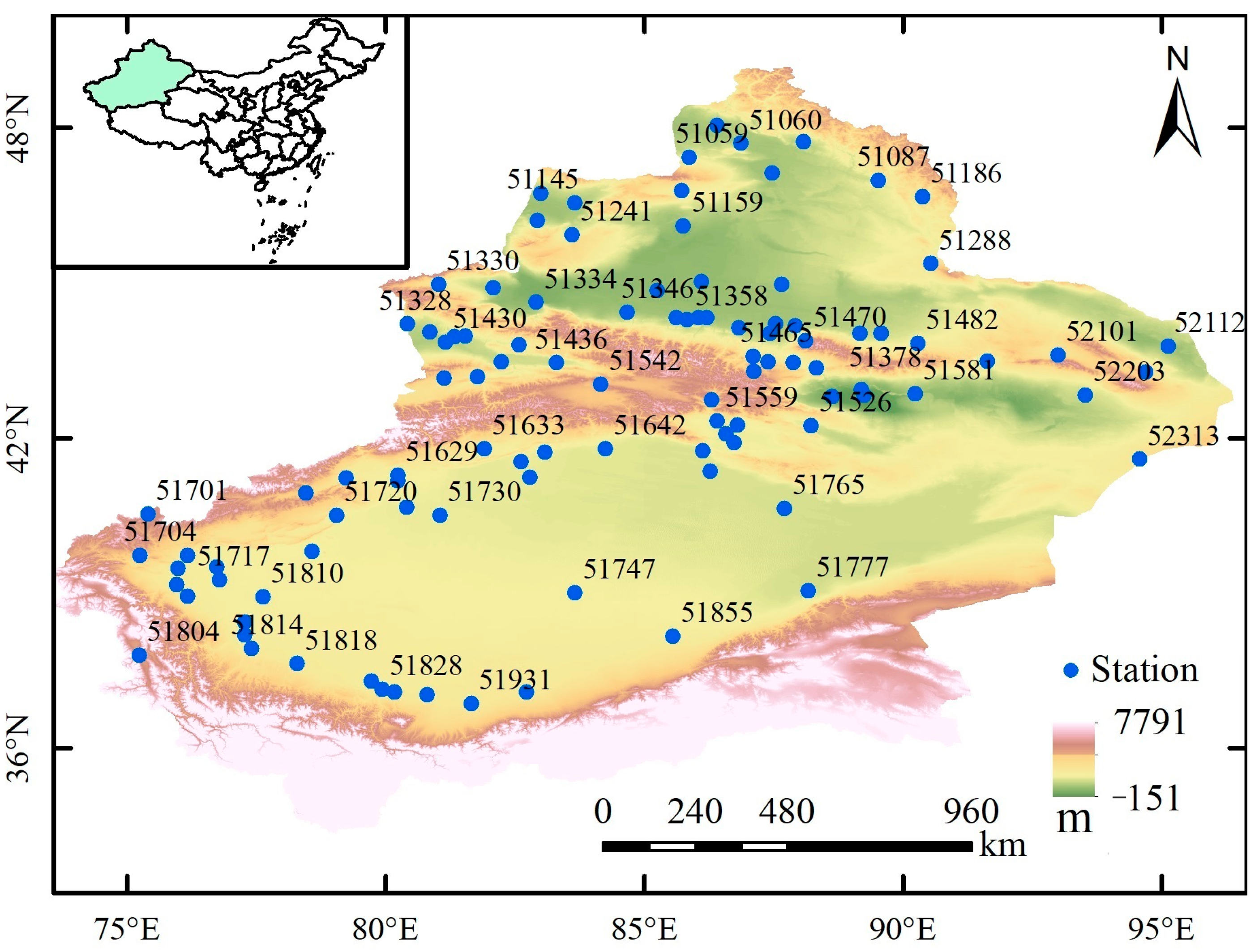
2.1. Study Region and Data Source
2.2. Methodology
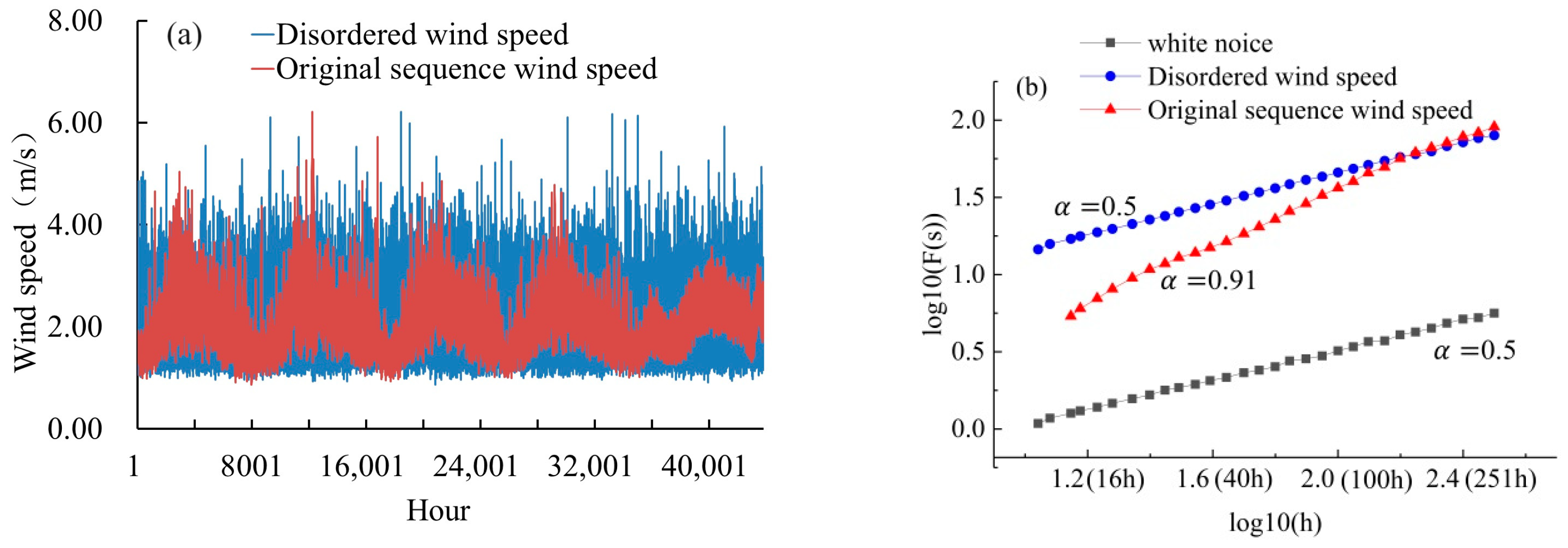
2.2.1. DFA
2.2.2. Discreteness Analysis
3. Results
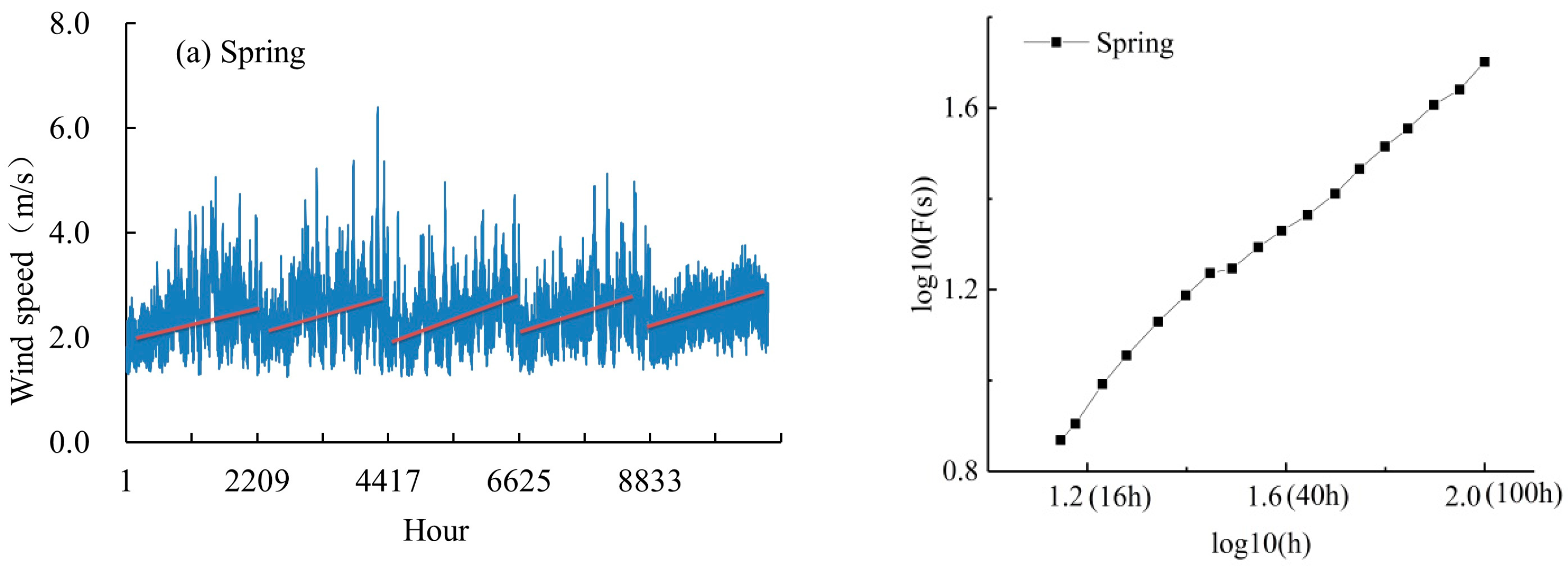
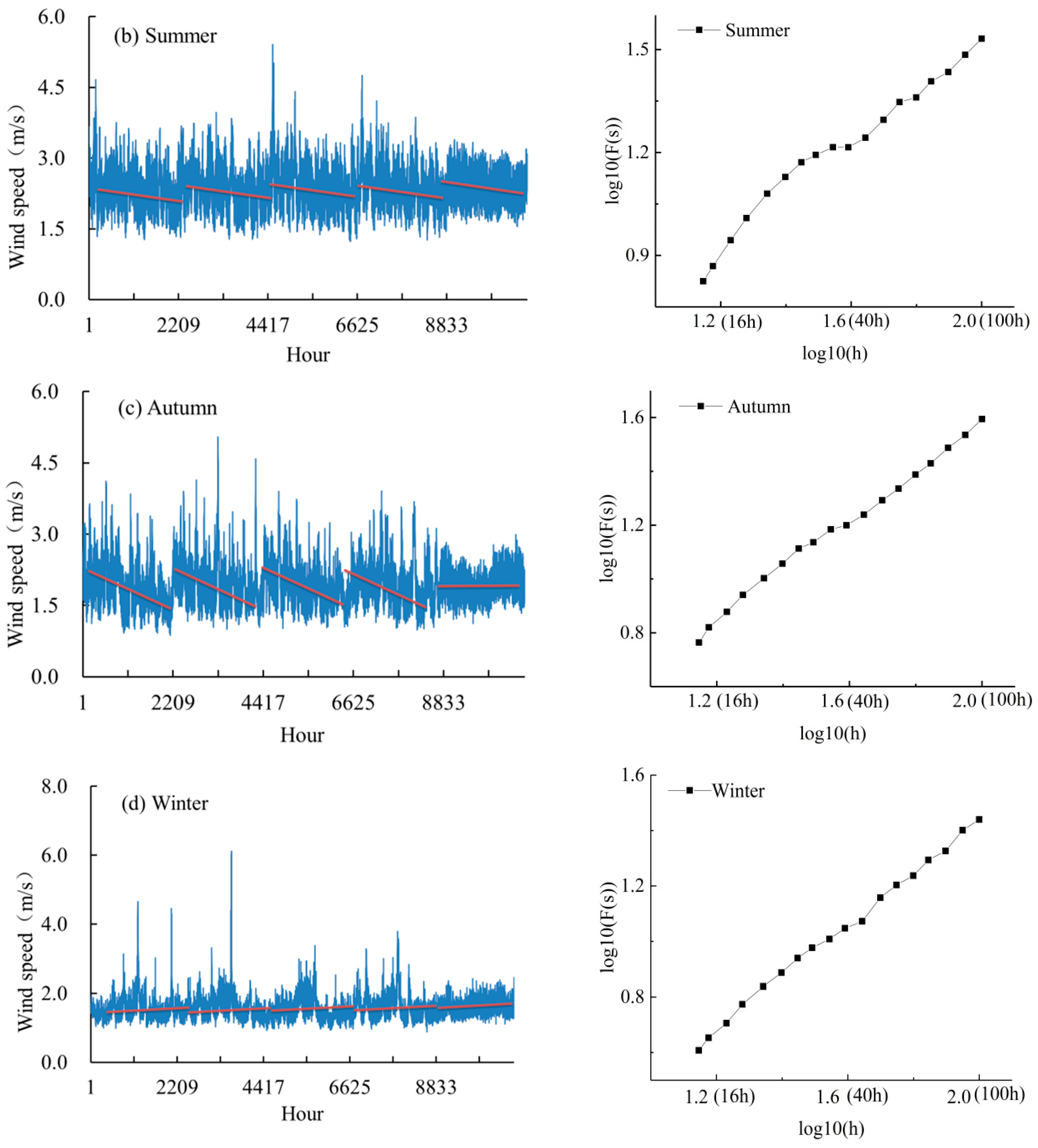
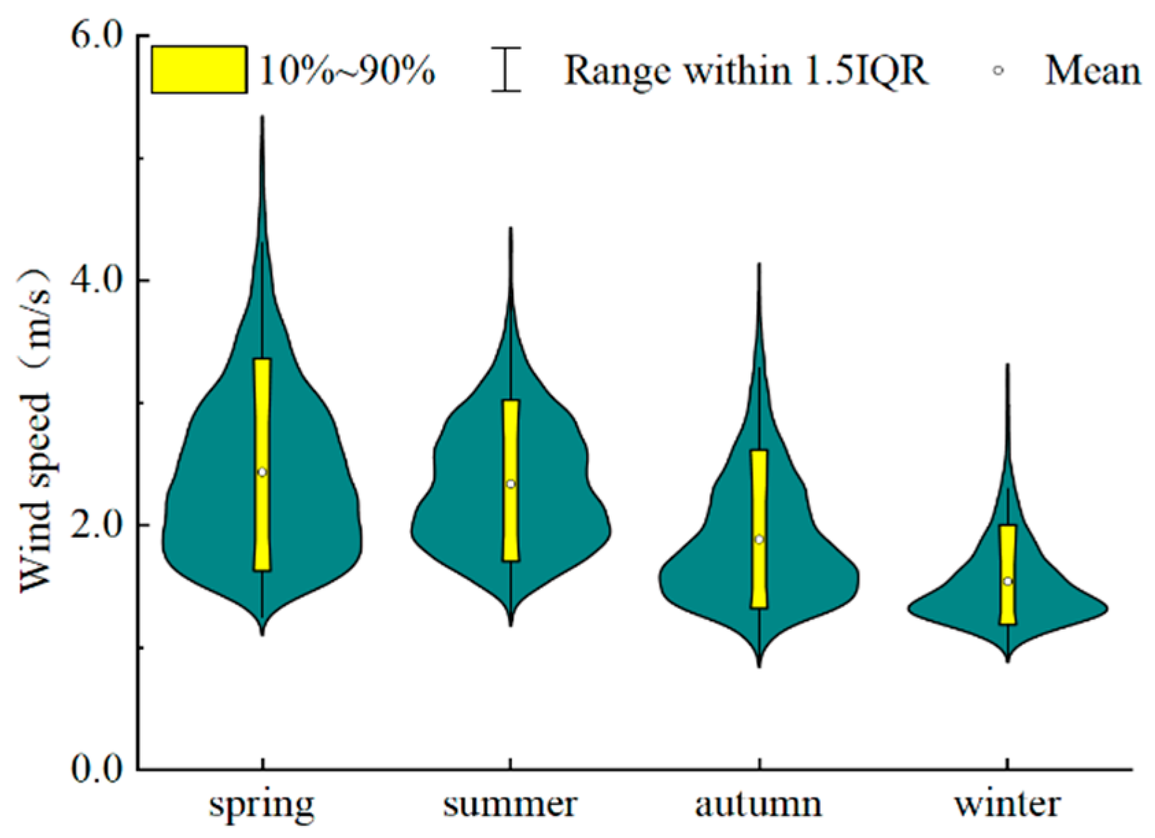
3.1. Seasonal Distribution Characteristics
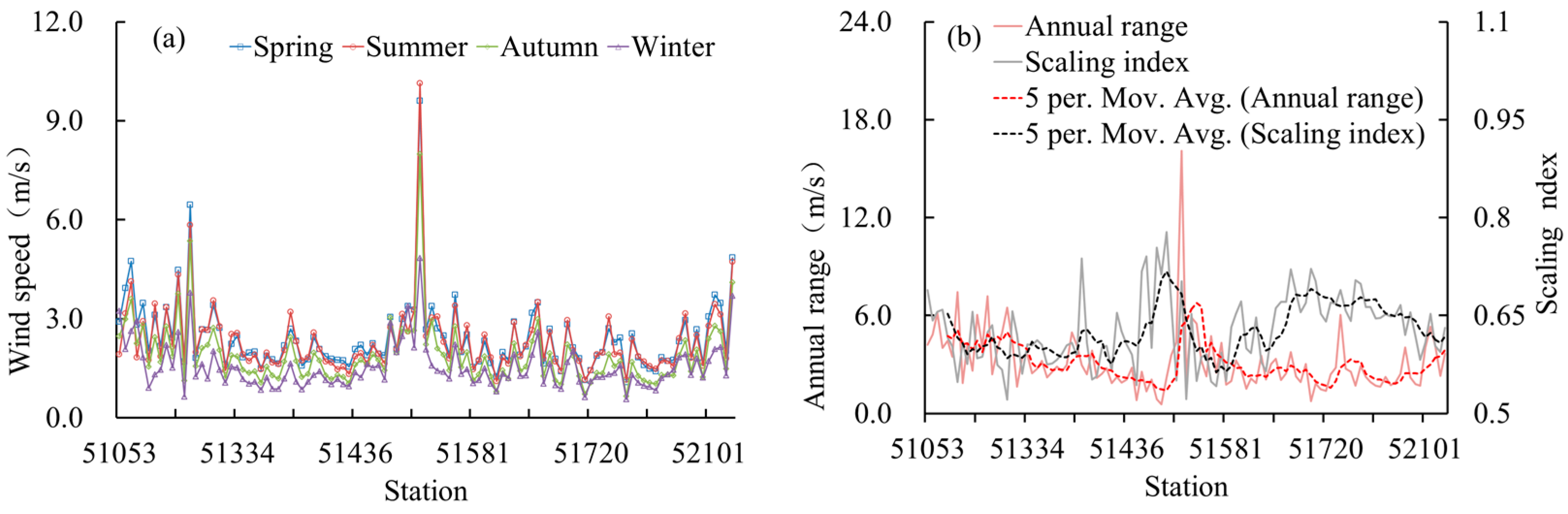
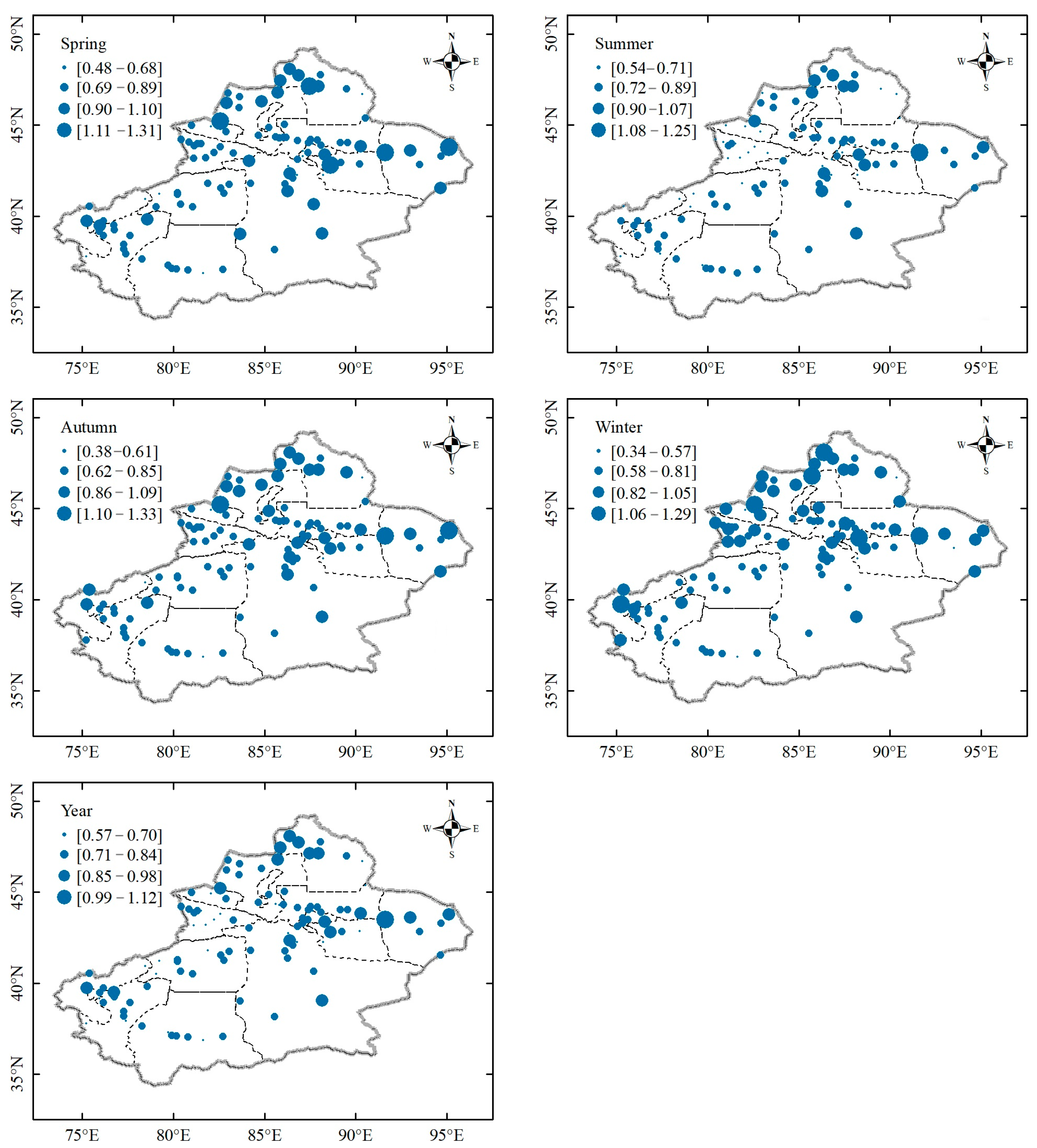
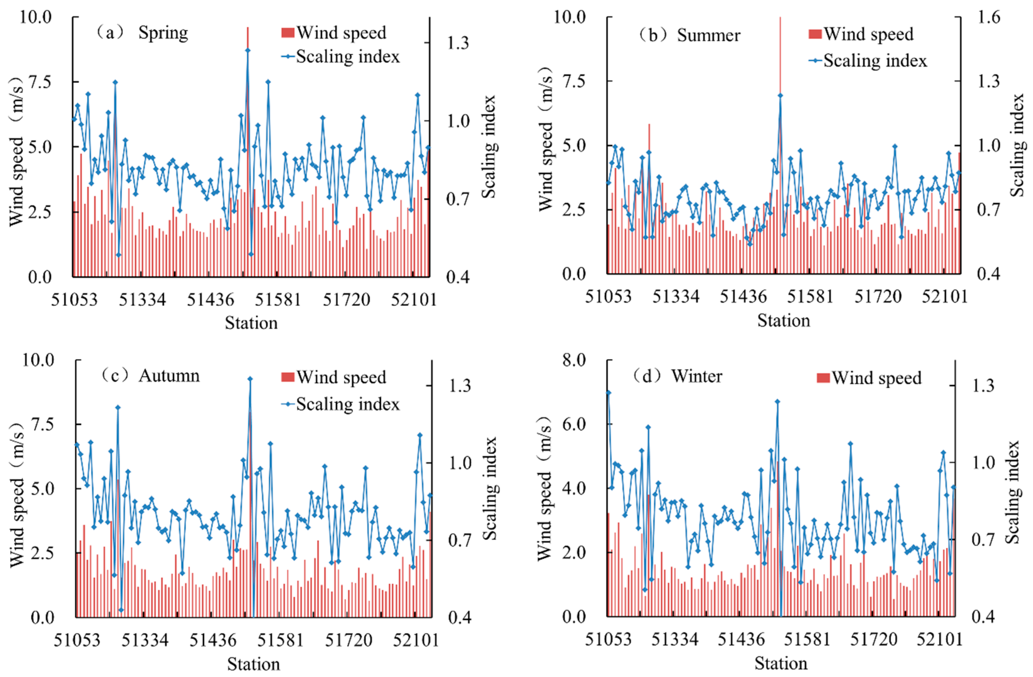
3.2. Characteristics of the Spatiotemporal Distribution
4. Discussion and Conclusions
Author Contributions
Funding
Institutional Review Board Statement
Informed Consent Statement
Data Availability Statement
Conflicts of Interest
References
- Zhang, H.; Peng, Y.X.; Niu, D. WRF simulation of near ground wind field in complex terrain regions. J. China Inst. Water Resour. Hydropower Res. 2018, 16, 98–104. (In Chinese) [Google Scholar]
- Xiong, M. Climate regionalization and characteristics of surface winds over China in recent 30 years. Plateau Meteorol. 2015, 34, 39–49, (In Chinese with an English Abstract). [Google Scholar]
- Liu, Y.; Li, H.; Ma, Z.; Xin, W. The nonlinear characteristics analysis of wind speed time series. J. North China Electr. Power Univ. 2008, 35, 99–102, (In Chinese with an English abstract). [Google Scholar]
- Li, Q.; Li, C.; Yang, Y. Application of wind speed self-similarity and fractal dimension in wind field analysis. Chin. J. Power Eng. 2016, 36, 914–919, (In Chinese with an English Abstract). [Google Scholar]
- Scarrott, C.; Macdonald, A. A review of extreme value threshold estimation and uncertainty quantification. REVSTAT 2012, 10, 33–60. [Google Scholar]
- Hu, X.; Fang, G.; Yang, J.; Zhao, L.; Ge, Y. Simplified models for uncertainty quantification of extreme events using Monte Carlo technique. Reliab. Eng. Syst. Saf. 2023, 230, 108935. [Google Scholar] [CrossRef]
- Li, Q.; Chen, L.; Zhang, Z.; Liu, W. Research on Long-Range Persistence of Tower Wind Speed Based on DFA Method. Meteorol. Sci. Technol. 2023, 51, 262–268, (In Chinese with an English Abstract). [Google Scholar]
- Lei, Y.D. Long-Term Persistence of Precipitation Sequences in Southern China. Master’s thesis, Nanjing University of Information Science and Technology, Nanjing, China, 2018. (In Chinese). [Google Scholar]
- Yuan, N.; Fu, Z.; Liu, S. Long-term memory in climate variability: A new look based on fractional integral techniques. J. Geophys. Res. Atmos. 2013, 118, 12–962. [Google Scholar] [CrossRef]
- Kavasseri, R.G.; Nagarajan, R. Evidence of crossover phenome-na in wind-speed data. IEEE Trans. Circuits Syst. 2004, 51, 2255–2262. [Google Scholar] [CrossRef]
- Kavasseri, R.; Nagarajan, R. A multifractal description of wind speed records. Chaos Solitons Fractals 2005, 24, 165–173. [Google Scholar] [CrossRef]
- Kavasseri, R.G.; Nagarajan, R. A qualitative description of boundary layer wind speed records. Fluct. Noise Lett. 2006, 6, 201–213. [Google Scholar] [CrossRef]
- Kocak, K. Examination of persistence properties of wind speed records using detrended fluctuation analysis. Energy 2009, 34, 1980–1985. [Google Scholar] [CrossRef]
- Telesca, L.; Lovallo, M.; Kanevski, M. Power spectrum and multifractal detrended fluctuation analysis of high-frequency wind measurements in mountainous regions. Appl. Energy 2016, 162, 1052–1601. [Google Scholar] [CrossRef]
- Li, Q.; Fu, Z.; Yuan, N.; Xie, F. Effects of non-stationarity on the magnitude and sign scaling in the multi-scale vertical ve-locity increment. Phys. A Stat. Mech. Appl. 2014, 410, 9–16. [Google Scholar] [CrossRef]
- Sun, B.; Yao, H.T. Multi-fractal detrended fluctuation analysis of wind speed time series in wind farm. CES Trans. Electr. Mach. Syst. 2014, 29, 204–210, (In Chinese with an English Abstract). [Google Scholar]
- Wang, X.; Mei, Y.; Li, W.; Kong, Y.; Cong, X. Influence of sub-daily variation on multi-fractal detrended fluctuation analysis of wind speed time series. PLoS ONE 2016, 11, e0146284. [Google Scholar] [CrossRef] [PubMed]
- Peng, C.K.; Buldyrev, S.V.; Havlin, S.; Simons, M.; Stanley, H.E.; Goldberger, A.L. Mosaic organization of DNA nucleotides. Phys. Rev. E 1994, 49, 1685. [Google Scholar] [CrossRef] [PubMed]
- Lei, Y.; Zhang, F.; Yang, Q.; Zhang, J.; Liu, R. Long-term memory behaviors for outgoing longwave radiation in the tropics. J. Trop. Meteorol. 2017, 33, 426–432, (In Chinese with an English Abstract). [Google Scholar]
- Zhao, S.; He, W. Evaluation of the performance of the Beijing Climate Centre Climate System Model1.1(m) to simulate precipitation across China based on long-range correlation characteristics. J. Geophys. Res. Atmos. 2015, 120, 12576–12588. [Google Scholar] [CrossRef]
- He, W.; Zhao, S.; Liu, Q.; Jiang, Y.; Deng, B. Long-range correlation in the drought and flood index from 1470 to 2000 in eastern China. Int. J. Climatol. 2016, 36, 1676–1685. [Google Scholar] [CrossRef]
- Yuan, N.; Ding, M.; Huang, Y.; Fu, Z.; Xoplaki, E.; Luterbacher, J. On the long-term climate memory in the surface air temperature records over Antarctica: A nonnegligible factor for trend evaluation. J. Clim. 2015, 28, 5922–5934. [Google Scholar] [CrossRef]
- He, W.; Zhao, S. Assessment of the quality of NCEP-2 and CFSR reanalysis daily temperature in China based on long-range correlation. Clim. Dyn. 2018, 50, 493–505. [Google Scholar] [CrossRef]
- Varotsos, C.; Kirk-Davidof, F.D. Long-memory processes in ozone and temperature variations at the region 60 S-60 N. Atmos. Chem. Phys. 2006, 6, 4093–4100. [Google Scholar] [CrossRef]
- Yuan, Q.; Yang, Y.; Li, C.; Kan, W.; Ye, K. Research of wind speed time series based on the Hurst exponent. Appl. Math. Mech. 2018, 39, 798–810, (In Chinese with an English Abstract). [Google Scholar]
- Jia, S.; Chen, X.; Song, Y.; Li, S. Analysis of characteristics of wind speed change in Xinjiang from 1970 to 2013. Ludong Univ. J. 2019, 35, 352–359, (In Chinese with an English Abstract). [Google Scholar]
- Tuniyazi, N.; Rezvagu, Z.; Meng, F.X. Analysis on forecasting of a winter gale in west of southern Xinjiang. Arid. Meteorol. 2018, 36, 1003–1011, (In Chinese with an English Abstract). [Google Scholar]
- Dong, K.H. Evaluation of Non-Stationary Wind and Its Impact on Structural Wind Loads. Master’s thesis, Beijing Jiaotong University, Beijing, China, 2015. (In Chinese). [Google Scholar]
- Tung, K.K.; Orlando, W.W. The k-3 and k-5/3 Energy Spectrum of Atmospheric Turbulence: Quasigeostrophic Two-Level Model Simulation. J. Atmos. Sci. 2003, 60, 824–835. [Google Scholar] [CrossRef]
- Shikhovtsev, A.Y.; Kovadlo, P.G. Estimation of mean energy characteristics of atmospheric turbulence at various heights from reanalysis data. Earth Environ. Sci. 2018, 211, 012023. [Google Scholar] [CrossRef]


| Season | Spring | Summer | Autumn | Winter | Whole Year |
|---|---|---|---|---|---|
| Scaling exponent | 0.92 | 0.75 | 0.91 | 0.94 | 0.91 |
| Wind speed (m/s) | 2.43 | 2.34 | 1.89 | 1.55 | 2.05 |
| Number of strong wind days (d) | 5.74 | 5.79 | 2.80 | 1.21 | 15.53 |
Disclaimer/Publisher’s Note: The statements, opinions and data contained in all publications are solely those of the individual author(s) and contributor(s) and not of MDPI and/or the editor(s). MDPI and/or the editor(s) disclaim responsibility for any injury to people or property resulting from any ideas, methods, instructions or products referred to in the content. |
© 2023 by the authors. Licensee MDPI, Basel, Switzerland. This article is an open access article distributed under the terms and conditions of the Creative Commons Attribution (CC BY) license (https://creativecommons.org/licenses/by/4.0/).
Share and Cite
Wang, X.; Lu, X.; Li, Q.; Zhou, H.; Li, C.; Zou, X. Study of the Characteristics of the Long-Term Persistence of Hourly Wind Speed in Xinjiang Based on Detrended Fluctuation Analysis. Atmosphere 2024, 15, 37. https://doi.org/10.3390/atmos15010037
Wang X, Lu X, Li Q, Zhou H, Li C, Zou X. Study of the Characteristics of the Long-Term Persistence of Hourly Wind Speed in Xinjiang Based on Detrended Fluctuation Analysis. Atmosphere. 2024; 15(1):37. https://doi.org/10.3390/atmos15010037
Chicago/Turabian StyleWang, Xiuqin, Xinyu Lu, Qinglei Li, Hongkui Zhou, Cheng Li, and Xiaohui Zou. 2024. "Study of the Characteristics of the Long-Term Persistence of Hourly Wind Speed in Xinjiang Based on Detrended Fluctuation Analysis" Atmosphere 15, no. 1: 37. https://doi.org/10.3390/atmos15010037