Testing Iron Stable Isotope Ratios as a Signature of Biomass Burning


Graduate School of Science, The University of Tokyo, 7-3-1 Hongo, Bunkyo, Tokyo 113-0033, Japan
*
Author to whom correspondence should be addressed.
Atmosphere 2019, 10(2), 76; https://doi.org/10.3390/atmos10020076
Submission received: 15 January 2019
/
Revised: 5 February 2019
/
Accepted: 7 February 2019
/
Published: 12 February 2019
(This article belongs to the Special Issue Air Quality in the Asia-Pacific Region)
Abstract
:Biomass burning is an important source of soluble Fe transported to the open ocean; however, its exact contribution remains unclear. Iron isotope ratios can be used as a tracer because Fe emitted by combustion can yield very low Fe isotope ratios due to isotope fractionation during evaporation processes. However, data on Fe isotope ratios of aerosol particles emitted during biomass burning are lacking. We collected size-fractionated aerosol samples before, during, and after a biomass burning event and compared their Fe isotope ratios. On the basis of the concentrations of several elements and Fe species, Fe emitted during the event mainly comprised suspended soil particles in all the size fractions. Iron isotope ratios of fine particles before and after the event were low due to the influence of other anthropogenic combustion sources, but they were closer to the crustal value during the event because of the influence of Fe from suspended soil. Although Fe isotope ratios of soluble Fe were also measured to reduce Fe from soil components, we did not find low isotope signals. Results suggested that Fe isotope ratios could not identify Fe emitted by biomass burning, and low Fe isotope ratios are found only when the combustion temperature is high enough for a sufficient amount of Fe to evaporate.
1. Introduction
Iron (Fe) in combustion aerosols emitted mainly by human activities exerts various effects on the environment and human health. The deficiency of dissolved Fe limits phytoplankton growth in some areas in the open ocean [1,2,3,4]. Since supply of Fe to the surface ocean stimulates primary production and affects carbon and nitrogen cycles, many studies have been conducted regarding Fe cycle in the ocean. The main sources of Fe to the surface ocean are natural aerosols (mainly aeolian dust), dissolution of coastal sediment, and hydrothermal vents [5], whereas Fe in combustion aerosols has been recognized as another possible Fe source due to its high solubility to seawater [6,7,8,9]. Although model studies estimate that approximately 30% of atmospheric soluble Fe deposition is from combustion sources, the relative contribution of natural and combustion aerosols to soluble Fe, especially in the open ocean, remains unclear [10].
Iron in combustion aerosols also contributes to enhancing the shortwave absorption of solar radiation. Iron emitted by anthropogenic combustions is mostly composed of aggregated nanoparticles of Fe oxides—such as magnetite, maghemite, and hematite—which are often observed in urban areas [11,12]. Iron oxides emitted by anthropogenic combustions are considered another important source for shortwave absorption, in addition to black and brown carbons [13].
Furthermore, Fe in combustion aerosols influences human health, which can enhance the production of reactive oxygen species that cause damage in vivo via the Fenton reaction [14]. Actually, magnetite nanoparticles were found in human brains, which possibly entered the brains directly via the olfactory bulb as insoluble particles and had a harmful effect on human health [15].
Therefore, the source, emission flux, solubility, and chemical/physical characteristics of Fe in various combustion aerosols should be clarified.
Iron stable isotope is an effective tool to distinguish the sources of Fe [5,16]. Iron isotope ratio (δ56Fe) is defined as
δ56Fe (‰) = 1000 × ((56Fe/54Fe)sample/(56Fe/54Fe)standard − 1),
Our previous studies analyzed Fe isotope ratios of size-fractionated aerosol particles near anthropogenic emission sources, which were collected in a tunnel, from an incinerator, and near a steel plant. We found that δ56Fe values of Fe emitted during the combustion processes ranged from −1‰ to −4‰ [17,18,19], which were much lower than those of terrestrial igneous rocks (0.00 ± 0.10‰, [20]) and other natural materials [21]. The remarkably low δ56Fe values were possibly caused by isotope fractionation during evaporation under high-temperature condition. The low δ56Fe values can be used to estimate the contribution of Fe of combustion aerosols within total aerosol particles.
Among various combustion sources, biomass burning—such as forest fires, savanna or grassland fires, and crop residue burning—are considered one of the main Fe emission sources [8,22]. In a model study, its contribution is estimated to be approximately half of total soluble Fe deposition in a part of the southern hemisphere, where biomass burning is considered a dominant Fe source compared with mineral dust and fuel combustion [8]. Although biomass burning can increase atmospheric Fe concentration in the regional scale, the concentration is not higher than Fe emission due to dust events [22,23,24]. Iron from biomass burning is important due to its high solubility, which is enhanced during its transportation mixed with organic matters emitted by biomass burning [23,24].
On the basis of our previous studies on Fe isotope ratios, it is possible that Fe emitted by biomass burning also has low δ56Fe values due to isotope fractionation during combustion. Given that combustion temperature of biomass burning is possibly lower than those of other anthropogenic sources, Fe amount emitted via evaporation can be small. However, the extent of isotope fractionation differs not only by temperature but also by many factors, such as vapor pressure in each system, other coexistent components, Fe species, and so on. [25,26] Therefore, it is unknown whether Fe isotope fractionation is large enough to be observed in actual aerosol particles or not. In addition, some plants originally have δ56Fe values as low as −1.6‰ [27], which can be reflected in biomass-derived aerosol particles. However, data on δ56Fe values of aerosols emitted by biomass burning have not been reported. A previous study suggested that low δ56Fe values detected in fine aerosol samples may be derived from biomass burning, although strong evidence to support the presence of particles originating from biomass burning is unavailable [28].
We chose a reed burning event held once in a year at Watarase control basin in Tochigi as an observation site. This reed burning is one kind of grassland fire. Although reed burning is not a popular type of burning [29,30], the burned area (approximately 15 km2) at a time is especially large in Japan. Therefore, it is expected that emission from biomass burning is clearly observed with little influence from other sources.
This study aimed to investigate whether isotope fractionation can be practically observed in aerosols emitted during biomass burning and if the isotope ratio can be used as a tracer to estimate the contribution of biomass burning in aerosols. We collected size-fractionated particles emitted before, during, and after a biomass burning event. For this purpose, we estimated sources of particles by comparing concentrations of major ions and some elements. Iron solubility and Fe species were also examined to characterize Fe in particles collected before, during, and after the event. Considering the differences in Fe isotope ratios among the sample sets, we discussed whether Fe isotope ratio may be used to quantify the amount of Fe emitted by biomass burning.
2. Experiments
2.1. Sampling
Aerosol particles emitted by the biomass burning event were collected on the roofs of Oyama City Office (36.3149° N, 139.8001° E, approximately 15 m above the ground) and Shimonamai Elementary School (36.2473° N, 139.7091° E, approximately 10 m above the ground) during a reed (Phragmites australis) burning event which is held once a year in March at Watarase Basin, Tochigi, Japan (36.1° N, 139.4° E). Oyama City Office and Shimonamai Elementary School are approximately 12 and 1 km to the northeast from Watarase Basin, respectively (Figure 1). Since southwest wind is predominant in this area in March, it was expected that emission from the burning event can be observed in both sampling points [31]. Furthermore, Shimonamai Elementary School is surrounded by the basin, thus, aerosol particles emitted from the burning event can be collected in any wind direction. We refer to Oyama City Office and Shimonamai Elementary School as the ‘12 km site’ and ‘1 km site’, respectively. Sample collections were conducted before, during, and after the event at the 12 km site, but only during the event at the 1 km site (Table 1). Aerosol particles were collected on filters using a high-volume air sampler (Kimoto, MODEL-123, Osaka) with a cascade impactor (Tisch Environmental Inc., Series 230), and particles were separated into seven size fractions (stage 1, >10.2 μm; stage 2, 4.2–10.2 μm; stage 3, 2.1–4.2 μm; stage 4, 1.3–2.1 μm; stage 5, 0.69–1.3 μm; stage 6, 0.39–0.69 μm; backup filter (BF), <0.39 μm). To minimize contamination from filter materials, PTFE sheets (Naflon tape; thickness: 0.2 mm; Nichias Co., Ltd., Tokyo, Japan) were cut into a suitable form for stages 1–6, details of which is described in Sakata et al. [32]. For BF, ADVANTEC PF050 PTFE filter was used. The PTFE filters for stages 1–6 were washed by 3 M HNO3, 3 M HCl, and ultrapure water without heating for one day, respectively. Soil and reeds in the Watarase Basin were also collected to compare their Fe isotope ratios with those in the aerosol samples.
2.2. Acid Digestion and Leaching Experiments
Concentrations of Fe, aluminum (Al), titanium (Ti), zinc (Zn), and lead (Pb) were analyzed using inductively coupled plasma mass spectrometry (ICP-MS; Agilent 7700, Tokyo, Japan). Filter digestions were conducted under HEPA-filtered environment (SS-MAC 15, Air Tech, Tokyo, Japan). All equipment was preliminarily washed with acid. Aerosol samples were digested with mixed acids (HNO3, HCl, and HF, Tamapure AA-100, Tama Chemicals, Kawasaki, Japan), details of which are described in Kurisu et al. [19]. Concentrations of these elements in washed PTFE and unwashed PF050 were subtracted from their concentrations in each sample. The Fe concentrations of the washed PTFE sheet and PF050 filter in this study were 6.7 ± 4.8 ng Fe/cm2 sheet and 55 ± 44 ng Fe/cm2 filter, respectively, which were less than 1% of Fe in aerosol particles collected before and after the event, respectively, but less than 10% and 30% for PTFE and PF050 filters, respectively, during the event. The larger blank ratios than those before and after the event were due to the shorter sampling durations. Reed was washed by ultrapure water via ultrasonic treatment and dried before decomposition to remove soil attached to the reed. Reed was decomposed with 2 mL of 15.2 mol/L HNO3 and 1 mL of 11.7 mol/L H2O2 after the same procedure was employed for the aerosol samples to decompose remaining organic matters completely.
Major ions (Cl−, NO3−, SO42−, C2O42−, Na+, NH4+, K+, Mg2+, and Ca2+) were analyzed through ion chromatography (Dionex, ICS-1100). In addition, the concentration of water-soluble Fe was measured by ICP-MS. For these analyses, approximately 1/40–1/20 of a filter (3–6 cm2) was soaked in 15 mL of ultrapure water over night after ultrasonic treatment for 30 min. Columns and eluent compositions for ion chromatography were the same as those employed by Kurisu et al. [18] Non-sea-salt (nss) SO42− and K+ were calculated according to the equations
where 0.25 and 0.037 are the weight ratios of SO42−/Na+ and K+/Na+ in seawater, respectively [33].
nss-SO42− = [SO42−] − [Na+] × 0.25,
nss-K+ = [K+] − [Na+] × 0.037,
Fractional Fe solubility was calculated as
fractional Fe solubility (%) = 100 × ([Fe]water-extracted/[Fe]total)
2.3. X-Ray Absorption Fine Structure (XAFS) Analysis
Iron species of aerosol samples and soil were determined by XAFS analysis. X-ray absorption near-edge structure (XANES) spectra of bulk aerosol particles in each size fraction and soil were analyzed at the beamline BL-12C of Photon Factory (PF), KEK (Ibaraki, Japan) and BL01B1 of SPring-8 (Hyogo, Japan). Spot analysis of aerosol samples was also conducted by μ-XRF-XAFS at the BL-4A of PF. Methods were the same as those reported by Kurisu et al. [19].
2.4. Scanning Transmission X-Ray Microscope (STXM) Analysis
Carbon K-edge XANES spectra were obtained by STXM at the BL-13A of PF [37]. Carbon XANES spectra of black carbon (biochar) emitted by biomass burning can change by temperature. Keiluweit et al. [38] investigated changes in C spectra by heating grass at different temperatures (0–700 °C) for 1 h. Although original C component in reed may be different from that of grass in Keiluweit et al., characteristics of spectral change are basically consistent among various plants [39]. Therefore, their results could be adopted to estimate rough combustion temperature in this study. Aerosol particles at stage 6 of the 1 km site sample during the event collected on a molybdenum TEM grid were analyzed.
2.5. Iron Isotope Analysis
Iron isotope analysis was conducted by multicollector-ICP-MS (MC-ICP-MS, Neptune Plus, Thermo Fisher Scientific, Bremen, Germany). Decomposed aerosol samples for ICP-MS analysis were evaporated nearly to dryness and dissolved into 2 mL of a mixture of 6 mol/L HCl and 0.3 mmol/L H2O2 for Fe separation with Bio-Rad AG MP-1 (100–200 mesh) anion exchange resin. A sample was loaded into a column (Poly Prep Chromatography Columns, Bio-Rad) filled with 0.6 mL of the resin after washing and conditioning. Then 2 mL of a mixture of 6 mol/L HCl and 0.3 mmol/L H2O2 was loaded into the column five times to remove interference elements including chromium and copper (Cu). Subsequently, Fe was collected into a perfluoroalkoxy alkanes (15 mL) vial by loading 2 mL of a mixture of 0.5 mol/L HCl and 0.3 mmol/L H2O2 four times. The solution was evaporated nearly to dryness, redissolved into 0.2 mL of 15 mol/L HNO3, and heated at 150 °C for several hours to decompose remaining organic matters. After evaporation, it was redissolved into appropriate amount of 0.3 mol/L HNO3 so that Fe concentration became 500 μg/L for isotope analysis. Copper solution (Wako Pure Chemical Industries., Osaka, Japan) was added to the Fe fraction so that Cu concentration became 200 μg/L. Average Fe recovery was 95±12%, meaning that almost no isotope fractionation occurred during the column separation.
Faraday cup setting of MC-ICP-MS is the same as Kurisu et al. [18]. Medium resolution mode was adopted to separate Fe signals from molecular ions, such as argon oxide and nitride. A quartz spray chamber was used for sample introduction and Ni sampling and skimmer cones were employed at the interface. Typical intensity of 56Fe was 2.5–3 V. For mass bias correction with Cu isotope ratio, exponential law was used [40]. Bracketing solution (IRMM-014) was measured before and after each sample measurement with 60 cycles in each set of measurement, and average value of the two bracketing measurements was used for calculation with Equation (1). An error (2 standard error, 2σ) for a single sample analysis was calculated as
where σsamp, σstd1, and σstd2 represent standard errors of a sample and bracketing before and after the sample, respectively.
2σ = 2 × {σsamp2 + (σstd12 + σstd22)/4}1/2
An average δ56Fe value for repeated analyses of standard granite materials (JB-2, Geochemical reference samples, Geological Survey of Japan) was 0.11 ± 0.14‰ (2 standard deviation, n = 13), which was consistent with a previous report (0.06 ± 0.03‰, [41]).
We also analyzed soil, reed, and residual ash. Given the difficulty in distinguishing between residual ash and soil in Watarase Basin, ash was produced by heating reed in a tube furnace (TMF-500N, ASONE, Tokyo, Japan) under ambient air conditions at 400–500 °C for 7–9 h. Iron isotope ratios of soluble Fe at stage 6 were also analyzed. For extraction, simulated rainwater (RW, 0.020 mol/L oxalic acid/ammonium oxalate at pH 4.7) was used instead of ultrapure water because the amount of extracted Fe by ultrapure water was too small for isotope analysis.
3. Results
3.1. Characteristics of Aerosols
3.1.1. Concentrations of PM2.5, Major Ions, Fe, and Other Trace Elements
Hourly concentration data of PM2.5 at Oyama City Office were obtained from Atmospheric Environmental Regional Information System (Figure 2) [42]. The concentrations of PM2.5 was clearly high during the reed burning event (26 March, 8 a.m. to 5 p.m.), thereby suggesting that the aerosol samples during the event were greatly influenced by particles emitted by the burning event.
To discuss different characteristics of aerosols during the event and non-event, concentrations of each component were averaged over (i) the 1 km and 12 km site during the event (referred as the event) and (ii) the 12 km site before and after the event (referred as the non-event).
Major ion concentrations (Cl−, NO3−, C2O42−, SO42−, Na+, NH4+, K+, Mg2+, and Ca2+) showed certain characteristics during the event at stage BF (Figure 3). Concentrations of the measured ions of the event sample were similar or lower compared with the non-event sample, except for stage BF (<0.39 μm). The concentrations of Cl−, NO3−, C2O42−, NH4+, K+, Mg2+, and Ca2+ at stage BF were much higher than the non-event. This result suggested that a large number of submicron particles were emitted by the burning event. C2O42− was not detected in coarse particles of the non-event sample, but it was detected in the event sample, which supported the large influence of the burning event, as was also suggested in previous studies [23,24,43,44]. The NO3- concentration was higher than the non-event at stage BF, but that of nss-SO42− was lower, which may be derived from higher NOx/SOx emission ratio from biomass burning than that from other anthropogenic sources [43,45].
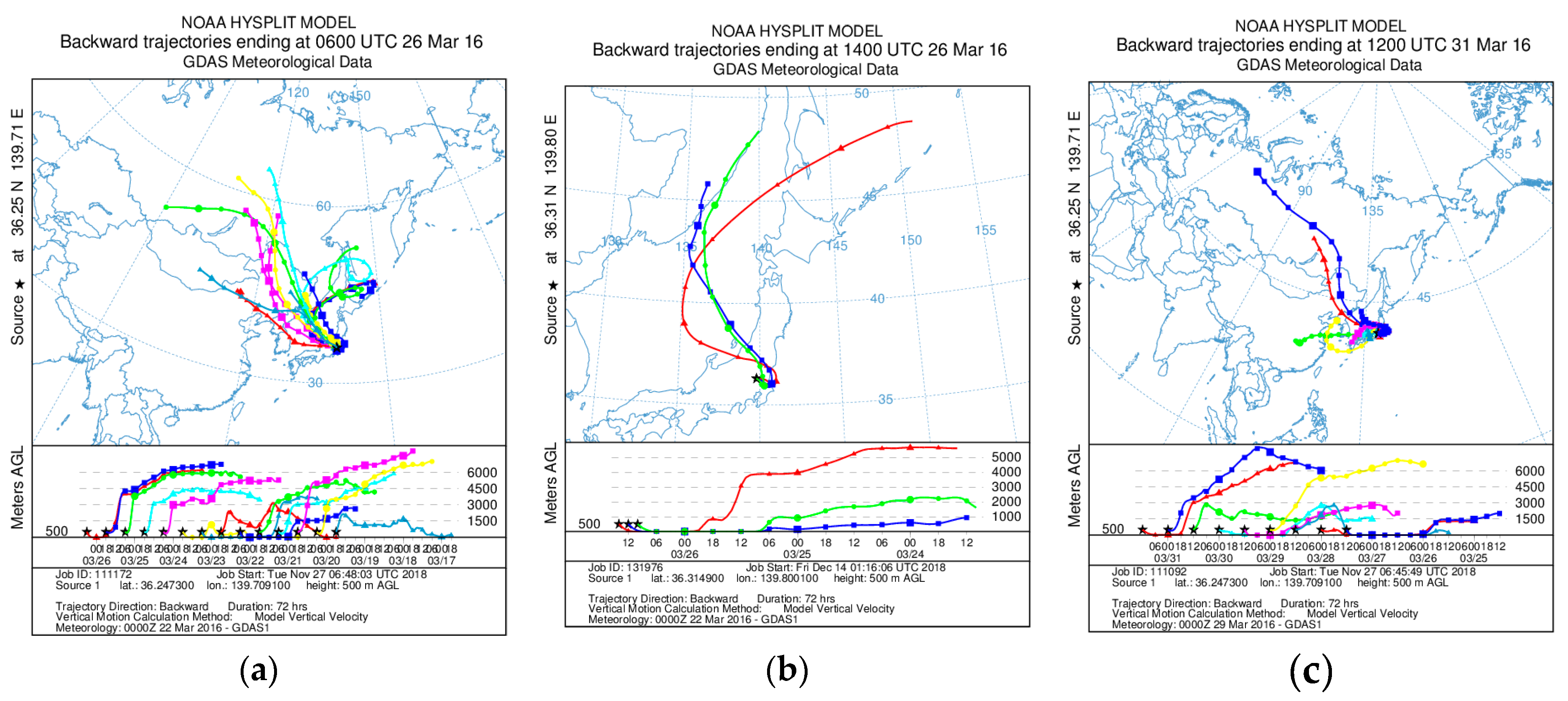
Concentrations of K, Al, Ti, Fe, Zn, and Pb in Watarase soil, reed, and various plants are shown in Table 2. Concentration of K, which is often used as a tracer of biomass burning [23,24,30,43,46], was high in reed and various plants. Concentrations of crustal-abundant elements including Fe, Al, and Ti in reed and various plants were lower than those in the soil. Concentrations of Zn and Pb, often used as tracers of fuel combustion [47], were also lower in reed and plants than in the soil. However, sometimes Zn is enriched in biomass-derived aerosols [46,48], possibly due to high volatility and higher concentrations compared with other volatile elements such as Pb. Based on these results, we characterized the aerosol samples. At stages 1–6, size distributions of concentrations of measured elements including Al, Ti, Fe, Zn, and Pb of the event sample were basically similar to those of the non-event sample (Figure 4). By contrast, at stage BF (<0.39 μm) during the event, the concentrations of Al, Ti, and Fe were higher than those of the non-event (Figure 4). These results suggested that fine particles containing these elements (Al, Ti, and Fe) were emitted by the burning event. Although we do not know the exact reason for the high concentrations of crustal-abundant elements (Al, Ti, and Fe) at stage BF even in the non-event sample, they may be due to the long-range transportation of Kosa dust [49], which is also supported by the air masses coming from the Asian continent (Appendix A). High Zn concentration at stage BF during the event was attributable to biomass combustion [46].
Enrichment factors (EFs) of Ti, Fe, Zn, and Pb were calculated with the equation
where M is a target element, and M/Al is the concentration ratio of M and Al (Figure 5). (M/Al)sample values were normalized to those of soils collected at Watarase Basin (Table 2). EFFe values of the non-event were in the range of 1.5–2.0, with the highest value at stage 6 (0.39–0.69 μm). Considering that Fe/Al of crustal average (0.68) is higher than that of Watarase soil (0.51) [52], EFFe values slightly higher than 1 indicated that they were mainly transported from other regions than Watarase Basin, possibly from the Asian continent. During the event, EFFe values were closer to 1, even at stage BF (<0.39 μm), where Fe concentrations were especially high. Since Fe/Al ratios of reed and residual ash were 0.83 and 0.87, respectively, they were not responsible for the lower EFFe values in the event sample than those in the non-event sample. These results demonstrated that Fe was influenced by Watarase soil even in fine particles. Titanium, a crustal abundant element, also showed EFTi values close to 1, which supported the influence of soil particles. EFZn and EFPb were much higher than 1 in fine particles in both of the samples. As Zn and Pb in fine particles are mainly emitted by fuel combustion [47], the samples in this study were also constantly influenced by such anthropogenic combustion. EFZn and EFPb values in the event sample were lower than those in the non-event sample (but still much higher than 1), which could be caused by a large amount of Al derived from soil. Although the Zn concentration of the event sample was high possibly due to biomass combustion, higher levels of EFZn were not observed, thereby suggesting the strong influence of Al derived from soil.
EFM = (M/Al)sample/(M/Al)soil,
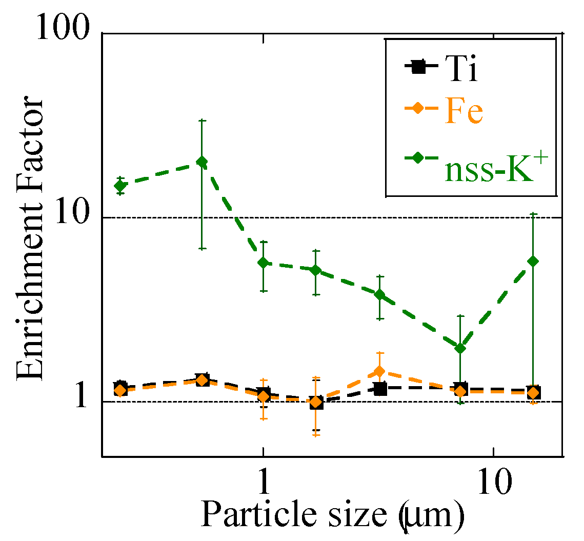
To determine the influence of the burning event, we discussed the nss-K+ concentration, an indicator of emission from biomass burning [53]. Given that K+ is also present in soils, we also calculated EFK+ values and compared them with EFFe and EFTi values of the event sample (Figure 6). nss-K+ concentrations in both of the samples were higher in finer particles than in coarse particles (Figure 3j). The concentration was the higher during the event at stage BF (0.39 μm), suggesting that a large numbers of K+-containing particles were emitted by the event (Figure 3j). EFK+ values were much higher than 1, especially in fine particles, despite that EFFe and EFTi values were close to 1 for all the size fractions. Hence, although a large number of biomass-derived particles were emitted by the event, Fe was largely influenced by soil particles, not biomass.
Large influence of Fe from soil particles was also suggested from Fe species by XAFS analysis, in which the proportions of Fe in silicate minerals in fine particles were larger during the event than those before and after the event. The result is explained in detail in the Appendix B.
3.1.2. Fractional Fe Solubility
Fractional Fe solubilities were less than 1% for all the coarse particles (Figure 7), and this finding was presumably derived from Fe in dust particles with fractional Fe solubility lower than 1% [9,54]. In fine particles, fractional Fe solubilities of the non-event sample increased up to 6% at stage 6 (0.39–0.69 μm). EFZn and EFPb were especially high at stage 6 before and after the event; thus, the increased fractional Fe solubilities of fine particles were considered to be due to large amounts of anthropogenic combustion aerosols with increased Fe solubility, as is usually observed in urban aerosols [6,7,8,9]. During the event, fractional Fe solubilities of fine particles were lower (0.6–1.7%) than those before and after the event and not extremely different from those of coarse particles in the same samples. This fractional solubility was presumably caused by large influence of Fe from suspended soil.
3.1.3. Estimation of Combustion Temperature from C K-edge XANES
Carbon K-edge XANES spectra of several particles at stage 6 (0.39–0.69 μm) at the 1 km site during the event were obtained (Figure 8). According to Keiluweit et al. [38], the peak of C=C aromatic bond (around 285–286 eV) increase, whereas the peaks of other functional groups (e.g., carboxyl C–OOH around 288.6 eV and C–O around 289.2 eV) decrease as the combustion temperature increases [38]. In the spectra of the present study, the peak height around 288.6 eV of each spectrum was almost similar or higher than that at 285–286 eV, which were close to the spectra of grass combusted at 300–500 °C. Therefore, the samples were combusted under this temperature range.
3.2. Iron Isotope Ratios
3.2.1. Soil, Reed, and Residual Ash
As possible sources of aerosol particles during the event, δ56Fe values of soil, reed, and residual ash were analyzed and we found that the average values were +0.04 ± 0.20‰, +0.08 ± 0.10‰, and +0.09 ± 0.03‰, respectively. No difference was found between reed and residual ash, thereby indicating minimal fractionation between them. We then compared the Fe/Al concentration ratios of reed and residual ash, considering that most Al remains in ash due to high refractoriness. The Fe/Al weight ratio in residual ash was 90 ± 10% of that in original reed. The ratio of the residual ash being slightly lower than that of reed suggests that approximately 10% of Fe in reed could evaporate. We did not measure the δ56Fe values of the evaporated Fe, but the evaporated Fe possibly had low δ56Fe values. This finding needs further investigation.
No difference was noted between reed and soil. Grass absorbs Fe by chelating Fe(III) in soil, and little or no isotope fractionation occurred between Fe in reed and soil [27].
3.2.2. Bulk Aerosol
Before and after the burning event, coarse particles (>1 μm) of all the samples had similar δ56Fe values (on average 0.04 ± 0.08‰), which were close to those of Watarase soil (+0.04 ± 0.20‰), reed (+0.08 ± 0.10‰), residual ash (+0.09 ± 0.03‰), and reported terrestrial igneous rocks (0.00 ± 0.05‰, Figure 9) [20]. Fine particles (<1 μm) yielded δ56Fe values lower than those of coarse particles, especially at stage 6 (0.39–0.69 μm; −1.06 ± 0.12‰ and −1.26 ± 0.13‰ before and after the event, respectively). The low δ56Fe values in fine particles before and after the event were presumably because of particles originated from anthropogenic combustion, which was suggested from the high EF values of Zn or Pb, trace elements emitted by fuel combustion. These size distributions of δ56Fe values were similar to those observed in Higashi-Hiroshima (suburban environment in Japan) [18], thereby suggesting that the distribution is a typical pattern in these areas where aerosols originated from anthropogenic and natural materials.
During the event, the δ56Fe values of coarse particles were identical to those before and after the event (on average 0.01 ± 0.17‰), and fine particles yielded lower δ56Fe values (−0.61 ± 0.13‰ and −0.36 ± 0.08‰ for stage 6 of the 12 and 1 km sites, respectively) than coarse particles. However, the values in fine particles were clearly higher than those before and after the event. Furthermore, the δ56Fe values of fine particles were higher at the 1 km site than at the 12 km site, indicating that Fe emission from the burning event had high δ56Fe values. Considering that EFFe values during the event were close to 1 and large amount of Fe originated from silicate minerals were noted during the event, Fe from Watarase soil with δ56Fe value close to 0‰ was suspended and collected as aerosol particles. This procedure caused the δ56Fe values to be higher than those obtained before and after the event.
3.2.3. Soluble Fe Fraction of Aerosols
Most of Fe in aerosol particles were of soil origin, as was suggested in the previous sections. To evaluate δ56Fe values of combustion aerosols including evaporated Fe by the burning event and other anthropogenic Fe, the δ56Fe of extracted Fe at stage 6 was measured, considering that Fe in combustion aerosols are more soluble than Fe in soil [9,54]. Simulated RW (0.020 mol/L oxalic acid/ammonium oxalate at pH 4.7) extracts larger amount of Fe sufficient for isotope analysis compared with ultrapure water; however, simulated RW still extracts Fe (hydr)oxides preferentially compared with silicate minerals [7]. Most of the Fe in combustion aerosols is Fe (hydr)oxide, hence, its influence could be observed clearly, although quantitative evaluation of the δ56Fe values of combustion aerosols are difficult due to the coexistence of Fe (hydr)oxides in soil.
Before the event, δ56Fe values of soluble Fe at stage 6 (0.39–0.69 μm) were lower than those of total Fe (Figure 10). This result was similar to our previous results in Higashi-Hiroshima, thereby indicating that anthropogenic Fe with low δ56Fe values was preferentially extracted [18]. During the event, the δ56Fe values of soluble Fe were similar or slightly lower than those of total Fe at each site, and the difference between soluble and total Fe was smaller than that before the event. This smaller difference is partially because of dissolution of soil-derived Fe (hydr)oxides, but we did not find a clear sign of low δ56Fe values even in the soluble fraction. Thus, biomass burning is not an important source of Fe with very low δ56Fe values. It should be noted the δ56Fe values of soluble Fe after the event, in addition to the samples during the event, did not change to a large degree. We did not examine the clear reason for these similarities, but Fe emitted by the event was partially present in the sample after the event, which was supported by the slightly higher PM2.5 concentrations after the event than before the event (Figure 2). Therefore, soluble Fe possibly contained a high amount of soil-derived Fe (mainly (hydr)oxides) after the event.
4. Discussion
4.1. Atmospheric Concentration and Fractional Solubility of Fe Emitted by Biomass Burning
In this study, high Fe concentration during the event was not observed except for stage BF (<0.39 μm). Iron emitted during the event mostly originated from suspended soil regardless of particle size, which was suggested from EFFe values and Fe species. Soil suspension was enhanced by convection during biomass burning [55].
The burning event in this study was caused by the combustion of reed. However, many other kinds of biomass burnings exist, such as forest fires, savanna, or grassland fires, and burning of crop residue [29,30]. Therefore, characteristics of emitted materials can differ among various kinds of fires or burned plants, and the amount of suspended soil varies depending on burning conditions, such as vegetation, density of vegetation (high density of vegetation can cover soils and suppress their suspension), and wetness of soils [56]. Iron concentration in plants also differ depending on plant species and soil conditions (Table 2, [51]). Nevertheless, similar results have been observed in other studies focusing on other kinds of biomass burnings [23,24,57]. Paris et al. [23] collected aerosol samples during African savannah fire season and suggested that Fe concentrations during that time were lower than those during the dust event; whereas high influence of soil during biomass burning was observed based on similar Fe/Al ratios between dust and biomass burning periods. Siefert et al. [57] also collected aerosols during forest fire events in Pasadena and suggested the influence of Fe from soil suspension. Therefore, Fe from soil rather than Fe from biomass combustion is presumably crucial in aerosols emitted by numerous biomass burnings.
Fractional Fe solubilities in fine particles were lower during the event than before and after the event. This is possibly due to the large amount of soil-derived Fe with low solubility in fine particles, and this finding was consistent with the results of EFFe and Fe species. Iron emitted by biomass burning becomes highly soluble during transportation by interacting mainly with organic matters, such as oxalate, in biomass-burning aerosols [8,23,24]. The sampling points in this study were close to the emission source, thus, high fractional Fe solubility caused by the reactions during such transportation was not observed, as was the case for other studies [24]. Although our results suggested that Fe emitted by the burning event was not an important soluble Fe source near the emission site, the solubility of Fe (mainly of soil origin) possibly increases during transportation and becomes an important soluble Fe source to the open ocean.
4.2. Can Low δ56Fe Values Be Used as a Tracer of Biomass Burning?
The δ56Fe values at stage 6 (0.39–0.69 μm) during the event were higher than those before and after the event, thereby indicating the influence of Fe from soil, as described in Section 3.2.2. However, the values were still lower than those of coarse particles, possibly because some particles with low δ56Fe values were mixed with soil particles. We discuss the possible sources of these particles with low δ56Fe values to clarify if they are signals related to the burning event. Possible sources of aerosol particles other than soils are reed, residual ash, evaporated Fe by biomass burning, and similar anthropogenic Fe detected before and after the event. Reed and residual ash were not possible sources for the low δ56Fe values because their δ56Fe values were close to 0‰. The evaporation of Fe during the burning event could be a reason for the low δ56Fe values, if Fe isotope fractionation occurred during evaporation [17,18,19]. We calculated the possible amount of Fe evaporated by the burning event on the basis of the concentrations of Fe and K in aerosols and reed. The concentrations of total K (decomposed by mixed acid and measured by ICP-MS) and Fe at stage 6 of the 1 km site were 64 and 30 ng/m3, respectively. Since concentrations of Fe and K in reed were 0.013 wt % and 0.26 wt %, respectively (Table 2), the Fe/K weight ratio in reed in this study was approximately 0.05. In addition, amount of evaporated Fe is approximately 10% of total Fe in reed, on the basis of the result of comparison of the Fe/Al weight ratio between reed and residual ash in Section 3.2.1. In this case, the ratio of evaporated Fe and K from reed is approximately 0.005, assuming that most of K in reed is evaporated. Even if all K at stage 6 of the 1 km site is of reed origin, the evaporated Fe concentration is less than 0.32 ng/m3, which is approximately 1% of total Fe at stage 6 (30 ng/m3). Assuming that (i) the δ56Fe value of evaporated Fe fraction is as low as −4.7‰ based on our previous studies [17,18,19], and (ii) the δ56Fe value of the other Fe sources is 0.0‰, the δ56Fe value of the aerosol sample becomes −0.047‰, which cannot explain the observed δ56Fe value (−0.36 ± 0.08‰). Therefore, evaporation of Fe during the burning event was not a possible Fe source for the observed δ56Fe value. Considering that the Fe concentration at stage 6 during the event was similar to that of the non-event sample, the external Fe was possibly from any anthropogenic sources similarly observed before and after the event, which contributed to the low δ56Fe values during the event.
Thus, the Fe isotope ratio was difficult to use for distinguishing Fe emitted by biomass burning from Fe in mineral dust. Some of the plants may originally have negative δ56Fe values [27]. However, the values cannot be reflected in aerosol particles because soil-derived Fe is predominant in most observed biomass burnings [23,24]. Further studies are necessary to verify these findings.
4.3. Fe Isotope Fractionation During Combustion
In this study, we did not find low Fe isotope signals from biomass burning mainly because of the influence of suspended soil emitted during biomass burning. Moreover, we measured the δ56Fe values of soluble Fe fraction to reduce the influence of soil, in which we did not find low δ56Fe due to biomass burning. The samples were influenced constantly by human activities, such as fuel combustion, as was suggested from high EFPb values, which made detecting clearly low δ56Fe values due to biomass burning difficult. Given that the Fe/Al ratio of residual ash was lower than that of reed, some amount of Fe possibly evaporated during combustion. Therefore, further investigation such as combustion experiments are necessary to clarify Fe isotope fractionation process during biomass burning.
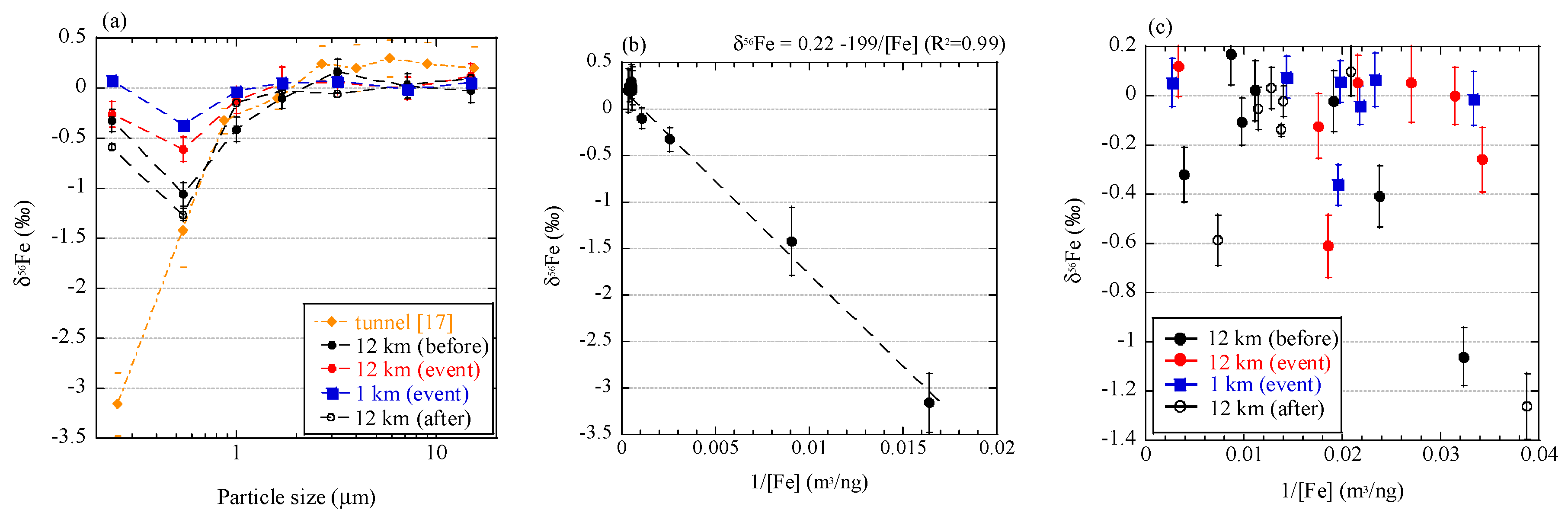
To discuss the relationship of Fe isotope fractionation and combustion processes, we compared the results in this study with those of aerosol particles originating from vehicle emission [17]. Fine aerosol particles collected in a tunnel showed δ56Fe values up to 3.5‰ lower than those of coarse particles (Figure 11a). This sampling was conducted in a tunnel where approximately 38,000 vehicles pass daily. No particular source of low δ56Fe values was found except for combustion in vehicles. We noted that a good correlation between δ56Fe value and inverse of Fe concentration of each size fraction, when a considerable amount of Fe was emitted by the combustion (Figure 11b). However, such a correlation was not found in aerosols collected in the present study (Figure 11c). The correlation in the tunnel indicated that Fe was derived from two different sources, and the δ56Fe values were explained by mixing the two sources [19]. In the case of the particles in the tunnel, one source was crustal materials with δ56Fe values close to 0.22‰ (intercept of the correlation line) and the other source was isotope-fractionated particles with δ56Fe values lower than −3.2‰ (the lowest value of aerosol particles). The Fe with low δ56Fe values may be derived from Fe nanoparticles emitted from the cylinder engines, where temperature exceeds 2200 °C [58]. In such high temperature, Fe can partially evaporate because the vapor pressure of Fe increases around 2200 °C (Appendix C, [59]). Therefore, evaporation during combustion in vehicles occurred and was accompanied with emission of particles with low δ56Fe values. Furthermore, Fe was the main component in the source materials (i.e. cylinder engine), which allows the emission of a considerable amount of evaporated Fe, in spite of partial evaporation. On the other hand, C K-edge XANES analysis revealed that the combustion temperature of the burning event was approximately 300–500 °C, which was possibly too low for any considerable amount of Fe to evaporate. Iron may evaporate at low temperatures as more volatile Fe species, such as Fe chloride. However, the temperature was still too low for significant amount of Fe chloride to evaporate (Appendix C). In addition, the Fe content in reed was small compared with Fe emission from soil, as discussed in Section 4.2. Therefore, the amount of Fe evaporated by biomass burning was low.
Low δ56Fe values due to evaporation should be observed only when (i) Fe content in original materials is high and (ii) the combustion temperature is high enough to produce a sufficient amount of evaporated Fe. Such high temperature conditions are basically limited to anthropogenic sources, such as engine combustion, fuel combustion, and metal manufacturing. Although the difference in the degree of Fe isotope fractionation among these anthropogenic sources remains unknown, they yield approximately −3.9‰ to −4.7‰ [17,18,19]. The extent of evaporation and δ56Fe values are determined by many factors, such as temperature, vapor pressure in each system, other coexistent elements, viscosity of Fe in solid or liquid phase, and Fe species [25,26]. It should be pointed out that volcano activities have possibly high temperatures that are enough to evaporate Fe [60], and Fe emitted by volcanoes may have low δ56Fe values; however, no reports have been made on this process. Further studies on Fe isotope fractionation during combustion are necessary to know how to employ low δ56Fe values as a tracer of evaporated Fe from various combustion sources.
5. Conclusions
This study focused on Fe isotope ratios of particles emitted by biomass burning to investigate Fe isotope fractionation during combustion and determine if Fe isotope ratios can be used as tracers of Fe aerosol particles from biomass burning. Most Fe particles were derived from suspended soil, which made δ56Fe values of fine particles during the burning event higher than those before and after the event. We did not find clear signals of Fe isotope fractionation during the burning event, possibly because of the lower combustion temperature compared with other anthropogenic combustion processes. Therefore, low δ56Fe values could not be used as a tracer for biomass burning but as a tracer of human activities including high-temperature processes.
Author Contributions
Conceptualization, M.K. and Y.T.; Data curation, M.K.; Formal analysis, M.K.; Funding acquisition, M.K. and Y.T.; Investigation, M.K. and Y.T.; Methodology, M.K. and Y.T.; Project administration, Y.T.; Resources, Y.T.; Supervision, Y.T.; Validation, M.K., and Y.T.; Visualization, M.K.; Writing—original draft, M.K.; Writing—review & editing, Y.T.
Funding
This research was funded by Grant-in-Aid for JSPS Research Fellow grant number 17J06716, Grant-in-Aid for Scientific Research (A) grant number 18H04134, and Grant-in-Aid for Challenging Exploratory Research grant number 16K13911.
Acknowledgments
We appreciate staffs in Oyama City Office and Shimonamai elementary school for the cooperation for the sampling. We are grateful to Kohei Sakata and Yasuo Takeichi for technical support with experiments. XAFS analysis was conducted with approval of KEK-PF (2016G632, 2016S2-002). Similar spectra were obtained at SPring-8 (proposal number: 2018A0148) to confirm the validity of the spectra.
Conflicts of Interest
The authors declare no conflict of interest.
Appendix A
Figure A1.
Results of backward trajectory analyses calculated with Hybrid Single-Particle Lagrangian Integrated Trajectory model [61] (a) before, (b) during, and (c) after the burning event. Trajectories were conducted at the height of 500 m and each run time was 72 h.
Figure A1.
Results of backward trajectory analyses calculated with Hybrid Single-Particle Lagrangian Integrated Trajectory model [61] (a) before, (b) during, and (c) after the burning event. Trajectories were conducted at the height of 500 m and each run time was 72 h.
Appendix B
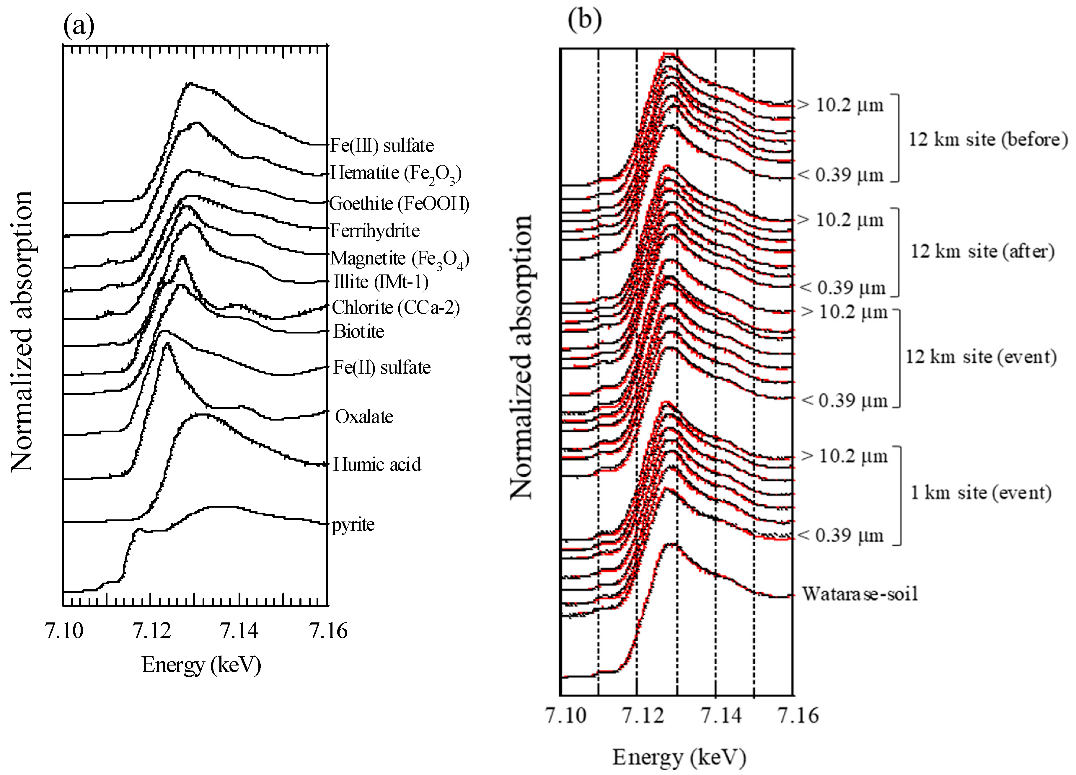
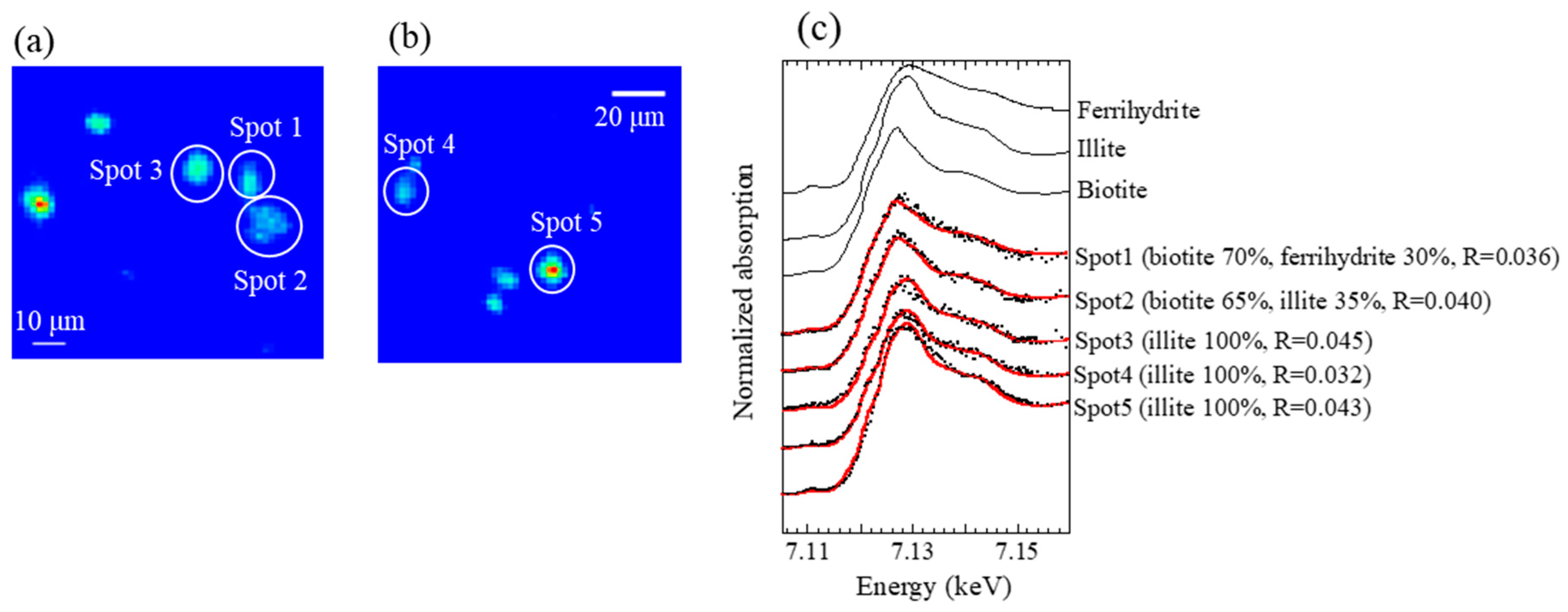
All XAFS spectra measured for aerosol samples were well fitted with (hydr)oxides (mainly ferrihydrite) and Fe-containing silicate minerals (mainly biotite and illite) (Figure A2 and Figure A3). Moreover, the presence of biotite, illite, and ferrihydrite were also confirmed via μ-XRF-XAFS analysis (Figure A4). The presence of these species were observed from Watarase soil (Figure A2 and Figure A3) and aerosols collected in Tsukuba and Hiroshima, Japan [7,18,62]. Before and after the event, ratios of silicate minerals (biotite and illite) were slightly higher in coarse particles than in fine particles, whereas the ratios of (hydr)oxides were higher in fine particles than in coarse particles. Iron (hydr)oxides, including ferrihydrite, are present in soils, whereas many reports have shown that nanoparticles of Fe (hydr)oxides are emitted by anthropogenic combustion [11]. Thus, these results suggested that anthropogenic Fe was also present in fine particles. During the event, ratios of silicate minerals in fine particles were slightly higher compared with those before and after the event. We compared the first derivatives of the spectra of the four sample sets at stage 6 (0.39–0.69 μm) because first derivatives can clarify slight spectral difference (Figure A4). The peaks of samples during the event had an obvious shoulder at 7.12 keV compared with those at the 12 km site before and after the event, which was possibly due to the influence of biotite and illite having different peak positions from that of ferrihydrite (Figure A4b). These results indicated that increased amounts of biotite/illite were present in the fine particles during the event, possibly due to the increased contribution of Fe in soil suspended by the burning event.
Figure A2.
Fe K-edge XANES spectra of (a) reference materials and (b) aerosol and soil samples. Black and red lines are raw spectra and fitting results, respectively.
Figure A2.
Fe K-edge XANES spectra of (a) reference materials and (b) aerosol and soil samples. Black and red lines are raw spectra and fitting results, respectively.

Figure A3.
Fraction of each Fe species of (a) the 12 km site before the event, (b) the 12 km site after the event, (c) the 12 km site during the event, (d) the 1 km site during the event, and (e) Watarase soil obtained from linear combination fitting of XANES spectra.
Figure A3.
Fraction of each Fe species of (a) the 12 km site before the event, (b) the 12 km site after the event, (c) the 12 km site during the event, (d) the 1 km site during the event, and (e) Watarase soil obtained from linear combination fitting of XANES spectra.
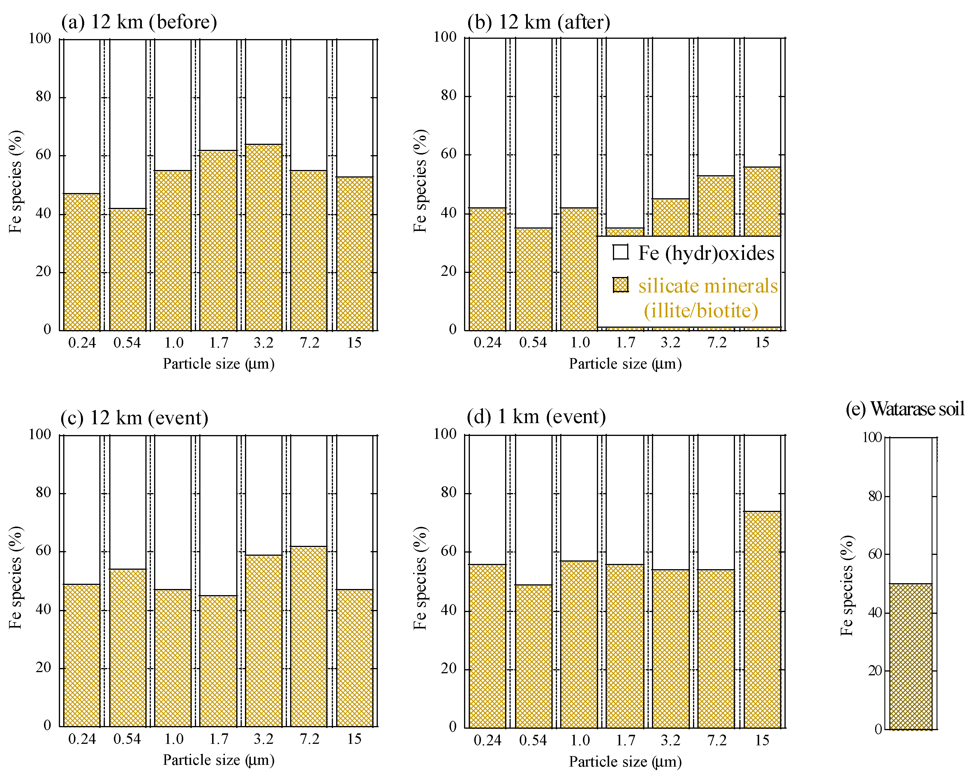
Figure A4.
(a) XANES spectra at stage 6; (b) first derivatives of the XANES spectra.

Figure A5.
(a,b) μ-XRF maps of Fe of coarse particles (stage 2; 4.9–10.2 μm) at the 1 km site during the event and (c) Fe K-edge XANES spectra of the spots in the maps.
Figure A5.
(a,b) μ-XRF maps of Fe of coarse particles (stage 2; 4.9–10.2 μm) at the 1 km site during the event and (c) Fe K-edge XANES spectra of the spots in the maps.

Appendix C
Figure A6.
Vapor pressures of FeCl3, FeCl2, and Fe at different temperatures calculated based on [59].
Figure A6.
Vapor pressures of FeCl3, FeCl2, and Fe at different temperatures calculated based on [59].

References
- Martin, J.H.; Fitzwater, S.E. Iron deficiency limits phytoplankton growth in the north-east Pacific subarctic. Nature 1988, 331, 341–343. [Google Scholar] [CrossRef]
- Martin, J.H.; Coale, K.H.; Johnson, K.S.; Fitzwater, S.E.; Gordon, R.M.; Tanner, S.J.; Hunter, C.N.; Elrod, V.A.; Nowicki, J.L.; Coley, T.L.; et al. Testing the iron hypothesis in ecosystems of the equatorial Pacific Ocean. Nature 1994, 371, 123–129. [Google Scholar] [CrossRef]
- Boyd, P.W.; Jickells, T.; Law, C.S.; Blain, S.; Boyle, E.A.; Buesseler, K.O.; Coale, K.H.; Cullen, J.J.; de Baar, H.J.W.; Follows, M.; et al. Mesoscale iron enrichment experiments 1993–2005: Synthesis and future directions. Science 2007, 315, 612–617. [Google Scholar] [CrossRef] [PubMed]
- Moore, C.M.; Mills, M.M.; Arrigo, K.R.; Berman-Frank, I.; Bopp, L.; Boyd, P.W.; Galbraith, E.D.; Geider, R.J.; Guieu, C.; Jaccard, S.L.; et al. Processes and patterns of oceanic nutrient limitation. Nat. Geosci. 2013, 6, 701–710. [Google Scholar] [CrossRef]
- Conway, T.M.; John, S.G. Quantification of dissolved iron sources to the North Atlantic Ocean. Nature 2014, 511, 212–215. [Google Scholar] [CrossRef] [PubMed]
- Sedwick, P.N.; Sholkovitz, E.R.; Church, T.M. Impact of anthropogenic combustion emissions on the fractional solubility of aerosol iron: Evidence from the Sargasso Sea. Geochem. Geophys. Geosyst. 2007, 8, 1–41. [Google Scholar] [CrossRef]
- Takahashi, Y.; Higashi, M.; Furukawa, T.; Mitsunobu, S. Change of iron species and iron solubility in Asian dust during the long-range transport from western China to Japan. Atmos. Chem. Phys. 2011, 11, 11237–11252. [Google Scholar] [CrossRef]
- Ito, A. Atmospheric processing of combustion aerosols as a source of bioavailable iron. Environ. Sci. Technol. Lett. 2015, 2, 70–75. [Google Scholar] [CrossRef]
- Schroth, A.W.; Crusius, J.; Sholkovitz, E.R.; Bostick, B.C. Iron solubility driven by speciation in dust sources to the ocean. Nat. Geosci. 2009, 2, 337–340. [Google Scholar] [CrossRef]
- Myriokefalitakis, S.; Ito, A.; Kanakidou, M.; Nenes, A.; Krol, M.C.; Mahowald, N.M.; Scanza, R.A.; Hamilton, D.S.; Johnson, M.S.; Meskhidze, N.; et al. Reviews and syntheses: The GESAMP atmospheric iron deposition model intercomparison study. Biogeosciences 2018, 15, 6659–6684. [Google Scholar] [CrossRef]
- Sanderson, P.; Delgado-Saborit, J.M.; Harrison, R.M. A review of chemical and physical characterisation of atmospheric metallic nanoparticles. Atmos. Environ. 2014, 94, 353–365. [Google Scholar] [CrossRef]
- Kopcewicz, B.; Kopcewicz, M.; Pietruczuk, A. The Mössbauer study of atmospheric iron-containing aerosol in the coarse and PM2.5 fractions measured in rural site. Chemosphere 2015, 131, 9–16. [Google Scholar] [CrossRef] [PubMed]
- Moteki, N.; Adachi, K.; Ohata, S.; Yoshida, A.; Harigaya, T.; Koike, M.; Kondo, Y. Anthropogenic iron oxide aerosols enhance atmospheric heating. Nat. Commun. 2017, 8, 1–11. [Google Scholar] [CrossRef] [PubMed]
- Uematsu, M.; Yoshikawa, A.; Muraki, H.; Arao, K.; Uno, I. Transport of mineral and anthropogenic aerosols during a Kosa event over East Asia. J. Geophys. Res. 2002, 107, 4059. [Google Scholar] [CrossRef]
- Maher, B.A.; Ahmed, I.A.M.; Karloukovski, V.; MacLaren, D.A.; Foulds, P.G.; Allsop, D.; Mann, D.M.A.; Torres-Jardón, R.; Calderon-Garciduenas, L. Magnetite pollution nanoparticles in the human brain. Proc. Natl. Acad. Sci. USA 2016, 113, 10797–10801. [Google Scholar] [CrossRef] [PubMed]
- Labatut, M.; Lacan, F.; Pradoux, C.; Chemeleff, J.; Radic, A.; Murray, J.W.; Poitrasson, F.; Johansen, A.M.; Thil, F. Iron sources and dissolved-particulate interactions in the seawater of the Western Equatorial Pacific, iron isotope perspectives. Glob. Biogeochem. Cycles 2014, 28, 1044–1065. [Google Scholar] [CrossRef]
- Kurisu, M.; Sakata, K.; Miyamoto, C.; Takaku, Y.; Iizuka, T.; Takahashi, Y. Variation of iron isotope ratios in anthropogenic materials emitted through combustion processes. Chem. Lett. 2016, 45, 970–972. [Google Scholar] [CrossRef]
- Kurisu, M.; Takahashi, Y.; Iizuka, T.; Uematsu, M. Very low isotope ratio of iron in fine aerosols related to its contribution to the surface ocean. J. Geophys. Res. Atmos. 2016, 121, 11119–11136. [Google Scholar] [CrossRef]
- Kurisu, M.; Adachi, K.; Sakata, K.; Takahashi, Y. Stable isotope ratios of combustion iron produced by evaporation in a steel plant. ACS Earth Space Chem. under review. [CrossRef]
- Beard, B.L.; Johnson, C.M.; Skulan, J.L.; Nealson, K.H.; Cox, L.; Sun, H. Application of Fe isotopes to tracing the geochemical and biological cycling of Fe. Chem. Geol. 2003, 195, 87–117. [Google Scholar] [CrossRef]
- Beard, B.L.; Johnson, C.M.; Von Damm, K.L.; Poulson, R.L. Iron isotope constraints on Fe cycling and mass balance in oxygenated Earth oceans. Geology 2003, 31, 629–632. [Google Scholar] [CrossRef]
- Guieu, C.; Bonnet, S.; Wagener, T.; Loÿe-Pilot, M.D. Biomass burning as a source of dissolved iron to the open ocean? Geophys. Res. Lett. 2005, 32, 1–5. [Google Scholar] [CrossRef]
- Paris, R.; Desboeufs, K.V.; Formenti, P.; Nava, S.; Chou, C. Chemical characterisation of iron in dust and biomass burning aerosols during AMMA-SOP0/DABEX: Implication for iron solubility. Atmos. Chem. Phys. 2010, 10, 4273–4282. [Google Scholar] [CrossRef]
- Winton, V.H.L.; Edwards, R.; Bowie, A.R.; Keywood, M.; Williams, A.G.; Chambers, S.D.; Selleck, P.W.; Desservettaz, M.; Mallet, M.D.; Paton-Walsh, C. Dry season aerosol iron solubility in tropical northern Australia. Atmos. Chem. Phys. 2016, 16, 12829–12848. [Google Scholar] [CrossRef]
- Dauphas, N.; Janney, P.E.; Mendybaev, R.A.; Wadhwa, M.; Richter, F.M.; Davis, A.M.; Van Zuilen, M.; Hines, R.; Foley, C.N. Hromatographic separation and multicollection-ICPMS analysis of iron. Investigating mass-dependent and -independent isotope effects. Anal. Chem. 2004, 76, 5855–5863. [Google Scholar] [CrossRef] [PubMed]
- Richter, F.; Dauphas, N.; Teng, F. Non-traditional fractionation of non-traditional isotopes: Evaporation, chemical diffusion and Soret diffusion. Chem. Geol. 2009, 258, 92–103. [Google Scholar] [CrossRef]
- Guelke, M.; Von Blanckenburg, F. Fractionation of stable iron isotopes in higher plants. Environ. Sci. Technol. 2007, 41, 1896–1901. [Google Scholar] [CrossRef] [PubMed]
- Mead, C.; Herckes, P.; Majestic, B.J.; Anbar, A.D. Source apportionment of aerosol iron in the marine environment using iron isotope analysis. Geophys. Res. Lett. 2013, 40, 5722–5727. [Google Scholar] [CrossRef]
- Streets, D.G.; Yarber, K.F.; Woo, J.-H.; Carmichael, G.R. Biomass burning in Asia: Annual and seasonal estimates and atmospheric emissions. Glob. Biogeochem. Cycles 2003, 17, 1–20. [Google Scholar] [CrossRef]
- Chen, J.; Li, C.; Ristovski, Z.; Milic, A.; Gu, Y.; Islam, M.S.; Wang, S.; Hao, J.; Zhang, H.; He, C.; Guo, H.; et al. A review of biomass burning: Emissions and impacts on air quality, health and climate in China. Sci. Total Environ. 2017, 579, 1000–1034. [Google Scholar] [CrossRef] [PubMed]
- Japan Meteorological Agency. Available online: www.jma.go.jp/jp/yoho/ (accessed on 11 October 2017).
- Sakata, K.; Kurisu, M.; Tanimoto, H.; Sakaguchi, A.; Uematsu, M.; Miyamoto, C.; Takahashi, Y. Custom-made PTFE filters for ultra-clean size-fractionated aerosol sampling for trace metals. Mar. Chem. 2018, 206, 100–108. [Google Scholar] [CrossRef]
- Keene, W.C.; Pszenny, A.A.P.; Galloway, J.N.; Hawley, M.E. Sea-salt corrections and interpretation of constituent ratios in marine precipitation. J. Geophys. Res. 1986, 91, 6647. [Google Scholar] [CrossRef]
- Luo, C.; Mahowald, N.; Bond, T.; Chuang, P.Y.; Artaxo, P.; Siefert, R.; Chen, Y.; Schauer, J. Combustion iron distribution and deposition. Glob. Biogeochem. Cycles 2008, 22, 1–17. [Google Scholar] [CrossRef]
- Hsu, S.C.; Wong, G.T.F.; Gong, G.C.; Shiah, F.K.; Huang, Y.T.; Kao, S.J.; Tsai, F.; Candice Lung, S.C.; Lin, F.J.; Lin, I.I.; et al. Sources, solubility, and dry deposition of aerosol trace elements over the East China Sea. Mar. Chem. 2010, 120, 116–127. [Google Scholar] [CrossRef]
- Morton, P.L.; Landing, W.M.; Hsu, S.C.; Milne, A.; Aguilar-Islas, A.M.; Baker, A.R.; Bowie, A.R.; Buck, C.S.; Gao, Y.; Gichuki, S.; et al. Methods for the sampling and analysis of marine aerosols: Results from the 2008 GEOTRACES aerosol intercalibration experiment. Limnol. Oceanogr. Methods 2013, 11, 62–78. [Google Scholar] [CrossRef]
- Takeichi, Y.; Inami, N.; Suga, H.; Takahashi, Y.; Ono, K. Compact scanning transmission X-ray microscope at the photon factory. AIP Conf. Proc. 2016, 1696. [Google Scholar] [CrossRef]
- Keiluweit, M.; Nico, P.S.; Johnson, M.G. Dynamic molecular structure of plant biomass-derived black carbon (biochar). Environ. Sci. Technol. 2010, 44, 1247–1253. [Google Scholar] [CrossRef] [PubMed]
- Chen, C.P.; Cheng, C.H.; Huang, Y.H.; Chen, C.-T.; Lai, C.M.; Menyailo, O.V.; Fan, L.J.; Yang, Y.W. Converting leguminous green manure into biochar: Changes in chemical composition and C and N mineralization. Geoderma 2014, 232–234, 581–588. [Google Scholar] [CrossRef]
- Albarède, F.; Telouk, P.; Blichert-Toft, J.; Boyet, M.; Agranier, A.; Nelson, B. Precise and accurate isotopic measurements using multiple-collector ICPMS. Geochim. Cosmochim. Acta 2004, 68, 2725–2744. [Google Scholar] [CrossRef]
- Weyer, S.; Anbar, A.D.; Brey, G.P.; Münker, C.; Mezger, K.; Woodland, A.B. Iron isotope fractionation during planetary differentiation. Earth Planet. Sci. Lett. 2005, 240, 251–264. [Google Scholar] [CrossRef]
- Atmospheric Environmental Information System. Available online: http://atmospheric-monitoring.jp/pref/tochigi/index.html (accessed on 1 February 2019).
- Andreae, M.O.; Browell, E.V.; Garstang, G.L.; Harriss, R.C.; Hill, G.F.; Jacobs, D.J.; Pereira, M.C.; Sachse, G.W.; Setzer, A.W.; Silva Dias, P.L.; et al. Biomass-burning emissions and associated haze layers over Amazonia. J. Geophys. Res. 1988, 93, 1509–1527. [Google Scholar] [CrossRef]
- Deng, C.; Zhuang, G.; Huang, K.; Li, J.; Zhang, R.; Wang, Q.; Liu, T.; Sun, Y.; Guo, Z.; Fu, J.S.; et al. Chemical characterization of aerosols at the summit of Mountain Tai in Central East China. Atmos. Chem. Phys. 2011, 11, 7319–7332. [Google Scholar] [CrossRef]
- Lamarque, J.F.; Bond, T.C.; Eyring, V.; Granier, C.; Heil, A.; Klimont, Z.; Lee, D.; Liousse, C.; Mieville, A.; Owen, B.; et al. Historical (1850-2000) gridded anthropogenic and biomass burning emissions of reactive gases and aerosols: Methodology and application. Atmos. Chem. Phys. 2010, 10, 7017–7039. [Google Scholar] [CrossRef]
- Echalar, F.; Gaudichet, A.; Cachier, H.; Artaxo, P. Aerosol emissions by tropical forest and savanna biomass burning: characteristic trace elements and fluxes. Geophys. Res. Lett. 1995, 22, 3039–3042. [Google Scholar] [CrossRef]
- Nriagu, J.O.; Pacnya, J.M. Quantative assessment of worldwide contamination of air, water and soils by trace metals. Nature 1988, 333, 134–139. [Google Scholar] [CrossRef] [PubMed]
- Artaxo, P.; Storms, H.; Bruynseels, F.; Van Grieken, R.; Maenhaut, W. Composition and sources of aerosols from the Amazon Basin. J. Geophys. Res. 1988, 93, 1605–1615. [Google Scholar] [CrossRef]
- Yamada, E.; Funoki, S.; Abe, Y.; Umemura, S.; Yamaguchi, D.; Fuse, Y. Size distribution and characteristics of chemical components in ambient particulate matter. Anal. Sci. 2005, 21, 89–94. [Google Scholar] [CrossRef] [PubMed]
- Cuiping, L.; Chuangzhi, W.; Yanyongjie; Haitao, H. Chemical elemental characteristics of biomass fuels in China. Biomass Bioenergy 2004, 27, 119–130. [Google Scholar] [CrossRef]
- Barker, A.V.; Pilbeam, D.J. Handbook of Plant Nutrition; CRC press: Boca Raton, FL, USA, 2007. [Google Scholar]
- Taylor, S.R. Abundance of chemical elements in the continental crust: A new table. Geochim. Cosmochim. Acta 1964, 28, 1273–1285. [Google Scholar] [CrossRef]
- Andreae, M.O. Soot carbon and excess fire potassium: Long-range transport of combustion-derived aerosols. Science (80-.) 1983, 220, 1148–1151. [Google Scholar] [CrossRef] [PubMed]
- Mahowald, N.M.; Hamilton, D.S.; Mackey, K.R.M.; Moore, J.K.; Baker, A.R.; Scanza, R.A.; Zhang, Y. Aerosol trace metal leaching and impacts on marine microorganisms. Nat. Commun. 2018, 9, 1–15. [Google Scholar] [CrossRef] [PubMed]
- Andreae, M.O.; Artaxo, P.; Fischer, H.; Freitas, S.R.; Gregoire, J.-M.; Hansel, A.; Hoor, P.; Kormann, R.; Krejci, R.; Lange, L.; et al. Transport of biomass burning smoke to the upper troposphere by deep convection in the equatorial region. Geophys. Res. Lett. 2001, 28, 951–954. [Google Scholar] [CrossRef]
- Artaxo, P.; Martins, J.V.; Yamasoe, M.A.; Procópio, A.S.; Pauliquevis, T.M.; Andreae, M.O.; Guyon, P.; Gatti, L.V.; Leal, A.M.C. Physical and chemical properties of aerosols in the wet and dry seasons in Rondônia, Amazonia. J. Geophys. Res. D Atmos. 2002, 107, 1–14. [Google Scholar] [CrossRef]
- Siefert, R.L.; Webb, S.M.; Hoffmann, M.R. Determination of photochemically available iron in ambient aerosols. J. Geophys. Res. 1996, 101, 14441–14449. [Google Scholar] [CrossRef]
- Miller, A.; Ahlstrand, G.; Kittelson, D.; Zachariah, M. The fate of metal (Fe) during diesel combustion: Morphology, chemistry, and formation pathways of nanoparticles. Combust. Flame 2007, 149, 129–143. [Google Scholar] [CrossRef]
- Kubaschewski, O.; Alcock, C.B. Metallurgical Thermochemistry, 3rd ed.; Pergamon: Oxford, UK, 1979. [Google Scholar]
- Symonds, R.B.; Reed, M.H.; Rose, W.I. Origin, speciation, and fluxes of trace-element gases at Augustine volcano, Alaska: Insights into magma degassing and fumarolic processes. Geochim. Cosmochim. Acta 1992, 56, 633–657. [Google Scholar] [CrossRef]
- Stein, A.F.; Draxler, R.R.; Rolph, G.D.; Stunder, B.J.B.; Cohen, M.D.; Ngan, F. Noaa’s hysplit atmospheric transport and dispersion modeling system. Bull. Am. Meteorol. Soc. 2015, 96, 2059–2077. [Google Scholar] [CrossRef]
- Takahashi, Y.; Furukawa, T.; Kanai, Y.; Uematsu, M.; Zheng, G.; Marcus, M.A. Seasonal changes in Fe species and soluble Fe concentration in the atmosphere in the Northwest Pacific region based on the analysis of aerosols collected in Tsukuba, Japan. Atmos. Chem. Phys. 2013, 13, 7695–7710. [Google Scholar] [CrossRef]
Figure 1.
(a) Large scale map of the sampling area. The map was made by General Mapping Tools map generator (http://woodshole.er.usgs.gov/mapit/). The sampling points are plotted in detailed map (b) obtained from Geospatial Information Authority of Japan (https://maps.gsi.go.jp/development/ichiran.html).

Figure 2.
Concentrations of PM2.5 during the sampling periods observed at the 12 km site (Oyama City Office) obtained from Atmospheric Environmental Information System (http://atmospheric-monitoring.jp/pref/tochigi/index.html).
Figure 2.
Concentrations of PM2.5 during the sampling periods observed at the 12 km site (Oyama City Office) obtained from Atmospheric Environmental Information System (http://atmospheric-monitoring.jp/pref/tochigi/index.html).
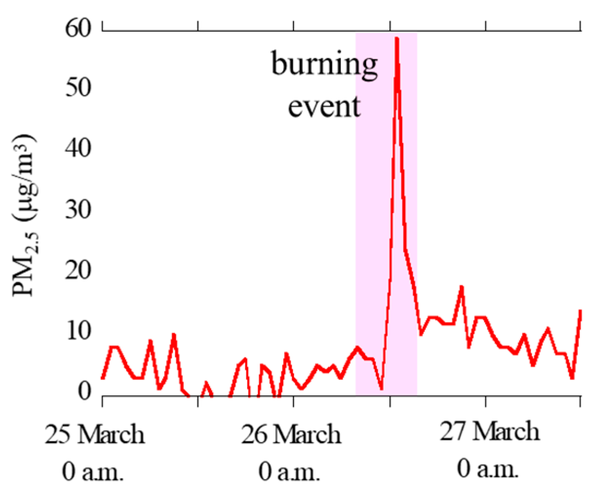
Figure 3.
Size distributions of concentrations of (a) Cl−, (b) NO3−, (c) C2O4, (d) SO42−, (e) Na+, (f) NH4+, (g) K+, (h) Mg2+, (i) Ca2+, (j) nss-K+, and (k) nss-SO42− in aerosols. Averaged values of the event (the 1 km and 12 km site samples during the event) and the non-event (the 12 km site samples before and after the event) were shown. Errors are standard deviation of the two values.
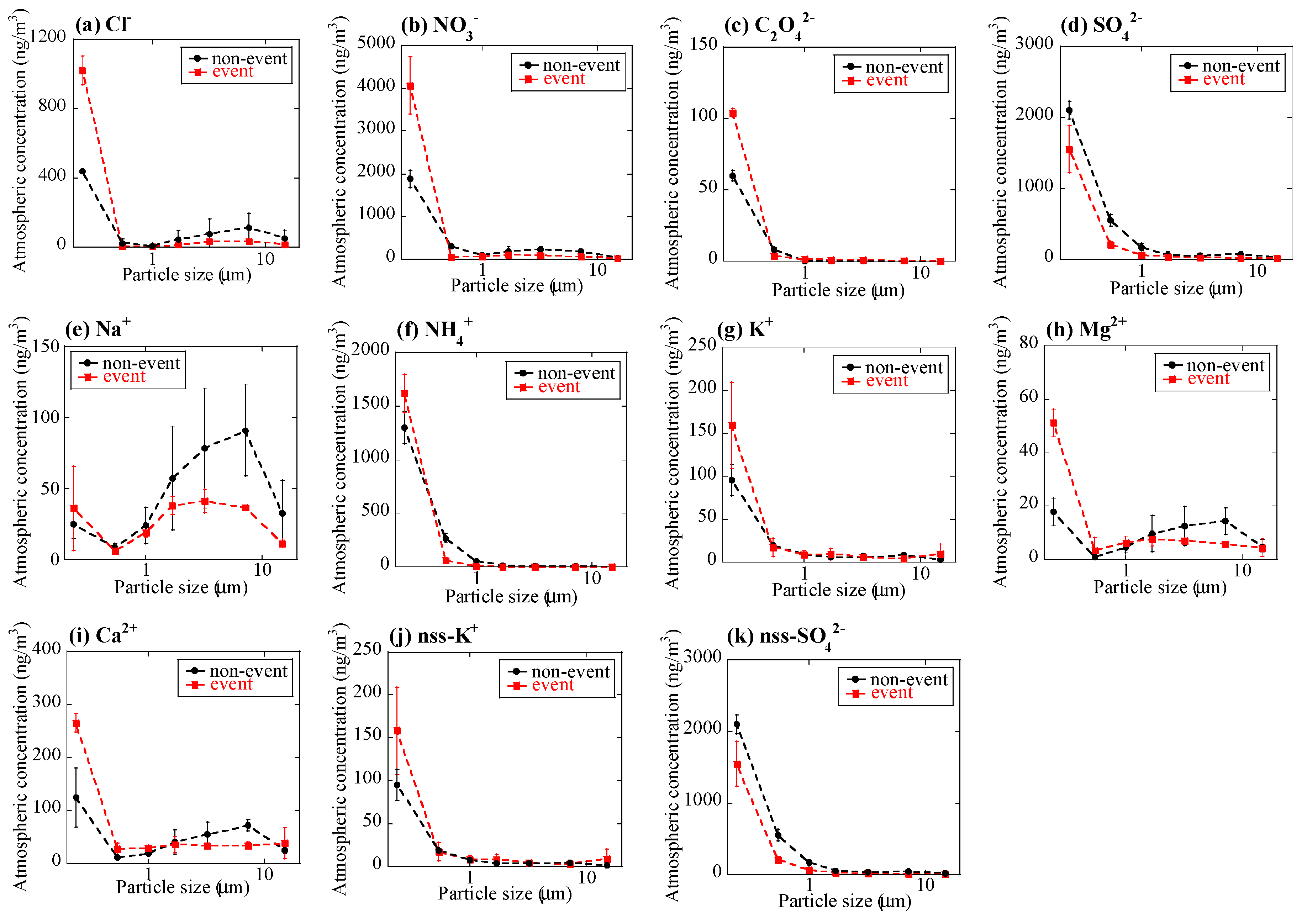
Figure 4.
Size distributions of concentrations of (a) Al, (b) Ti, (c) Fe, (d) Zn, and (e) Pb of aerosols. Averaged values of the event (the 1 km and 12 km site samples during the event) and the non-event (the 12 km site samples before and after the event) were shown. Errors are standard deviation of the two values.

Figure 5.
Enrichment factors of (a) Ti, (b) Fe, (c) Zn, and (d) Pb of size-fractionated aerosols defined as (M/Al)sample/(M/Al)watarase-soil (M is target elements). Averaged values of the event (the 1 km and 12 km site samples during the event) and the non-event (the 12 km site samples before and after the event) were shown. Errors are standard deviation of the two values.

Figure 6.
Enrichment factors of Ti, Fe, and nss-K+ during the event. Soluble K in soil was 0.080 wt %, which was used for the calculation.
Figure 6.
Enrichment factors of Ti, Fe, and nss-K+ during the event. Soluble K in soil was 0.080 wt %, which was used for the calculation.

Figure 7.
Fractional Fe solubility of size-fractionated aerosols extracted by ultrapure water.
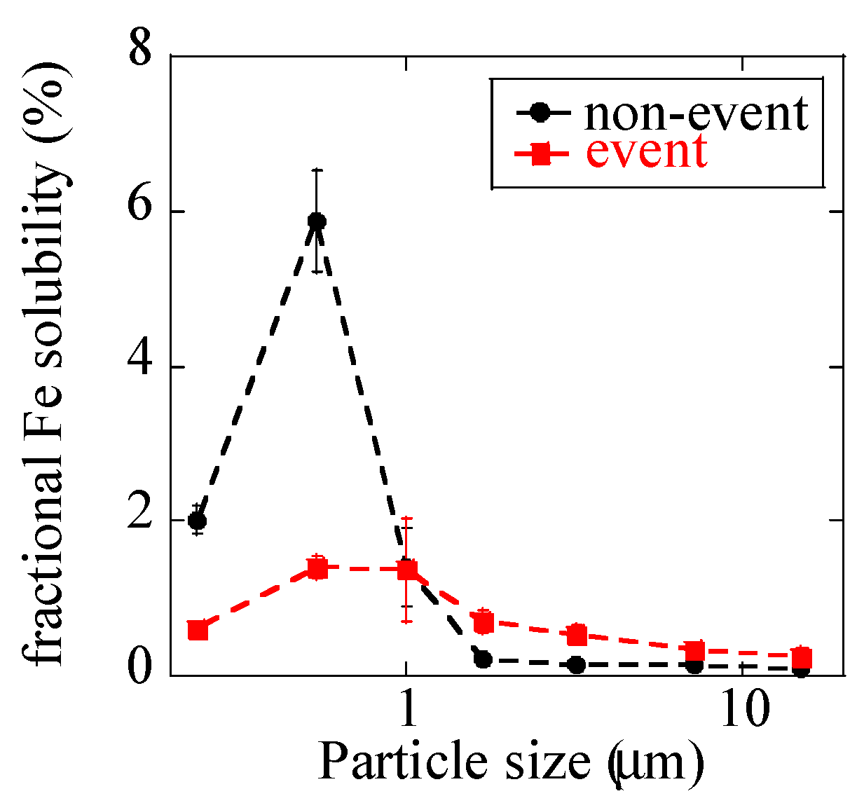
Figure 8.
(a) C K-edge spectra of several particles collected at 1 km site during the event. Energy step numbers were limited except for the bottom spectra to avoid beam damage. (b) C K-edge spectra of grass heated at temperatures 100–700 °C. The figure was reprinted with permission from reference [38]. Copyright (2010), American Chemical Society.
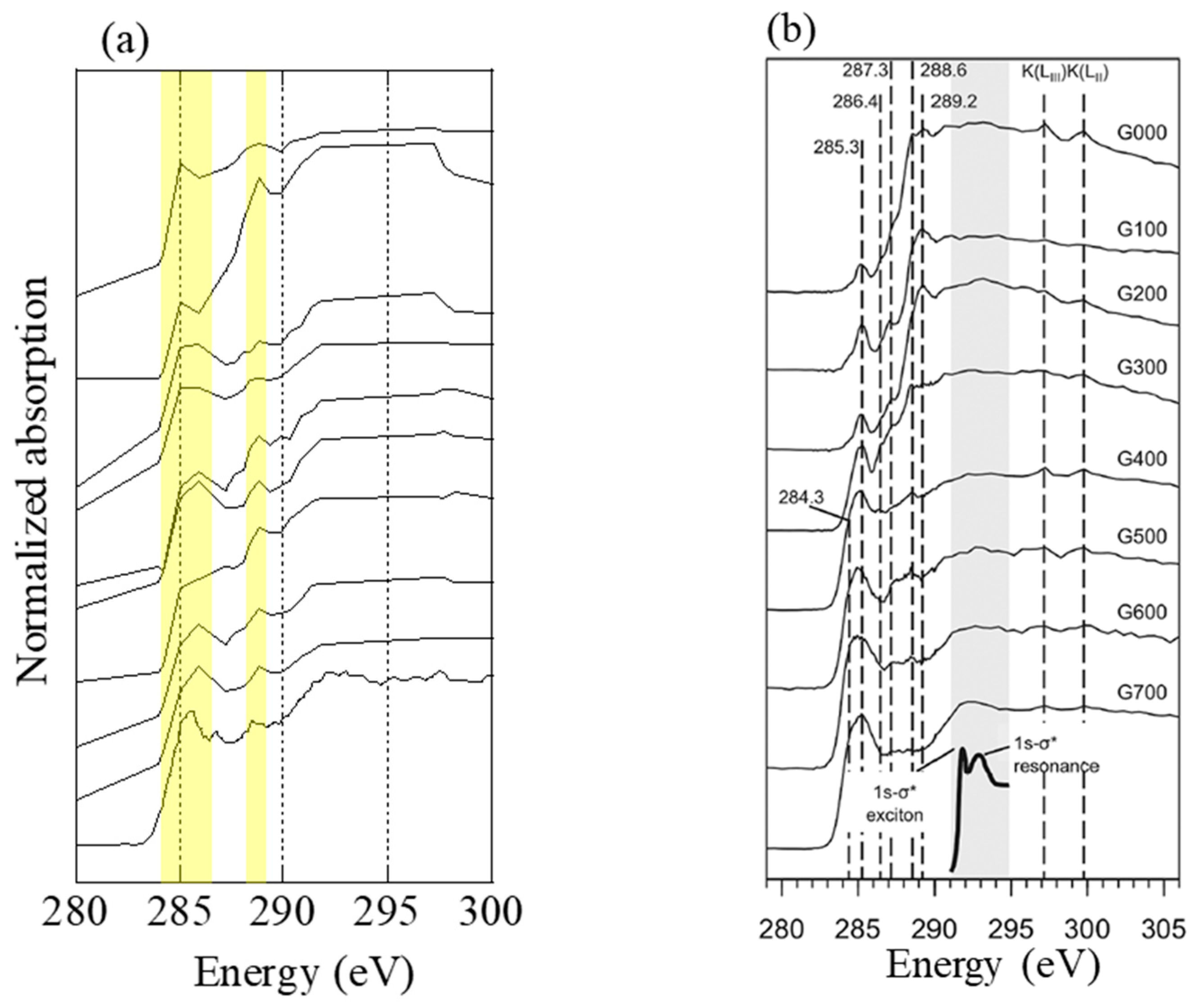
Figure 9.
Size distributions of δ56Fe values of the aerosols collected near Watarase Basin.
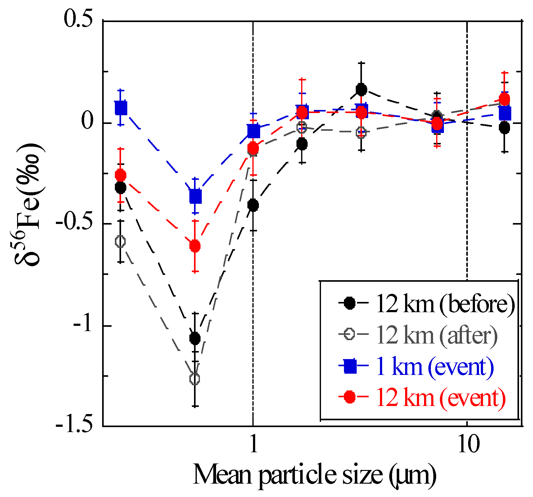
Figure 10.
δ56Fe values of total (acid-digested) and soluble Fe at stage 6 (0.39–0.69 μm). Soluble Fe fractions are shown next to the plots.
Figure 10.
δ56Fe values of total (acid-digested) and soluble Fe at stage 6 (0.39–0.69 μm). Soluble Fe fractions are shown next to the plots.

Figure 11.
(a) Size distributions of δ56Fe values of the size-fractionated aerosol particles collected in a tunnel [17] and near Watarase Basin in this study; Correlation of δ56Fe values and inverse of Fe concentrations of size-fractionated particles collected (b) in the tunnel and (c) near Watarase Basin.

Table 1.
Aerosol sampling periods (in local time) at the 12 km site (Oyama City Office) and the 1 km site (Shimonamai Elementary School)
Table 1.
Aerosol sampling periods (in local time) at the 12 km site (Oyama City Office) and the 1 km site (Shimonamai Elementary School)
| Sample | Start | End | Total Flow Volume (m3) |
|---|---|---|---|
| 12 km (before) | 19 March 2016, 12:22 p.m. | 26 March 2016, 6:47 a.m. | 5265.3 |
| 12 km (event) | 26 March 2016, 7:07 a.m. | 26 March 2016, 6:15 p.m. | 385.6 |
| 1 km (event) | 26 March 2016, 7:59 a.m. | 26 March 2016, 4:55 p.m. | 300.4 |
| 12 km (after) | 26 March 2016, 6:34 a.m. | 31 March 2016 1:42 p.m. | 3996.8 |
Table 2.
Concentrations of Al, TI, Fe, Zn, and Pb of Watarase soil, reed at Watarase Basin, and various plants
Table 2.
Concentrations of Al, TI, Fe, Zn, and Pb of Watarase soil, reed at Watarase Basin, and various plants
| Element | Watarase Soil (wt %) | Reed (wt %, Dry Biomass Basis) | Various Plants [50,51] (wt %, Dry Biomass Basis) |
|---|---|---|---|
| K | 0.64 | 0.26 | 0.1–7 |
| Al | 4.2 | 0.016 | 0.001–0.5 |
| Ti | 0.20 | 0.00083 | 0.001–0.02 |
| Fe | 2.2 | 0.013 | 0.002–0.5 |
| Zn | 0.04 | 0.00097 | 0.001–0.02 |
| Pb | 0.002 | 0.00025 | 0.00001–0.006 |
© 2019 by the authors. Licensee MDPI, Basel, Switzerland. This article is an open access article distributed under the terms and conditions of the Creative Commons Attribution (CC BY) license (http://creativecommons.org/licenses/by/4.0/).
Share and Cite
MDPI and ACS Style
Kurisu, M.; Takahashi, Y. Testing Iron Stable Isotope Ratios as a Signature of Biomass Burning. Atmosphere 2019, 10, 76. https://doi.org/10.3390/atmos10020076
AMA Style
Kurisu M, Takahashi Y. Testing Iron Stable Isotope Ratios as a Signature of Biomass Burning. Atmosphere. 2019; 10(2):76. https://doi.org/10.3390/atmos10020076
Chicago/Turabian StyleKurisu, Minako, and Yoshio Takahashi. 2019. "Testing Iron Stable Isotope Ratios as a Signature of Biomass Burning" Atmosphere 10, no. 2: 76. https://doi.org/10.3390/atmos10020076
Note that from the first issue of 2016, this journal uses article numbers instead of page numbers. See further details here.