Machine Learning-Based Spectral Library for Crop Classification and Status Monitoring

Abstract

The establishment and application of a spectral library is a critical step in the standardization and automation of remote sensing interpretation and mapping. Currently, most spectral libraries are designed to support the classification of land cover types, whereas few are dedicated to agricultural remote sensing monitoring. Here, we gathered spectral observation data on plants in multiple experimental scenarios into a spectral database to investigate methods for crop classification (16 crop species) and status monitoring (tea plant and rice growth). We proposed a set of screening methods for spectral features related to plant classification and status monitoring (band reflectance, vegetation index, spectral differentiation, spectral continuum characteristics) that are based on ISODATA and JM distance. Next, we investigated the performance of different machine learning classifiers in the spectral library application, including K-nearest neighbor (KNN), Random Forest (RF), and a genetic algorithm coupled with a support vector machine (GA-SVM). The optimal combination of spectral features and the classifier with the highest classification accuracy were selected for crop classification and status monitoring scenarios. The GA-SVM classifier performed the best, which produced an accuracy of OAA = 0.94, Kappa = 0.93 for crop classification in a complex scenario (crops mixed with 71 non-crop plant species), and promising accuracies for tea plant growth monitoring (OAA = 0.98, Kappa = 0.97) and rice growth stage monitoring (OAA = 0.92, Kappa = 0.90). Therefore, the establishment of a plant spectral library combined with relevant feature extraction and a classification algorithm effectively supports agricultural monitoring by remote sensing.

1. Introduction

Agricultural remote sensing technology plays an important role in agricultural macromanagement, providing an efficient tool for monitoring agricultural field distribution [1] and crop growth [2], and for estimating of crop yields [3]. Hyperspectral remote sensing can obtain rich spectral information about plants and detect their physiological and biochemical status. Compared with multi-spectral remote sensing technology, hyperspectral remote sensing provides more detailed plant monitoring information, especially in complex scenarios [4] (e.g., mixed crop planting or mixed crop growth status). With the recent development and maturity of airborne and space-borne hyperspectral sensors, hyperspectral remote sensing is becoming an increasingly important technology with great potential for the remote monitoring of vegetation and agriculture [5].

Plant classification and growth status monitoring are useful applications of remote sensing technology and much progress has been made in combining hyperspectral technology and machine learning methods in recent years.

Table 1. Application of Machine Learning.

Monitoring Contents	Machine Learning Methods	Accuracy	Reference
Urban tree species (13 species)	Segmented canonical discriminant analysis (CDA), segmented principal component analysis (PCA), segmented stepwise discriminate analysis (SDA), and segmented maximum likelihood classifier (MLC)	OAA:76–96%	Pu and Liu [6]
Invasive species (Carpobrotus edulis, Cortaderia jubata, Eucalyptus globulus)	PCA and minimum noise fraction (MNF)	OAA:37–75%	Underwood et al. [7]
Nonnative plant species (Carpobrotus edulis, jubata grass, and Cortaderia jubata)	MLC	OAA:55–97%	Underwood et al. [8]
Juvenile tree species (9 species)	Maximum likelihood (ML)	OAA:68–96%	Huang et al. [9]
Soybean growth	Random forest (RF), artificial neural network (ANN), support vector machine (SVM)	R2:0.674–0.749	Yuan et al. [10]
Tobacco leaf nitrogen levels	SVM, supervised relevance neural gas (SRNG), generalized relevance learning vector quantization (GRLVQ), radial basis function (RBF)	OAA:2.2–99.8%	Backhaus et al. [11]
Wheat growth stages	iterative self-organizing data analysis (ISODATA), artificial immune system (AIS), hierarchical artificial immune system (HAIS), niche stratified artificial immune system (NHAIS)	OAA:59.5–81.5%	Senthilnath et al. [12]
Potato disease (Late Blight)	Multi-layer perceptron (MLP), convolutional neural network (CNN), support vector regression (SVR), random forest (RF)	R2:0.44–0.74	Duarte-Carvajalino [13]

shows some applications of machine learning. Pu and Liu [6] used hyperspectral data measured on the ground to identify 13 species of trees distributed in Tampa, Florida, USA, by segmented canonical discriminant analysis (CDA), segmented principal component analysis (PCA), segmented stepwise discriminate analysis (SDA), and segmented maximum likelihood classifier (MLC). With this method, the highest identification accuracy the authors achieved was 96%. Underwood et al. [7,8] used multiple minimum noise fraction (MNF) converted from AVIRIS hyperspectral image data to successfully classify three exotic plant species (iceplant, jubata grass, and blue gum) along the California coast based on MLC. Huang et al. [9] used UAV hyperspectral data and the maximum likelihood (ML) method to successfully identify saplings in wooded areas with a high accuracy of 95.7%. In terms of monitoring plant growth status, Yuan et al. [10] used UAV hyperspectral data to analyze soybean growth from leaf count estimates by combining random forest (RF), artificial neural network (ANN), and support vector machine (SVM) classifiers. The approach achieved an identification accuracy of R² = 0.749 (R² is the validation coefficient of the regression model). Backhaus et al. [11] used hyperspectral image data to monitor nitrogen levels in tobacco leaves, combining the classification methods of SVM, supervised relevance neural gas (SRNG), generalized relevance learning vector quantization (GRLVQ), and radial basis function (RBF), and achieved 99.8% accuracy in the classification of nutritional status. Senthilnath et al. [12] used satellite hyperspectral image data and the iterative self-organizing data analysis (ISODATA), the artificial immune system (AIS), the hierarchical artificial immune system (HAIS), and the niche stratified artificial immune system (NHAIS) classification method to successfully identify three growth stages of wheat crops and monitor growth, achieving an 81.5% identification accuracy. Duarte-Carvajalino [13] monitored potato late blight using UAV hyperspectral data and color images combined with the multi-layer perceptron (MLP), the support vector regression (SVR), the random forest (RF), and the convolutional neural network (CNN) classifiers, achieving a disease identification accuracy of R² = 0.74.

A critical step in the standardization and automation of remote sensing monitoring of plants is the establishment of a plant spectral library. Some spectral libraries have been created and applied, including spectral collections by NASA’s Jet Propulsion Laboratory (JPL), Johns Hopkins University (JHU), and the United States Geological Survey (USGS), which include spectra from rocks, minerals, lunar soils, terrestrial soils, manmade materials, meteorites, vegetation, snow, and ice [14]. However, most spectral libraries were designed to support comprehensive classification of land cover types rather than for agricultural remote sensing monitoring. Nidamanuri et al. [15] used HyMAP airborne hyperspectral images to establish a spectral library containing five crops (alfalfa, winter barley, winter rape, winter rye, and winter wheat) and achieved a crop classification accuracy of 82% by searching and matching the spectral library. This demonstrates that the joint hyperspectral remote sensing data and spectral library approach can be used to successfully monitor crops remotely. However, little research has been conducted on the construction and application of spectral libraries designed specifically for crop monitoring. In addition, spectral library-related techniques have largely been used for plant classification rather than for plant status monitoring, which is essential in agricultural production management. In this study, to promote the development of spectral library-based agricultural monitoring, the specific objectives were to: (1) obtain spectral data sets for crop classification in complex scenarios (crops mixed with non-crop plant species) and spectral data for crop status monitoring (i.e., growth vigor of tea plant and growth stages of rice) and used the tea plant data to construct a crop spectral library; (2) presented a set of spectral feature optimization methods and classification modeling methods for crop classification and status monitoring; (3) evaluated the effectiveness of the spectral library-based methods in crop classification and status monitoring.

2. Materials and Methods

2.1. Data Acquisition for Construction of a Crop Spectral Library

2.1.1. Experiment 1: Spectral Data Collection for Crop Classification

In this study, 16 major crops were selected for canopy spectral collection in the range of longitude 119.94°–120.35° and latitude 30.08°–30.32° in Hangzhou, Zhejiang province, from May to September 2017. Crops are often mixed with non-crop plants (e.g., urban garden and wetland plants) in the same landscape, so crop classification based on satellite or UAV remote sensing images under natural circumstances would include these non-crop plants. Therefore, in this study, we selected 71 non-crop plants commonly found in the study area for spectral collection. In terms of plant species investigation, some spectral collection points contained clear classification information on plant tags and could be used directly. When no listing information was available, species information was determined by an experienced plant ecologist according to the book of “Flora of China.” During the plant survey, each plant species was photographed for reference. The specific information collected on the 87 plant species (crops + non-crop plants) is shown in

Table A1. Plant species information. (ID 1–16 are crops; ID 17–87 are non-crop plants).

ID	Plant Common Name	Species Name	ID	Plant Common Name	Species Name
1	Citrus	Citrus reticulata Blanco	45	Phaseolus Vulgaris	Radermachera sinica (Hance) Hemsl.
2	Peach	Amygdalus persica Linn.	46	Larix Principis-Rupprechtii	Larix gmelinii var. principis-rupprechtii (Mayr) Pilg.
3	Ginkgo	Ginkgo biloba L.	47	Banana	Musa basjoo Siebold
4	Loquat	Eriobotrya japonica (Thunb.) Lindl.	48	Calycanthaceae	Calycanthaecae
5	Shaddock	Citrus maxima (Burm.) Osbeck	49	Podocarpus	Podocarpus macrophyllus D. Don
6	Cowpea	Vigna unguiculate (Linn.) Walp.	50	Bougainvillea	Bougainvillea spectabilis Willd.
7	Soybean	Glycine max (L.) Merr.	51	Japanese Five-Needle Pine	Pinus parviflora Sieb. et Zucc.
8	Sweet Potato	Ipomoea batatas (L.) Poir.	52	Evergreen	Rohdea japonica (Thunb.) Roth
9	Peanut	Arachis hypogaea Linn.	53	Platycladus Orientalis	Platycladus orientalis (Linn.) Franco
10	Amaranth	Amaranthus tricolor Linn.	54	Ligustrum Lucidum	Ligustrum lucidum Ait.
11	Eggplant	Solanum melongena Linn.	55	Phyllostachys Crenata	Bambusa multiplex’ Fernleaf’ R. A. Young
12	Sesame	Sesamum indicum Linn.	56	Cycas	Cycas revoluta Thunb
13	Youxian Camellia Oleifera	Camellia yuhsienensis Hu	57	Elm	Ulmus pumila L.
14	Rice	Oryza sativa	58	Pseudolarix	Pseudolarix amabilis (Nelson) Rehd.
15	Wheat	Triticum aestivum Linn.	59	Forsythia	Duranta erecta L.
16	Tea	Camellia sinensis (L.) O. Ktze.	60	Dragon Cypress	Juniperus chinensis’ Kaizuka’
17	Buxus Microphylla	Buxus sinica var. parvifolia M. Cheng	61	Sunflower	Helianthus annuus Linn.
18	Herb Trinity	Viola tricolor Linn.	62	Zelkova Schneideriana	Zelkova schneideriana Hand. -Mazz.
19	Elaeocarpus Decipiens	Elaeocarpus decipiens Hemsl.	63	Bambusa Multiplex	Bambusa multiplex ’Alphonso-Karrii’ R. A. Young
20	Handkerchief Tree	Davidia involucrate Baill.	64	Yulan Magnolia	Yulania denudate (Desr.) D. L. Fu
21	Camphor Tree	Cinnamomum camphora (L.) J.Presl.	65	Wisteria	Wisteria sinensis (Sims) Sweet
22	Michelia Maudiae	Michelia maudiae Dunn.	66	Rhus Succedanea	Toxicodendron succedaneum (Linn.) O. Kuntze
23	Chinese Pagoda Tree	Sophora japonica’ Pendula’ Hort.	67	Hibiscus Mutabilis	Hibiscus mutabilis Linn.
24	Plum Blossom	Armeniaca mume Sieb.	68	Awn	Miscanthus sinensis Anderss.
25	Red Wooden	Loropetalum chinense var. rubrum Yieh	69	Ilex Crenata	Ilex crenata Thunb.
26	Magnolia	Magnolia grandiflora L.	70	Willow	Salix babylonica Linn.
27	Japanese Maple	Acer palmatum Thunb.	71	Rudbeckia Laciniata	Rudbeckia laciniate Linn.
28	Cedar	Cedrus deodara (Roxb.) G. Don	72	Eleusine Indica	Eleusine indica (Linn.) Gaertn.
29	White Oak	Quercus fabri Hance	73	Soapberry	Sapindus Saponaria L.
30	Pampasgrass	Cortaderia selloana (Schult.) Aschers. et Graebn.	74	Reed Bamboo	Arundo donax L.
31	Red Maple	Acer palmatum’ Atropurpureum’	75	Banana Shrub	Michelia figo (Lour.) Spreng.
32	Sweet-Scented Osmanthus	Osmanthus fragrans Lour.	76	Sedum Sinensis	Sedum sarmentosum Bunge
33	Hackberry	Celtis sinensis Pers.	77	Rhododendron	Rhododendron simsii Planch.
34	Illicium Lanceolatum	Illicium lanceolatum A. C. Sm.	78	Lotus	Nelumbo nucifera Gaertn.
35	Bambusa Vulgaris Schrad	Phyllostachys aureosulcata’ Spectabilis’	79	Pyracantha	Pyracantha fortuneana (Maxim.) Li
36	Ilex Cornuta	Ilex cornuta Lindl. et Paxt.	80	Hasaki	Euonymus japonicus’ Aureo-marginatus’
37	Canna	Canna indica L.	81	Ligustrum Lucidum	Ligustrum vicaryi Rehder
38	Petunia Hybrida	Petunia hybrida Vilmorin	82	Paspalum	Paspalum thunbergii Kunth ex Steud.
39	Liquidambar Formosana	Liquidambar formosana Hance	83	Torenia Fournieri	Torenia fournieri Linden. ex Fourn.
40	Palm	Trachycarpus fortune (Hook.) H. Wendl.	84	Graperoot	Mahonia fortune (Lindl.) Fedde
41	Dalbergia	Dalbergia hupeana Hance	85	Moor Besom	Photinia serratifolia (Desf.) Kalkman
42	Camellia Puniceiflora Chang	Camellia puniceiflora H. T. Chang	86	Pink	Dianthus chinensis Linn.
43	Carbungi	Typha angustifolia L.	87	Marigold	Tagetes erecta Linn.
44	Phyllostachys Heterocycla	Phyllostachys edulis’ Heterocycla’

(Appendix A). The canopy spectral measurement for each species was repeated 25 times, providing a total of 2,175 pieces of original data were obtained. A small number of abnormal spectra were removed after data examination, for a final total of 2,147 spectra.

2.1.2. Experiment 2: Spectral Data Collection for Crop Growth Monitoring

Crop growth monitoring included two experiments: (1) growth status of tea plants and (2) growth stages of rice. We obtained canopy spectra and ancillary information for different crop statuses. Specific experimental information is shown in

Table 2. Crop growth status monitoring information in Experiment 2.

Plants’ Name	Status	Time	Location	Sample Size
Tea tree	Growth (Three levels)	August 2017	Hangzhou, China tea laboratory base	14 × 10 (poor growth) + 16 × 10 (medium growth) + 16 × 10 (good growth) = 460
Rice	Growing stage (Five stages)	August 2018	Fu yang, Hangzhou, China National Rice Research Institute	5 (stages) × 12 (plots) × 5 = 300

.

Experiment on Tea Plant Growth Vigor Monitoring

The tea plant growth monitoring experiment was conducted in August 2017 at the experimental base of Tea Research Institute, Chinese Academy of Agricultural Sciences in Hangzhou. The experimental base contains a total of 46 experimental plots (14 experimental plots applied less nutrition, 16 experimental plots applied the recommended rate of nutrition and 16 experimental plots applied over the recommended rate of nutrition) in which we obtained different levels of tea plant growth vigor by controlling nutrient inputs. In addition to collecting spectral data for each plot (10 times measurements in each plot), we also investigated tea plants growth vigor in the field. Vigor was evaluated by experienced cultivation experts from the China Tea Institute based on the following criteria: (1) good growth: lush leaf growth with 100% coverage, bright green leaf color, and normal plant height; (2) medium growth: sparse leaves, partial gaps in the canopy, dark green leaf color, and relatively low plant height; (3) poor growth: sparse leaves, crown gap, gray leaf color, relatively low plant height, and partial water loss and wilting in some leaves. Figure 1 demonstrated tea plants from the experimental area under different growth vigor.

Experiment on Rice Growth Stage Monitoring

The experiment was conducted in August 2018 at the experimental base of China National Rice Research Institute (CNRRI) for monitoring rice growth stages. Rice seedlings were transplanted into the experimental field on five different dates (1 week apart in sequence). Grade 5 was the latest sowing date and grade 1 was the earliest. Each treatment contained 12 plots and each plot area was 2 m × 4 m. Conventional management of fertilization and irrigation was applied in all treatments. In addition to collecting spectrometric data for each plot, rice growth stage was investigated by a rice cultivation expert from the CNRRI. Rice growth stage in each plot was observed during the elongation and booting stages.

2.1.3. Measurement of Crop Canopy Hyperspectral Data

Plant canopy spectra were measured using an ASD FieldSpec4 Pro FR (350–2500 nm) spectrometer in strict accordance with standard methods. The spectral resolution of the instrument is 3 nm in the 350–1000 nm range and 10 nm in the 1000–2500 nm range. During observation, the probe was pointed vertically downward at a height of 0.6 m above the ground and a field angle of 25°. In addition, each spectral reading is an average of 10 repeats of spectral records, which thus guaranteed the stability and high quality of the spectral data. Reflectance was obtained by calibration with a standard reference plate before and after each measurement. We used ViewSpec software and resampled the spectral curves to 1 nm. All spectroscopic measurements were made on clear, cloudless days between 10:00 and 14:00 (local time).

2.2. Extraction and Analysis of Spectral Features

2.2.1. Extraction of Spectral Features

Given the relatively large number of wavebands of spectral measurements (n = 2151) compared with directly using the spectral bands in classification, analysis efficiency can be enhanced by using fewer selected spectral features. Here we selected and extracted different types of spectral features for analysis according to the spectral characteristics of plants, including: (1) some original spectral bands; (2) a set of derivative and continuum-removal spectral features (Der & Con features) that can highlight the characteristics of peaks and valleys in spectral curves (

Table 3. Derivative and continuous removal spectral features used in this study.

Feature Type	Position	Band Range (nm)	Feature
First derivative feature	Blue edge	490–540	Maximum differential value (BMV)
			Position of the maximum differential value (BPMV)
			Sum of differential values (BSV)
	Yellow edge	540–620	Maximum differential value (YMV)
			Position of the maximum differential value (YPMV)
			Sum of differential values (YSV)
	Red edge	660–780	Maximum differential value (RMV)
			Position of the maximum differential value (RPMV)
			Sum of differential values (RSV)
Continuous removal feature	Near infrared	530–770	Depth
			Width
			Area

); (3) a total of 26 classic VIs related to plant structure, pigments, and water content, as well as other biochemical properties such as cellulose and lignin (

Table 4. Vegetation indices used in this study.

Spectral Index	Characteristics & Functions	Definition	Reference
Structure (LAI, crown closure, Green biomass, Species, etc.)
ATSAVI, Adjusted Transformed Soil-Adjusted VI	Less affected by soil background and better for estimating homogeneous canopy	a × (R800 − a × R670 − b)/ [(a × R800 + R670 − a × b + X × (1 + a²)], where X = 0.08, a = 1.22, and b = 0.03	Baret and Guyot 1991 [16]
GI, Greenness Index	Estimate biochemical constituents and LAI at leaf and canopy levels	R554/R677	Zarco-Tejada et al. 2005 [17]
MSAVI, Improved Soil Adjusted Vegetation Index	A more sensitive indicator of vegetation amount than SAVI at canopy level	0.5 × [2R800 + 1 − ((2R800 + 1) × 2 − 8(R800 − R670)) × 1/2]	Qi et al. 1994 [18]
NBNDVI, Narrow-Band Normalized Difference Vegetation Index	Responds to change in the amount of green biomass and more efficiently in vegetation with low to moderate density	(R850 − R680)/(R850 + R680)	Rouse et al. 1973 [19]
NRI, Normalized Ratio Index	A sensitive indicator of biomass, N concentration and height of crop (wheat)	(R874 − R1225)/(R874 + R1225)	Koppe et al. 2010 [20]
PSND, Pigment-Specific Normalized Difference	Estimate LAI and Cars at leaf or canopy level	(R800 − R470)/(R800 + R470)	Blackburn.1998 [21]
PVIhyp, Hyperspectral Perpendicular VI	More efficiently quantify the low amount of vegetation by minimizing soil background influence on vegetation spectrum	(R1148 − aR807 − b)/(1 + a²) × 1/2, a = 1.17, b = 3.37	Schlerf et al. 2005 [22]
sLAIDI, Normalization or Standard of the LAIDI	Sensitive to LAI variation at canopy level with a saturation point >8	S × (R1050 − R1250)/(R1050 + R1250), where S = 5	Delalieux et al. 2008 [23]
SPVI, Spectral polygon vegetation index	Estimate LAI and canopy Chls	0.4 × [3.7 × (R800 − R670) − 1.2 × |R530 − R670|]	Vincini et al. 2006 [24]
Pigments (Chls, Cars, and Anths)
PRI, Photochemical /Physiological Reflectance Index	Estimate carotenoid pigment contents in foliage	(R531 − R570)/(R531 + R570)	Gamon et al. 1992 [25]
ARI, Anthocyanin Reflectance Index	Estimate Anths content from reflectance changes in the green region at leaf level	(R550) − 1 − (R700) − 1	Gitelson et al. 2001 [26]
BRI, Blue Red Pigment Index	Estimate Chls and Cars content at leaf and canopy levels	R450/R690	Zarco-Tejada et al. 2005 [17]
CI, Chlorophyll Index	Estimate Chls content in broadleaf tree leaves	(R750 − R705)/(R750 + R705); R750/[(R700 + R710) − 1]	Gitelson and Merzlyak 1996 [27]; Gitelson et al. 2005 [28]
CRI, Carotenoid Reflectance Index	Sufficient to estimate total Cars content in plant leaves	CRI550 = (R510) − 1 − (R550) − 1; CRI700 = (R510) − 1 − (R700) − 1	Gitelson et al. 2002 [29]
LCI, Leaf Chlorophyll Index	Estimate Chl content in higher plants, sensitive to variation in reflectance caused by Chl absorption	(R850 − R710)/(R850 + R680)	Datt. 1999 [30]
MCARI, Modified Chlorophyll Absorption in Reflectance Index	Respond to Chl variation and estimate Chl absorption	[(R701 − R671) − 0.2(R701 − R549)] (R701/R671)	Daughtry et al. 2000 [31]
NPCI, Normalized Pigment Chlorophyll ratio Index	Assess Cars/Chl ratio at leaf level	(R680 − R430)/(R680 + R430)	Peñuelas et al. 1994 [32]
Other Biochemicals
CAI, Cellulose Absorption Index	Cellulose & lignin absorption features, discriminates plant litter from soils	0.5 × (R2020 + R2220) − R2100	Nagler et al. 2000 [33]
NDLI, Normalized Difference Lignin Index	Quantify variation of canopy lignin concentration in native shrub vegetation	[log(1/R1754) − log(1/R1680)]/log(1/R1754) + log(1/R1680)]	Serrano et al. 2002 [34]
NDNI, Normalized Difference Nitrogen Index	Quantify variation of canopy N concentration in native shrub vegetation	[log(1/R1510) − log(1/R1680)]/ [log(1/R1510) + log(1/R1680)]	Serrano et al. 2002 [34]
Water
LWVI-1, Leaf Water VI 1	Estimate leaf water content, an NDWI variant	(R1094 − R893)/(R1094 + R893)	Galvão et al. 2005 [35]
NDII, Normalized Difference Infrared Index	Detect variation of leaf water content	(R819 − R1600)/(R819 + R1600)	Hardinsky et al. 1983 [36]
NDWI, ND Water Index	Improving the accuracy in retrieving the vegetation water content at both leaf and canopy levels	(R860 − R1240)/(R860 + R1240)	Gao 1996 [37]
RATIO975, 3-band ratio at 975 nm	Estimate relative water content <60% at leaf level	2 × R960-990/(R920-940 + R1090-1110)	Pu et al. 2003 [38]
SIWSI, Shortwave Infrared Water Stress Index	Estimate leaf or canopy water stress, especially in the semiarid environment	(R860 − R1640)/(R860 + R1640)	Fensholt and Sandholt 2003 [39]
WI, Water Index	Quantify relative water content at leaf level	R900/R970	Peñuelas et al. 1997 [40]

).

2.2.2. Sensitivity Analysis of Spectral Features

To select features that can be effectively used for crop classification and status monitoring, we combined the iterative self-organizing data analysis algorithm (ISODATA) and Jeffries-Matusita (JM) distance to conduct a sensitivity analysis on the spectral features. ISODATA is an adaptive clustering algorithm developed based on the principle of the k-means algorithm [41]; JM distance is a distance parameter calculated based on the probability distribution of sample features and is used to reflect the distinguishing ability of spectral features [42]. Based on the spectral data of the training samples, we calculated the JM distance of each band and the spectral features between each of the two categories (two different species or two different statuses). After traversing all categories, the JM distance was averaged to quantify the spectral discrimination ability of the band and spectral feature. We used ISODATA to cluster the spectral bands of 350–2500 nm to reduce the high correlation between adjacent bands of the original hyperspectral data. The bands with the largest JM distance in their groups were then selected as the optimal bands. For other spectral features, we ranked all features according to JM distance and conducted pair-by-pair cross-correlation analyses on features from the first 25% of the JM distances. We then removed the lower JM distance of the two features above the threshold (R2 < 0.9) until all the correlations between the features were lower than the threshold. The same features selection method was used for both the application of plant classification and status monitoring.

2.3. Classification Models and Accuracy Assessment

Three representative classifiers for the application of the spectral library were selected: KNN, RF, and SVM coupled with a genetic algorithm (GA-SVM). KNN is a memory-based classifier, which does not require model fitting. Instead, the samples were classified using the majority vote among the k neighbors. Such non-parametric classifiers are featured as simple and fast [43]. The RF classifier consists of a combination of tree classifiers where each classifier is generated using a random vector sampled independently from the input vector. Based on the idea of bagging, the RF classifier averages many noisy but approximately unbiased models, and hence reduces variance [44]. SVM is a discriminative classifier formally defined by a separating hyperplane. It uses labeled training samples to output an optimal hyperplane which is used to categorize new samples. This classifier addresses the small-size training set problem and has a good generalization capacity. SVM was coupled with GA to optimize the SVM parameters [4,45,46].

A complete calibration and validation strategy were adopted in the modeling process. 60% of the samples from the spectral feature sets were randomly selected as training data to establish a classification model using KNN, RF, and GA-SVM algorithms, respectively. The remaining 40% of the data were used for independent model validation. Meanwhile, we compared the performances of models constructed by the optimal selected bands, by indices, and by bands plus indices to analyze the classification abilities of the different types of spectral features in the application of the spectral library. The overall accuracy (OAA) and the Kappa coefficient were calculated from confusion matrices to evaluate the classification accuracies [47]. The formula of the OAA is:

$$\mathrm{OAA}=\frac{\mathrm{number}\mathrm{of}\mathrm{corrected}\mathrm{classified}\mathrm{samples}}{\mathrm{number}\mathrm{of}\mathrm{total}\mathrm{samples}}\times 100\%$$

(1)

The formula of the kappa coefficient is:

$$\mathrm{Kappa}=\frac{{{\displaystyle \sum }}_{\mathrm{i}=1}^{\mathrm{r}}{\mathrm{X}}_{\mathrm{ii}}-{{\displaystyle \sum }}_{\mathrm{i}=1}^{\mathrm{r}}({\mathrm{X}}_{\mathrm{i}+}\ast {\mathrm{X}}_{+\mathrm{i}})}{{\mathrm{N}}^2-{{\displaystyle \sum }}_{\mathrm{i}=1}^{\mathrm{r}}({\mathrm{X}}_{\mathrm{i}+}\ast {\mathrm{X}}_{+\mathrm{i}})}$$

(2)

where r represents the number of rows and columns in the confusion matrix; X_ii represents the number of samples in row i and column i; X_i+ represents marginal total of row i; X_i+ represents marginal total of column i; and N represents the total number of samples. All statistical analysis and modeling were conducted using the MATLAB R2014a software (MathWorks Inc., Natick, Massachusetts, USA).

3. Results and Discussion

3.1. Sensitive Features for Vegetation Classification and Growth Status Monitoring

The ISODATA analysis yielded 10 clusters of spectral bands for further screening. In Figure 2, bands from the same ISODATA cluster are marked in the same color. Most bands belonging to a single cluster are adjacent to each other but some nonadjacent bands were also found to be correlated and were therefore classified into one cluster. To obtain sensitive bands, we chose the bands with the largest JM distance in each cluster and removed bands with too close separation (<10 nm). The optimal group of chosen bands included 396 nm, 417 nm, 527 nm, 676 nm, 699 nm, 1333 nm, 1457 nm, 1484 nm, and 1545 nm. These bands display high sensitivity to different crop species and low information redundancy. The optimal spectral features obtained by JM distance and inter-correlation analysis were: water index (WI), width of the continuous removal feature (Width), blue–red pigment index (BRI), physiological reflectance index (PRI), normalized difference infrared index (NDII), greenness index (GI), normalized ratio index (NRI), and standard of the LAIDI (sLAIDI).

The optimal bands are distributed in the blue, green, and red spectral regions, which are related to pigment absorption and reflection positions; the near-infrared band, which is associated with lignin and cellulose; and the shortwave near-infrared region, which is related to plant water content [4,48]. In addition, the optimal spectral features are associated with the physiological and biochemical status and canopy structure of plants. Importantly, these factors vary significantly in different species, which suggests that the spectral features can be used for remote species identification.

Figure 3 and Figure 4 show the results of the feature selection analysis for monitoring the growth vigor of tea plants and rice, respectively. The optimized spectral bands and spectral features are summarized in

Table 5. Selected spectral features for crop classification and growing status monitoring.

Application Scene	Selected Spectral Features
	Bands (nm)	First Derivative Feature	Continuous Removal Feature	VIs
Crop classification	396,417,527, 676,699,1333, 1457,484,1445	None	Width	sLAIDI, NRI, GI, NDII, PRI, BRI, WI
Growth monitoring of tea trees	673,733,761, 823,1454,1517, 2024	None	Depth	LWVI-1, WI, sLAIDI, SIWSI, PVIhyp, NDII, NBNDVI, NRI, NDWI
Growth stage monitoring of rice	431,534,721, 749,1026,333, 1497,1599,660, 2023	BSV, YSV, BMV	None	PRI, CRI700, ARI, NPCI, RATIO975, BRI, LWVI-1

. Seven sensitive bands were selected for tea plant growth vigor monitoring and ten for rice growth stage monitoring, which are distributed in the blue, green, red, red edge, and infrared spectral regions. Both groups contain bands at the red edge, near-infrared and shortwave near-infrared regions, plus a similar band at the red-edge region. These bands are related to the spectral characteristics of chlorophyll absorption, water absorption, and crop biophysical status changes. There were also some differences in the composition of the optimal bands between the two scenarios. For example, tea plant growth vigor monitoring included the 823 nm band, which is related to leaf internal structure and canopy structure of the tea plant. Rice growth stage monitoring included a unique blue band and a green band, which are both related to crop pigments. Changes in pigment contents indicate physiological and biochemical changes in rice at different growth stages.

For spectral features, the tea plant growth vigor and rice growth stage monitoring scenarios yielded unique sensitive spectral feature sets, respectively. It is noticed that the spectral indices sensitive to tea plant growth vigor were mainly related to canopy structure, leaf area index, nutrition, and water content. For rice, the sensitive spectral indices were mainly related to pigment. The sensitive features of tea plant growth vigor monitoring did not include spectral differential features, but did include the continuum removal depth features. The sensitive features of rice growth stage monitoring did not include continuum features but did include two spectral differential features around the blue edge position, which is consistent with the distribution of the sensitive band feature. This position is sensitive to variations in chlorophyll content, which is an important indicator of the rice growth stage.

Table 5 summarizes the selected spectral bands and features for crop classification and growth status monitoring. In this study, these features serving as the spectral "fingerprint" in application of the spectral library for crop classification and growth status monitoring.

3.2. Spectral Library-Based Crop Classification

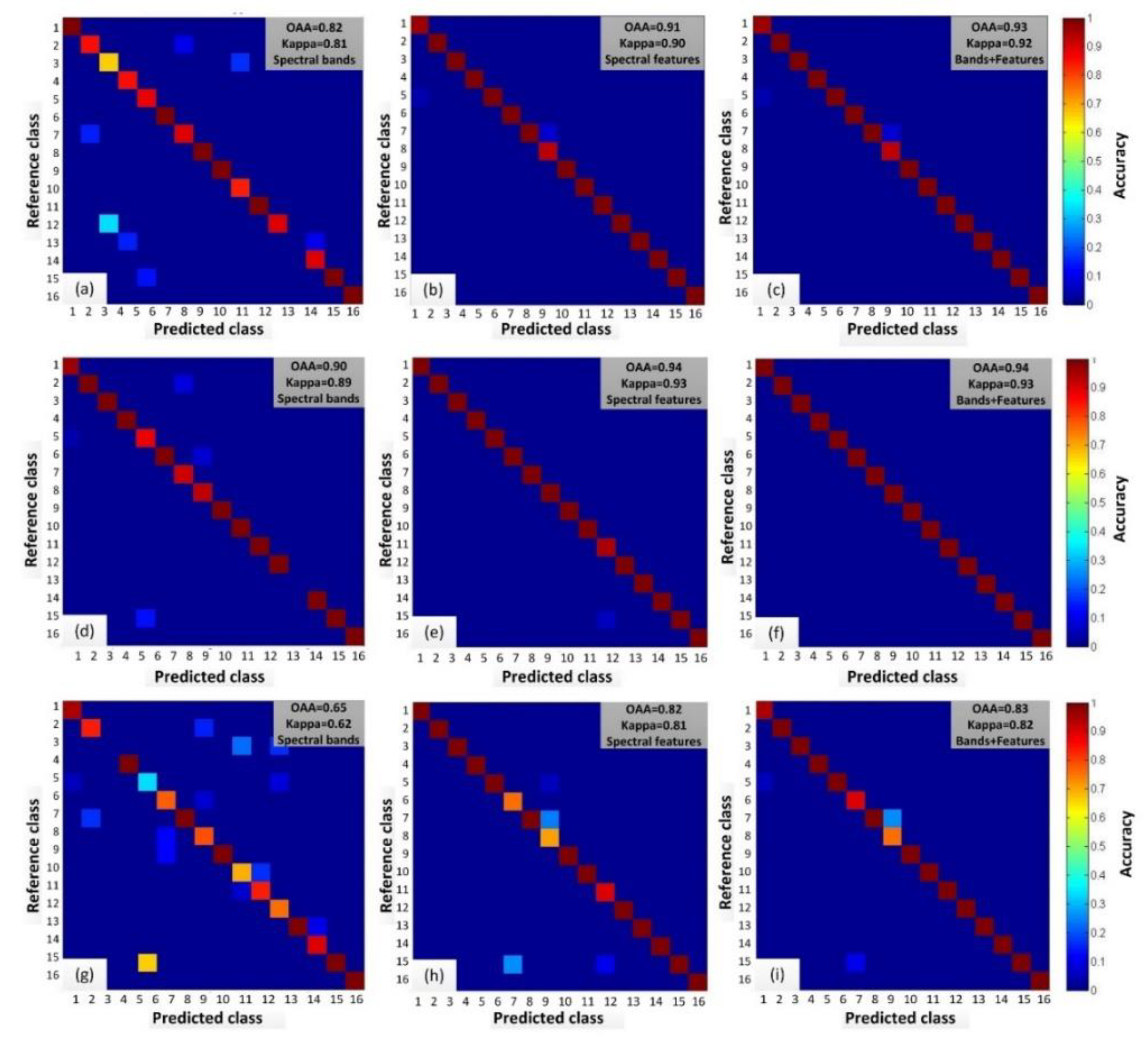
The optimized spectral features for crop classification can be categorized as follows: spectral bands, spectral features, bands + features. In order to test crop classification in a real landscape, we established a classification model that incorporated data on all 87 plant species (i.e., 16 crops + 71 non-crop plants) and then evaluated the model’s classification accuracy for 16 crops. Figure 5 shows the classification results and accuracy evaluation of the three classifiers (in the form of a confusion matrix heat map).

Spectral bands used alone consistently produced the lowest accuracy, whereas bands + features produced the highest accuracy. Spectral features used alone produced slightly lower accuracy than bands + features, suggesting that the combination of the two types of features enhances or amplifies the sensitive information of certain plants in the spectrum. Such a pattern is apparent in the classification of the Camellia yuhsienensis Hu (crop no. 13 crop in Figure 5), which was barely classified using spectral bands alone, but was clearly classified using spectral features or both types of features. In terms of the crop classification performance of different classifiers, the GA-SVM outperformed RF and KNN under all feature combinations. KNN performed significantly poorer than the other classifiers. This may be due to KNN’s simple and straightforward analytical principle, which was insufficient for handling the relatively complex scenario examined in this study. However, based on the “no-free-lunch-theorem” raised by Wolpert [49], classifier performance is probably also case sensitive. This suggests that it is necessary to perform an independent test to identify optimal algorithms when attempting to classify crops mixed with non-crop species. Here, we created a spectral library that included 16 crop species and 71 non-crop species and used it to simulate crop classification in an actual setting. Our feature sensitivity analysis identified the spectral features that reflect differences in plant categories. An optimized machine learning algorithm was then used to improve plant classification accuracy. The results demonstrate that the plant spectral library can be used for accurate crop classification.

3.3. Spectral Library-Based Crop Growing Status Monitoring

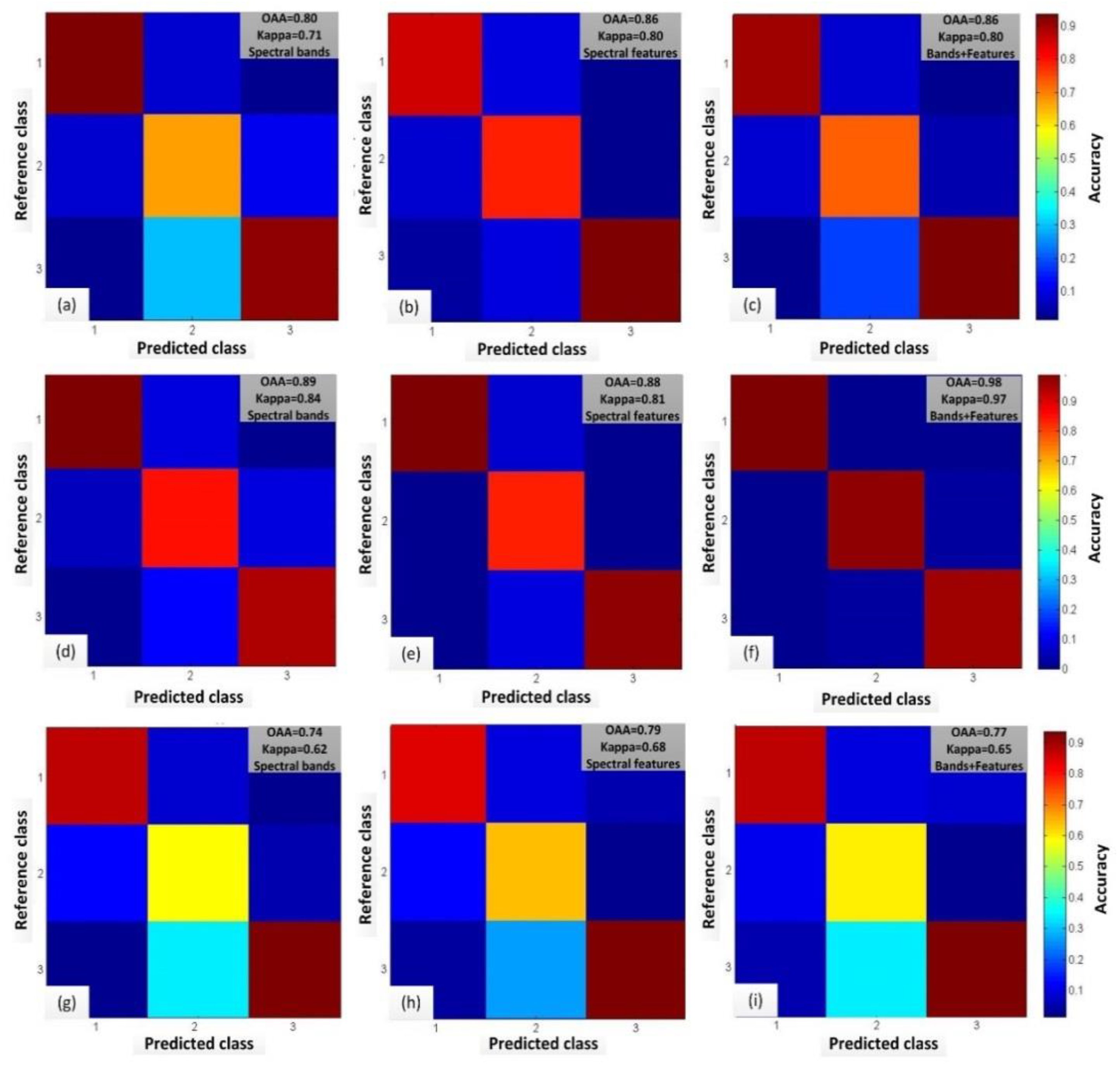
The same feature combination method was used for crop growth status monitoring as was used for crop classification to investigate the performance of the different classifiers. Figure 6 and Figure 7 show the precision of the different classification models for tea plant growth vigor and rice growth stage, respectively.

Table 6. Classification accuracy of all the spectral library-based application scenarios.

Application Scene	Feature Selected	RF		GA-SVM		KNN
		OAA	KAPPA	OAA	KAPPA	OAA	KAPPA
Crop classification	Spectral bands	0.82	0.81	0.90	0.90	0.65	0.62
	Spectral features	0.91	0.90	0.94	0.93	0.82	0.81
	Band + Features	0.93	0.92	0.94	0.93	0.83	0.82
Growth monitoring of tea trees	Spectral bands	0.80	0.71	0.89	0.84	0.74	0.62
	Spectral features	0.86	0.80	0.88	0.81	0.79	0.68
	Band + Features	0.86	0.79	0.98	0.97	0.77	0.65
Growth stage monitoring of rice	Spectral bands	0.76	0.70	0.88	0.85	0.71	0.64
	Spectral features	0.87	0.83	0.92	0.90	0.79	0.74
	Band + Features	0.85	0.81	0.92	0.90	0.77	0.71

summarizes classification accuracy of all the spectral library-based application scenarios, model accuracy depended on the type and combination of features used. For rice growth stage, models based on spectral bands alone were the least accurate and models based on spectral features alone were the most accurate. Models based on both features were slightly less accurate than those based on index features alone, which indicates a certain extent of over-fitting. In contrast, in the case of the GA-SVM classifier for tea plant growth monitoring, the accuracies of models based on spectral bands or spectral features alone were similar, whereas the highest accuracy (OAA = 0.98, Kappa = 0.97) was obtained by using both types of features. This demonstrates that spectral bands and spectral features can complement each other and improve classification accuracy. The overall comparison of the three algorithms was similar to that for plant classification. Regardless of the monitoring scenario, GA-SVM was the most accurate classification model.

In this study, we used the sensitive spectral features of tea plants in three different growth stages and rice in five different growth stages and combined the data with an optimized machine learning algorithm to build a model with high classification accuracy. This enabled effective monitoring of the growth vigor of tea plants and growth stage of rice and demonstrates the feasibility of applying a crop spectral library in crop status monitoring.

4. Conclusions

This study based on hyperspectral measurements of crops proposes the construction and application of a crop spectral library for crop classification and growth status monitoring. The following conclusions could be achieved: (1) The spectral library-based crop classification and growing status monitoring are feasible. (2) ISODATA, JM distance, correlation analysis, and strict feature screening methods can be used to identify sensitive spectral features suitable for crop classification, tea plant growth vigor monitoring, and rice growth stage monitoring. (3) The use of different feature combinations and classifier selections affect the accuracy of crop classification and status monitoring. This study tested three types of machine learning classifiers, including KNN, RF, and GA-SVM, and found that crop classification based on spectral features and GA-SVM achieved the highest classification accuracy (OAA = 0.94, Kappa = 0.93). In terms of crop growth status monitoring, the use of Bands + Features and GA-SVM achieved the highest classification accuracy for both the tea plant growth vigor monitoring (OAA = 0.98, Kappa = 0.97) and rice growth stage monitoring (OAA = 0.92, Kappa = 0.90).

The approaches presented in this study provide broad support for remote sensing-based monitoring of crops at large scales. The emergence of UAV-mounted hyperspectral cameras enables flexible and affordable acquisition of hyperspectral images. In addition, currently operational and future satellite hyperspectral sensors (e.g., CHRIS, HyspIRI, GF-5) provide an important opportunity for implementing crop species mapping and crop growth status monitoring over large areas. Future research should focus on further testing and evaluation of spectral library-based crop monitoring technologies that use UAV and satellite hyperspectral images to support large scale agricultural monitoring and administration.

References

- Campos-Taberner, M.; García-Haro, F.J.; Confalonieri, R.; Martínez, B.; Busetto, L. Multitemporal Monitoring of Plant Area Index in the Valencia Rice District with PocketLAI. Remote Sens. Environ. 2016, 8, 202. [Google Scholar] [CrossRef]
- Du, M.; Noguchi, N. Monitoring of Wheat Growth Status and Mapping of Wheat Yield’s Within-Field Spatial Variations Using Color Images Acquired from UAV-camera System. Remote Sens. Environ. 2017, 9, 289. [Google Scholar] [CrossRef]
- Jin, X.; Kumar, L.; Li, Z.; Xu, X.; Yang, G.; Wang, J. Estimation of Winter Wheat Biomass and Yield by Combining the AquaCrop Model and Field Hyperspectral Data. Remote Sens. Environ. 2016, 8, 972. [Google Scholar] [CrossRef]
- Pu, R. Hyperspectral Remote Sensing: Fundamentals and Practices; CRC Press: Boca Raton, USA, 2017. [Google Scholar]
- Adão, T.; Hruška, J.; Pádua, L.; Bessa, J.; Peres, E.; Morais, R.; Sousa, J. Hyperspectral Imaging: A Review on UAV-Based Sensors, Data Processing and Applications for Agriculture and Forestry. Remote Sens. 2017, 9, 1110. [Google Scholar] [CrossRef]
- Pu, R.; Liu, D. Segmented canonical discriminant analysis of hyperspectral data for identifying 13 urban tree species. Int. J. Remote Sens. 2011, 32, 2207–2226. [Google Scholar] [CrossRef]
- Underwood, E.C.; Ustin, S.L.; Ramirez, C.M. A Comparison of Spatial and Spectral Image Resolution for Mapping Invasive Plants in Coastal California. J. Environ. Manag. 2007, 39, 63–83. [Google Scholar] [CrossRef] [PubMed]
- Underwood, E.; Ustin, S.; Dipietro, D. Mapping nonnative plants using hyperspectral imagery. Remote Sens. Environ. 2003, 86, 150–161. [Google Scholar] [CrossRef]
- Jin, H.; Sun, Y.H.; Wang, M.Y.; Zhang, D.D.; Sada, R.; Li, M.C. Juvenile tree classification based on hyperspectral image acquired from an unmanned aerial vehicle. Int. J. Remote Sens. 2017, 38, 2273–2295. [Google Scholar]
- Yuan, H.; Yang, G.; Li, C.; Wang, Y.; Liu, J.; Yu, H.; Feng, H.; Xu, B.; Zhao, X.; Yang, X. Retrieving Soybean Leaf Area Index from Unmanned Aerial Vehicle Hyperspectral Remote Sensing: Analysis of RF, ANN, and SVM Regression Models. Remote Sens. 2017, 9, 309. [Google Scholar] [CrossRef]
- Backhaus, A.; Bollenbeck, F.; Seiffert, U. Robust classification of the nutrition state in crop plants by hyperspectral imaging and artificial neural networks. In Proceedings of the 3rd Workshop on Hyperspectral Image and Signal Processing: Evolution in Remote Sensing (WHISPERS), Lisbon, Portugal, 6–9 June 2011. [Google Scholar]
- Senthilnath, J.; Omkar, S.N.; Mani, V.; Karnwal, N.; Shreyas, P.B. Crop Stage Classification of Hyperspectral Data Using Unsupervised Techniques. IEEE J. Sel. Top. Appl. Earth Obs. Remote Sens. 2013, 6, 861–866. [Google Scholar] [CrossRef]
- Duarte-Carvajalino, J.; Alzate, D.; Ramirez, A.; Santa, J.; Fajardo-Rojas, A.; Soto-Suárez, M. Evaluating Late Blight Severity in Potato Crops Using Unmanned Aerial Vehicles and Machine Learning Algorithms. Remote Sens. 2018, 10, 1513. [Google Scholar] [CrossRef]
- Baldridge, A.M.; Hook, S.J.; Grove, C.I.; Rivera, G. The ASTER spectral library version 2.0. Remote Sens. Environ. 2009, 113, 711–715. [Google Scholar] [CrossRef]
- Nidamanuri, R.R.; Zbell, B. Transferring spectral libraries of canopy reflectance for crop classification using hyperspectral remote sensing data. Biosyst. Eng. 2011, 110, 231–246. [Google Scholar] [CrossRef]
- Baret, F.; Guyot, G. Potentials and limits of vegetation indices for LAI and APAR assessment. Remote Sens. Environ. 1991, 35, 161–173. [Google Scholar] [CrossRef]
- Zarco-Tejada, P.; Berjón, A.; Lopez-Lozano, R.; Miller, J.; Martín, P.; Cachorro, V.; González, M.R.; de Frutos, A. Assessing vineyard condition with hyperspectral indices: Leaf and canopy reflectance simulation in a row-structured discontinuous canopy. Remote Sens. Environ. 2005, 99, 271–287. [Google Scholar] [CrossRef]
- Qi, J.; Chehbouni, A.; Huete, A.R.; Kerr, Y.H.; Sorooshian, S.S. A modified soil adjusted vegetation index. Remote Sens. Environ. 1994, 48, 119–126. [Google Scholar] [CrossRef]
- Rouse, J.W.; Haas, R.H.; Schell, J.A.; Deering, D.W. Monitoring Vegetation Systems in the Great Plains with ERTS. In NASA. Goddard Space Flight Center; Texas A&M Univniversity: College Station, TX, USA, 1973. [Google Scholar]
- Koppe, W.; Fei, L.; Gnyp, M.L.; Miao, Y.; Bareth, G. Evaluating Multispectral and Hyperspectral Satellite Remote Sensing Data for Estimating Winter Wheat Growth Parameters at Regional Scale in the North China Plain. Photogramm Fernerkun 2010, 2010, 167–178. [Google Scholar] [CrossRef] [Green Version]
- Blackburn, G.A. Quantifying Chlorophylls and Caroteniods at Leaf and Canopy Scales: An Evaluation of Some Hyperspectral Approaches. Remote Sens. Environ. 1998, 66, 273–285. [Google Scholar] [CrossRef]
- Schlerf, M.; Atzberger, C.; Hill, J. Remote sensing of forest biophysical variables using HyMap imaging spectrometer data. Remote Sens. Environ. 2005, 95, 177–194. [Google Scholar] [CrossRef] [Green Version]
- Delalieux, S.; Somers, B.; Hereijgers, S.; Verstraeten, W.W.; Keulemans, W.; Coppin, P. A near-infrared narrow-waveband ratio to determine Leaf Area Index in orchards. Remote Sens. Environ. 2008, 112, 3762–3772. [Google Scholar] [CrossRef]
- Vincini, M.; Frazzi, E.; D Alessio, P. Angular dependence of maize and sugar beet VIs from directional CHRIS/PROBA data. In Proceedings of the 4th ESA CHRIS PROBA Workshop, ESRIN, Frascati, Italy, 19–21 September 2006. [Google Scholar]
- Gamon, J.A.; Peñuelas, J.; Field, C.B. A narrow-waveband spectral index that tracks diurnal changes in photosynthetic efficiency. Remote Sens. Environ. 1992, 41, 35–44. [Google Scholar] [CrossRef]
- Gitelson, A.A.; Merzlyak, M.N.; Chivkunova, O.B. Optical properties and nondestructive estimation of anthocyanin content in plant leaves. J. Photochem. Photobiol. B-Biol. 2001, 74, 38–45. [Google Scholar] [CrossRef]
- Gitelson, A.A.; Merzlyak, M.N. Signature Analysis of Leaf Reflectance Spectra: Algorithm Development for Remote Sensing of Chlorophyll. J. Plant. Physiol. 1996, 148, 494–500. [Google Scholar] [CrossRef]
- Gitelson, A.A. Remote estimation of canopy chlorophyll content in crops. Geophys. Res. Lett. 2005, 32, L08403. [Google Scholar] [CrossRef]
- Gitelson, A.A.; Kaufman, Y.J.; Stark, R.; Rundquist, D. Novel algorithms for remote estimation of vegetation fraction. Remote Sens. Environ. 2002, 80, 76–87. [Google Scholar] [CrossRef] [Green Version]
- Datt, B. A New Reflectance Index for Remote Sensing of Chlorophyll Content in Higher Plants: Tests using Eucalyptus Leaves. J. Plant. Physiol. 1999, 154, 30–36. [Google Scholar] [CrossRef]
- Daughtry, C.S.T.; Walthall, C.L.; Kim, M.S.; Colstoun, E.B.D.; McMurtrey III, J.E. Estimating Corn Leaf Chlorophyll Concentration from Leaf and Canopy Reflectance. Remote Sens. Environ. 2000, 74, 229–239. [Google Scholar] [CrossRef]
- Peñuelas, J.; Gamon, J.A.; Fredeen, A.L.; Merino, J.; Field, C.B. Reflectance indices associated with physiological changes in nitrogen- and water-limited sunflower leaves. Remote Sens. Environ. 1994, 48, 135–146. [Google Scholar] [CrossRef]
- Nagler, P.L.; Daughtry, C.S.T.; Goward, S.N. Plant Litter and Soil Reflectance. Remote Sens. Environ. 2000, 71, 207–215. [Google Scholar] [CrossRef]
- Serrano, L.; Peñuelas, J.; Ustin, S.L. Remote sensing of nitrogen and lignin in Mediterranean vegetation from AVIRIS data: Decomposing biochemical from structural signals. Remote Sens. Environ. 2002, 81, 355–364. [Google Scholar] [CrossRef]
- Galvao, L.S.; Formaggio, A.R.; Tisot, D.A. Discrimination of sugarcane varieties in Southeastern Brazil with EO-1 Hyperion data. Remote Sens. Environ. 2005, 94, 523–534. [Google Scholar] [CrossRef]
- Hardisky, M.; Klemas, V.; Smart, R.M. The influence of soil salinity, growth form, and leaf moisture on the spectral radiance of Spartina Alterniflora canopies. Photogramm. Eng. Remote Sens. 1983, 49, 77–84. [Google Scholar]
- Gao, B. NDWI–A Normalized Difference Water Index for Remote Sensing of Vegetation Liquid Water from Space. Remote Sens. Environ. 1996, 58, 257–266. [Google Scholar] [CrossRef]
- Pu, R.; Ge, S.; Kelly, N.M.; Gong, P. Spectral absorption features as indicators of water status in coast live oak (Quercus agrifolia) leaves. Int. J. Remote Sens. 2003, 24, 1799–1810. [Google Scholar] [CrossRef]
- Fensholt, R.; Sandholt, I. Derivation of a shortwave infrared water stress index from MODIS near–and shortwave infrared data in a semiarid environment. Remote Sens. Environ. 2003, 87, 111–121. [Google Scholar] [CrossRef]
- Peñuelas, J.; Pinol, J.; Ogaya, R.; Filella, I. Estimation of Plant Water Concentration by the Reflectance Water Index WI (R900/R970). Int. J. Remote Sens. 1997, 18, 2869–2875. [Google Scholar] [CrossRef]
- Ball, G.H.; Hall, D.J. ISODATA, A Novel Method of Data Analysis and Pattern Classification; Stanford Research Institute: Menlo Park, CA, USA, 1965. [Google Scholar]
- Swain, P.H.; Davis, S.M. Remote Sensing: The Quantitative Approach. IEEE Trans. Pattern Anal. Mach. Intell. 1981, 6, 713–714. [Google Scholar] [CrossRef]
- Hastie, T.; Tibshirani, R.; Friedman, J. The Elements of Statistical Learning: Data Mining, Inference, and Prediction; Springer: New York, NY, USA, 2009; pp. 459–483. [Google Scholar]
- Pal, M. Random forest classifier for remote sensing classification. Int. J. Remote Sens. 2005, 26, 217–222. [Google Scholar] [CrossRef]
- Belgiu, M.; Drăguţ, L. Random forest in remote sensing: A review of applications and future directions. Isprs-J. Photogramm. Remote Sens. 2016, 114, 24–31. [Google Scholar] [CrossRef]
- Chi, M.; Feng, R.; Bruzzone, L. Classification of hyperspectral remote-sensing data with primal SVM for small-sized training dataset problem. Adv. Space Res. 2008, 41, 1793–1799. [Google Scholar] [CrossRef]
- Congalton, R.G.; Mead, R.A. A quantitative method to test for consistency and correctness in photo-interpretation. Photogramm. Eng. Remote Sens. 1983, 49, 69–74. [Google Scholar]
- Curran, P.J. Remote sensing of foliar chemistry. Remote Sens. Environ. 1989, 30, 271–278. [Google Scholar] [CrossRef]
- Wolpert, D.H. The Lack of A Priori Distinctions Between Learning Algorithms. Neural Comput. 1996, 8, 1341–1390. [Google Scholar] [CrossRef]
Figure 1.
Examples of tea plant growth status in the study area (poor growth (a), medium growth (b), and good growth (c), respectively).
Figure 2.
(a) Canopy spectra of sixteen crops; (b) the results of band JM distance ISODATA clustering. (The species ID is referred from the Table A1. The same color indicates the same cluster.).
Figure 3.
(a) Canopy spectra for different tea plant growth stages; (b) the results of band JM distance ISODATA clustering. The same color indicates the same cluster.
Figure 4.
(a) Canopy spectra for different rice growth stages; (b) the results of band JM distance ISODATA clustering. The same color indicates the same cluster.
Figure 5.
Visualization of crop classification results using a confusion matrix heat map. ((a–c) are results using RF, (d–f) are results using GA-SVM, and (g–i) are results using K-nearest neighbors (KNN)).
Figure 6.
Visualization of tea plant growth vigor monitoring results using a confusion matrix heat map. ((a–c) are results using RF, (d–f) are results using GA-SVM, and (g–i) are results using KNN).
Figure 7.
Visualization of rice growth stage monitoring results using a confusion matrix heat map. ((a–c) are results using RF, (d–f) are results using GA-SVM, and (g–i) are results using KNN.).