Does Harvesting Affect the Spatio-Temporal Signature of Pests and Natural Enemies in Alfalfa Fields?

Abstract

Determining the spatio-temporal distribution and association of pests and natural enemies would be useful for implementing biological control of pests and could also be used in site-specific pest management. In this study, the spatio-temporal distribution and association of aphids, plant bugs, and natural enemies were assessed in alfalfa fields using geo-statistics and spatial analysis by distance indices (SADIE). Additionally, the effect of alfalfa hay-harvesting on the spatial and temporal distribution of these insects was investigated for the first time. Geostatistical analysis indicated that the degree of dependence (DD) was ≥75% for 11 out of 39, 9 out of 35, 3 out of 12, 10 out of 29, and 2 out of 20 datasets for pea aphid Acyrthosiphon pisum, spotted alfalfa aphid Therioaphis maculata, cowpea aphid Aphis craccivora, alfalfa plant bug Adelphocoris lineolatus, and tarnished plant bug Lygus rugulipennis, respectively. The results also indicated that DD was ≥75% in 7 out of 45, 18 out of 45, and 3 out of 20 datasets for Coccinella septempunctata, Hippodamia variegata, and Pterostichus melanarius, respectively. Harvesting decreased the aggregation of the ladybirds, which resulted in a decrease in the index of aggregation. The geo-statistics results were confirmed by SADIE in 75% of datasets. These results can be used in biological control and site-specific management of aphids and plant bugs in alfalfa fields.

1. Introduction

Alfalfa Medicago sativa L., is one of the earliest plants to be domesticated by humans and plays an important role in the quality of dairy products. Alfalfa fields typically have a rich insect fauna and they are suitable habitats for a large number of pests and beneficial insects. Different species of aphids are important pests in alfalfa fields in Iran. Aphid damage starts at the end of March and continues through the spring. Populations decrease during the summer due to high temperatures and increase again in the autumn [1]. Severe aphid infestation stunts plant growth and reduces yield and may even kill alfalfa plants. Aphids also produce large amounts of honeydew and make the alfalfa plants sticky, which causes problems during harvest [2,3]. Aphid populations are controlled by natural enemies in alfalfa fields and, usually, no specific chemical is applied to control them, unless the population is very high.

Tarnished plant bug, Lygus rugulipennis (Popp.), and alfalfa plant bug, Adelphocoris lineolatus (Goeze), are reported as noxious pests of several crops worldwide. Both are polyphagous, which are highly mobile and establish high population densities on various plants, and cause damage by feeding [4]. They feed on buds, flowers, and developing alfalfa seeds and reduce alfalfa production [5].

Alfalfa fields are also suitable habitats for beneficial insects such as ladybird beetles, green lacewings, ground beetles, and parasitoid wasps, which all play an important role in controlling insect pests [6]. Coccinella septempunctata L. and Hippodamia variegata (Goeze) are important biological control agents against aphids. Most of the time, these two species can be seen simultaneously in the alfalfa fields.

Determining the spatio-temporal distribution pattern of organisms is one of the most fundamental measures required to provide important information about their population dynamics and dispersal ecology. The spatial distribution patterns of insects have been investigated in many studies using different methods including variance—mean indices and spatially explicit tools such as geo-statistics and spatial analysis by distance indices (SADIE). Geo-statistics is a collection of statistical methods analyzing spatial dependence among samples (autocorrelation) and obtaining estimates of the variable under study at unsampled locations [7]. SADIE is another technique used for determining the spatial patterns of insect populations and assessing the spatial association between two sets of counts when they are sampled from identical locations. SADIE is based on the quantification of spatial patterns by using two indices known as "distance to regularity" and "distance to crowding." The former is the minimum effort that the individuals in a sample would need to expend to move to an arrangement where there was an equal number in each sample unit, and the latter is the minimum effort that the individuals in a sample would need to expend to move to an arrangement where all were crowded in the same sample unit [8]. These spatial analysis methods have been used by many researchers to determine spatial distribution patterns of different insect species: De Luigi et al. [9], Karimzadeh et al. [10,11], Reay-Jones [12,13], and Martins et al. [14] used geo-statistics or SADIE to determine the spatial distribution patterns of insect pests in maize, wheat, alfalfa, and open-field tomatoes. Park and Obrycki [15], Winder et al. [16,17], Rakhshani et al. [18], Rahman et al. [19], Diaz et al. [20], and Shayestehmehr et al. [21] also studied spatio-temporal distribution patterns and association of different species of aphids and their natural enemies in field crops using SADIE and geo-statistics.

Any information about the spatio-temporal distribution and association of pests and natural enemies in alfalfa fields would be useful for implementing biological control of pests in this crop and could also be used in site-specific pest management. Consequently, field studies are needed to determine insects’ spatio-temporal dynamics using georeferenced sampling points from alfalfa fields. Therefore, in this study, we aimed to investigate the spatio-temporal distribution and association of aphids, plant bugs, and natural enemies in alfalfa fields using geo-statistics and SADIE and compare the results of the two methods. In particular, we focused on the effect of the alfalfa harvest on the spatio-temporal distribution of both pests and natural enemies for the first time.

2. Materials and Methods

2.1. Study Site

The study was conducted in six alfalfa fields, located in the experimental farm of the Faculty of Agriculture, University of Tabriz, during the 2016 and 2017 growing seasons (Fields A, B, and C in the first year and Fields D, E, and F in the second year). The characteristics of the fields are shown in

Table 1. Characteristics of the fields in this study.

Year	Field Name	Field Area (Hectare)	Number of 20 × 20 m Grids	Number of 5 × 5 m Grids	Total Number of Grids
2016	A	1.8	42	-	42
	B	1.4	30	-	30
	C	2	46	-	46
2017	D	1.2	36	48	84
	E	1.4	33	48	81
	F	0.7	20	48	68

. In April 2014, all the fields were planted with Ghara Yonja, which is a cultivar native to Iran’s East Azarbaijan Province. Alfalfa hay was harvested four times each year in these fields. No insecticide was used in the fields during the study. Regular grids were used for sampling and all fields were divided into 20 × 20 m grids. Field borders and the spatial locations of the samples and traps were georeferenced and saved using a hand-held GPS receiver (Model GPS-map 76CSx, Garmin, Olathe, KS, USA) with the UTM (Universal Transverse Mercator) coordinate system. In order to determine insect-distribution patterns at a smaller scale, three 20 × 20 m grids with the highest insect population density were selected in fields D, E, and F, and divided into 16 smaller 5 × 5 m grids. Sampling methods in the smaller grids were similar to 20 × 20 m grids.

2.2. Sampling Methods

Sampling of the studied insects was conducted weekly from 4 July to 30 August in 2016. For carabids only, it was continued until 15 October. All target insects were sampled every week from 13 May to 25 September in 2017. Sampling was stopped at hay-cutting (harvest) time, and started again when the height of alfalfa plants reached about 10 cm.

In order to sample the aphids, 20 stems were considered as the sample unit. This number of stems were cut randomly from each grid and shaken into a white pan. The aphids that fell into the pan were counted and recorded. Coccinellids were sampled using a 1 × 1 m quadrat. Two quadrats (as the sample unit) were thrown at each grid randomly and adults, pupae, and larvae of all ladybird beetle species were counted and recorded separately. The number of insects counted in the two quadrats were pooled and used in the analysis. Plant bugs were sampled using a sweep net (38 cm diameter ring and 80 cm light wooden handle). Six to eight 180° sweeps per grid was considered as a sampling unit. Slender plastic bottles (12 cm diameter and 14 cm high) were used as pitfall traps for sampling carabids (one trap per grid). Each trap contained 200 ml water and 200 ml ethylene glycol. Carabids captured by pitfall traps were counted every two weeks and transferred to the laboratory for identification.

2.3. Spatial Analysis

Geo-statistics and SADIE were used in this study to determine the spatio-temporal distribution of insects. Geostatistical analysis was conducted using Gs⁺ version 5.1 (Gamma Design Software, Plainwell, MI, USA). Field B was excluded from geostatistical analysis since it contained too few sampling points, which are not enough for constructing valid variograms. Before autocorrelation analysis, the frequency distribution and other statistical parameters of the data were tested using the classical descriptive statistics of Gs⁺ and logarithmic transformation was used to normalize the data. Variograms were used to model the changes in spatial correlation with increasing distance between samples. To construct a variogram, the semi-variance values of paired samples were plotted against the separation distance between them [7,22]. Semi-variance was calculated using the following formula.

$$\widehat{\mathsf{\gamma }}\left(h\right)=\frac{1}{2\mathrm{N}\left(\mathrm{h}\right)}{{\displaystyle \sum }}_{\mathrm{i}=1}^{\mathrm{N}\left(\mathrm{h}\right)}{\left[\mathrm{Z}\left(x_i\right)-\mathrm{Z}\left(x_{i + h }\right)\right]}^2$$

(1)

where $\widehat{\mathsf{\gamma }}\left(h\right)$ is the empirical semi-variance at distance h, h is the distance between sample pairs or lag size, and N(h) is the number of sample pairs separated by h. Z(x_i) and Z(x_i+h) are sample values at two sample sites. Theoretical models were then fitted to the empirical variograms. The sill, partial sill, range, and nugget of the models were used to explain the spatial correlations. The patterns of directional effects or anisotropic variograms were calculated for all datasets in four directions (0, 45, 90, and 135 degrees) with 22.5-degree offset tolerance. The anisotropy factor (AF), which is the quotient between the minor and major anisotropy axes, was used to determine the existence of directional effects. Where AF was <0.5, anisotropy was considered in the analysis [23].

The residual sum of squares (RSS) was used to choose the best fitted models. Models with minimum RSS values were chosen [23,24]. Data that did not fit any model were excluded from analysis. The strength of spatial autocorrelation was measured using the degree of dependence (DD) index, defined as the ratio between partial sill and sill values of the variogram, and calculated using this formula.

$$\mathrm{DD}=\left(\frac{\mathrm{C}}{{\mathrm{C}}_0+\mathrm{C}}\right)100$$

(2)

where C₀ is the nugget, C is the partial sill, and C₀ + C is the sill of the model. Spatial dependency is low when the DD value is below 25%, since the DD approaches 75% when the level of spatial dependence will increase. This becomes high at values above 75% [25].

SADIE was also used to determine the spatial distribution of the insects and the results were compared with the results of the geostatistical analysis. The spatial pattern was investigated by calculating the index of aggregation (I_a) based on the distance to regularity. A value of I_a = 1 indicates a random spatial distribution, I_a > 1 reveals an aggregated pattern, and I_a < 1 indicates a regular or uniform spatial distribution. The probability level of I_a, (P_a) was used to determine the statistical significance of aggregation [8,26,27]. SADIE analyses were conducted using SADIE Shell, version 2.0 (Rothamsted Experimental Station, Harpenden Herts, United Kingdom).

In order to determine the effects of harvest on the spatial distribution of insects, the mean value of the I_a of all fields was calculated for each sampling date and plotted against harvest dates on coordinate axes.

2.4. Spatial Associations

The spatial association between different species sampled in this study was evaluated, including aphids, plant bugs, coccinellids, and carabids. The index of local spatial association (x_k) was calculated based on the similarity of clustering indices of the two populations at unit k using the following equation [16,28].

$$x_k=n\left(z_{k1}-q_1\right)\left(z_{k2}-q_2\right)/\sqrt{{\sum }_k{\left(z_{k1}-q_1\right)}^2{\sum }_k{\left(z_{k2}-q_2\right)}^2}$$

(3)

where x_k is the local spatial association for unit k, z_k1 and z_k2 are the clustering indices, q₁ and q₂ are the means of populations 1 and 2, respectively, and n is the total number of units. The overall spatial association (X), the mean of all x_k local values, was also calculated (formula below) and used to determine association or dissociation between species.

$$X={\sum }_i{x}_i/n_i$$

(4)

The significance of X was tested using its associated probability values (P_X). Values of X > 0 having P_X < 0.025 indicated a significant positive association, and X < 0 having P_X > 0.975 was indicative of a significant negative association or dissociation between insects [28]. Spatial association analysis was conducted using the software N-Ashell version 1.0 (Rothamsted Experimental Station, Harpenden Herts, United Kingdom).

3. Results

The data for six fields on 63 sampling dates were analyzed in this two-year study. Three species of aphids, including spotted alfalfa aphid Therioaphis maculata (Buckton), cowpea aphid Aphis craccivora (Koch), and pea aphid Acyrthosiphon pisum (Harris) were dominant in the samples. Lygus rugulipennis and A. lineolatus were the only plant bugs observed in the fields studied. Among the coccinellids, C. septempunctata and H. variegata were dominant and included in the analysis. Due to the very low number of larvae and pupae of ladybird beetles, only the number of adults was used in the analysis. Two species of carabids, including Pterostichus melanarius L. and Harpalus rufipes (Degeer), were captured in the pitfall traps. The former was dominant and included in the analysis.

3.1. Temporal Dynamics

At the beginning of the sampling period in 2016, the T. maculata population was relatively high, but it gradually decreased toward the middle of this period. The sampling period comprises the time interval between the first and last sampling date in each year. The aphid population increased again at the end of season, without evident changes before and after harvests. A. pisum was collected in very low numbers at the beginning of the survey but a slight increase in its population was observed after harvest and this continued until the end of the sampling period. A. craccivora was observed only in the samples taken shortly after the first and second harvests (Figure 1).

In 2017, A. pisum was the first species observed in the samples, which appeared on 21 June with a peak before each harvest. Compared to A. pisum, T. maculata appeared two weeks later, which was first recorded a week before the first harvest. Its population increased gradually and reached a peak before the next harvest. Its highest seasonal peak was seen before the third harvest. Similar to the previous year, A. craccivora was observed only for a period of about three weeks. Harvesting decreased the population of all aphids in this year. Population changes for aphids, especially T. maculata and A. pisum, were synchronous in both 2016 and 2017 (Figure 1).

C. septempunctata had a population peak after the first harvest in 2016, which was followed by a gradual decrease in the middle of the sampling period. The population of H. variegata displayed no significant changes during the sampling period. Ladybird beetle populations were observed earlier in the season and changed more, with four peaks, in 2017. The temporal dynamics of two ladybird species were synchronous in 2016 and 2017. Ladybird populations decreased after harvest in both years. Coccinellid and aphid population changes and peaks seemed to be coincident in both years. Comparing the distribution graphs of the two years indicated that the temporal dynamics of aphids and coccinellids were more consistent in 2017, when compared to 2016 (Figure 1).

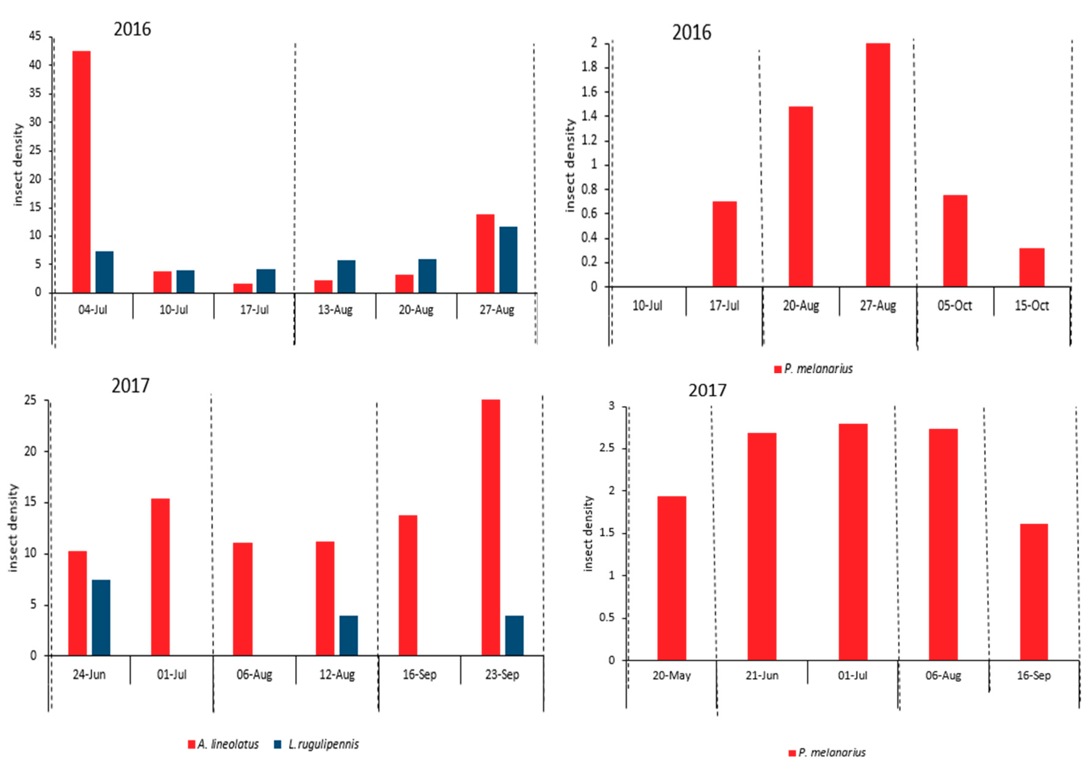
The mean number of carabids captured in the pitfall traps was low, i.e., less than three beetles per trap per sampling date, in both years. Their population was low at the beginning of the sampling period, increased slightly toward the mid-season, and then dropped late in the season. Harvest had no noticeable effect on the temporal dynamics of carabid populations (Figure 2). There was no synchrony between the temporal dynamics of aphids and P. melanarius.

In 2016, A. lineolatus and L. rugulipennis had two population peaks, at the beginning and end of the sampling period. The population of these insects peaked after the first harvest and then decreased considerably through the midseason. The second peak was observed at the end of the growing season and during the flowering period of the alfalfa plants (Figure 2). The temporal dynamics of the plant bugs was different in 2017. L. rugulipennis was present for only three short periods before harvests and A. lineolatus was not observed in the samples during the first week after harvests and its population reached a peak at the end of the season.

3.2. Geostatistical Analysis

Based on the RSS values, spherical, exponential, and Gaussian models were the best-fitted models for empirical variograms at different sampling dates. The DD was ≥75% for 11 out of 39, 9 out of 35, and 3 out of 12 datasets of A. pisum, T. maculata, and A. craccivora, respectively (

Table 2. Geostatistical degree of dependence and best -fitted variogram models for coccinellids and aphids sampling data in alfalfa fields.

Date of Sampling	Coccinalla septempunctata	Hippodamia variegata			Acyrthosiphon pisum		Therioaphis maculata		Aphis craccivora
	Field	DD	DD	Model	DD	Model	DD	Model	DD	Model
04-Jul-2016	A	-	-	No	75.4	Ex	50.1	Ex	71.9	Ex
07-Jul-2016	C	0	0	Li	99.9	Sp	99.9	Sp	-	No
10-Jul-2016	A	50	99.9	Ex	99.9	Sp	-	No	-	0
14-Jul-2016	C	-	0	Li	-	No	99.7	Sp	99.9	Sp
17-Jul-2016	A	-	99.9	Sp	-	No	-	No	-	0
19-Jul-2016	C	-	99.8	Sp	100	Ex	-	No	99.9	Sp
08-Aug-2016	A	50	99.9	Sp	-	No	-	No	-	0
09-Aug-2016	C	-	92.9	Ex	99.9	Sp	-	No	-	0
13-Aug-2016	A	75	56.8	Ex	63.5	Sp	-	No	-	0
15-Aug-2016	C	-	99.7	Sp	50	Ex	100	Sp	-	0
20-Aug-2016	A	50	98.5	Sp	84.1	Ex	99.9	Sp	-	0
22-Aug-2016	C	77.7	99.9	Ex	64.5	Ex	-	No	-	0
27-Aug-2016	A	69.6	65.8	Sp	67.1	Sp	-	No	-	0
29-Aug-2016	C	0	99.8	Ex	-	No	99.9	Sp	-	0
13-May-13	D	0	0	Li	-	0	-	0	-	0
14-May-14	E	0	0	Li	-	0	-	0	-	0
20-May-20	D	-	0	Li	-	0	-	0	-	0
21-May-21	E	50	50	Ga	-	0	-	0	-	0
27-May-27	D	-	50	Ex	-	0	-	0	-	0
28-May-28	E	51.2	50	Ga	-	0	-	0	-	0
21-Jun-21	D	-	60.3	Sp	0	Li	-	0	-	0
22-Jun-22	E	60.8	60.9	Ex	-	No	-	0	-	0
24-Jun-24	D	-	-	No	-	No	-	0	50	Ga
25-Jun-25	E	-	-	No	64.7	Sp	-	0	-	No
01-Jul-01	D	-	64.7	Sp	-	No	-	No	100	Li
02-Jul-02	E	-	99.9	Sp	50	Ga	-	No	-	No
03-Jul-03	F	61.2	81.5	Ex	89.5	Sp	-	No	-	No
30-Jul-30	D	-	-	No	75.8	Sp	-	No	-	No
31-Jul-31	E	-	-	No	-	No	-	No	50.2	Sp
01-Aug-2017	F	-	-	No	78.7	Ga	-	No	65.7	Ex
06-Aug-2017	D	-	-	No	50	Ga	-	No	-	0
07-Aug-2017	E	77	-	No	-	No	-	No	-	0
08-Aug-2017	F	99.9	99.9	Sp	-	No	50	Sp	-	0
12-Aug-2017	D	-	79.9	Ga	0	Li	50	Ga	-	0
13-Aug-2017	E	-	77.3	Sp	-	No	79.1	Ex	-	0
14-Aug-2017	F	93	100	Ex	50	Ga	92.9	Sp	-	0
10-Sep-2017	D	50	-	No	51.2	Sp	52.6	Sp	-	0
11-Sep-2017	E	-	-	No	-	No	0	Li	-	0
12-Sep-2017	F	-	-	No	50	Sp	0	Li	-	0
16-Sep-2017	D	-	-	No	-	No	-	No	-	0
17-Sep-2017	E	100	99.9	Ex	99.9	Ex	79.4	Sp	-	0
18-Sep-2017	F	83	96	Sp	-	No	-	No	-	0
23-Sep-2017	D	-	100	Ex	-	No	-	No	-	0
24-Sep-2017	E	-	-	No	-	No	-	No	-	0
25-Sep-2017	F	-	-	No	96	Sp	99.9	Ex	-	0

Ga: Gaussian model. Ex: Exponential model. Sp: Spherical model. Li: Linear model. No: no model. 0: Insect population was zero.

), which indicates that the distribution pattern of aphids was aggregated in these dates and fields. The mean range, which is an indicator of hot spot size, was 161 ± 34 m for T. maculata, 176 ± 43 m for A. craccivora, and 216 ± 26 m for A. pisum.

C. septempunctata and H. variegata showed strong spatial autocorrelation (DD ≥ 75%) in seven out of 45 and 18 out of 45 datasets, respectively. Mean ranges were 217 ± 27 m for C. septempunctata, and 178 ± 25 m for H. variegata (Table 2).

Spatial dependency was strong and DD was ≥75% for 10 out of 29, 2 out of 20, and 3 out of 20 datasets of A. lineolatus, L. rugulipennis, and P. melanarius, respectively (Supplementary Tables S1 and S2). The mean ranges were 136 ± 28 m for A. lineolatus, 223 ± 38 m for L. rugulipennis, and 261 ± 31 m for P. melanarius. After harvesting the hay, no models fitted the data or DD was less than 75% in most datasets, which means that low aggregation or a random spatial pattern was dominant after the harvest.

3.3. SADIE Analysis

According to the SADIE results, the I_a of A. pisum was >1 in 35 out of 46 datasets, which was statistically significant in 12 cases (P_a < 0.05). T. maculata and A. craccivora showed aggregated distribution in 10 out of 42 and 4 out of 16 datasets, respectively. A relatively weak aggregation was observed in the data for ladybird beetles, and the I_a of C. septempunctata and H. variegata was >1 in 30 and 34 out of total 104 datasets, and was statistically significant in 12 cases and 8 cases, respectively (

Table 3. Index of aggregation of coccinellids and aphids in alfalfa fields.

Date of Sampling	Field	Coccinalla septempunctata	Hippodamia variegata	Acyrthosiphon pisum	Therioaphis maculata	Aphis craccivora
04-Jul-2016	A	2.253 *	1.034	0.6737	1.035	1.138
05-Jul-2016	B	1.389	1.026	0.841	0.982	1.359
07-Jul-2016	C	1.530 *	1.538	1.544 *	1.523 *	1.535 *
10-Jul-2016	A	1.478	0.962	0.4493	1.303	0
12-Jul-2016	B	1.872 *	1.641 *	1.156	1.139	0.86
14-Jul-2016	C	1.395	1.393	1.35	1.395 *	1.396 *
17-Jul-2016	A	0.972	0.763	1.308	0.923	0
18-Jul-2016	B	1.497 *	1.189	1.07	0.994	0.944
19-Jul-2016	C	1.393 *	1.397 *	1.369 *	1.395 *	1.396 *
08-Aug-2016	A	0.824	1.1	1.057	1.295	0
10-Aug-2016	B	1.027	0.907	1.655 *	0.87	1.248
09-Aug-2016	C	0.972	1.124	1.144	0.896	0
13-Aug-2016	A	1.454	1.217	1.343	0.905	0
14-Aug-2016	B	0.997	0.888	1.104	0.994	0
15-Aug-2016	C	1.194	0.882	1.109	1.133	0
20-Aug-2016	A	0.935	1.701 *	2.154 *	1.769 *	0
21-Aug-2016	B	0.932	0.83	1.315	0.959	0
22-Aug-2016	C	1.463 *	0.874	1.144	0.976	0
27-Aug-2016	A	0.475	1.063	1.865 *	1.168	0
28-Aug-2016	B	0.814	0.813	0.842	1.417 *	0
29-Aug-2016	C	0.859	0.943	1.137	1.398 *	0
13-May-2017	D	0.743	0.94	0	0	0
14-May-2017	E	0.983	0.968	0	0	0
20-May-2017	D	0.874	0.7	0	0	0
21-May-2017	E	0.878	1.115	0	0	0
27-May-2017	D	0.777	1.054	0	0	0
28-May-2017	E	1.529 *	0.811	0	0	0
21-Jun-2017	D	1.203	1.11	0.715	0	0
22-Jun-2017	E	0.921	1.165	0.913	0	0
24-Jun-2017	D	0.822	0.92	0.839	0	0.783
25-Jun-2017	E	1.385	1.629 *	1.287	0	0.982
01-Jul-2017	D	1.541 *	1.795 *	1.091	0	1.815 *
02-Jul-2017	E	1.291	1.251	1.247	0	0.709
03-Jul-2017	F	1.461 *	1.597 *	1.819 *	0	1.101
30-Jul-2017	D	1.12	1.554 *	1.922 *	1.247	1.341
31-Jul-2017	E	0.921	0.87	1.52	0.958	1.345
01-Aug-2017	F	0.908	1.045	1.389 *	0.904	1.018
06-Aug-2017	D	1.540 *	1.09	0.965	1.174	0
07-Aug-2017	E	2.294 *	1.266	1.012	1.837 *	0
08-Aug-2017	F	1.044	1.044	1.23	1.456 *	0
12-Aug-2017	D	1.19	1.425	0.852	0.937	0
13-Aug-2017	E	1.064	1.56	0.816	2.228 *	0
14-Aug-2017	F	0.809	1.382	0.865	1.223	0
10-Sep-2017	D	1.098	1.11	1.319	1.095	0
11-Sep-2017	E	0.698	1.017	1.037	0.883	0
12-Sep-2017	F	1.115	0.811	1.337	0.778	0
16-Sep-2017	D	1.453	1.317	1.517 *	0.973	0
17-Sep-2017	E	1.323	1.41	2.485 *	3.793 *	0
18-Sep-2017	F	1.428 *	1.480 *	1.206	1.304	0
23-Sep-2017	D	1.086	1.132	2.427 *	1.122	0
24-Sep-2017	E	0.713	0.796	1.711 *	0.945	0
25-Sep-2017	F	0.724	0.865	1.202	1.326	0

*: Statistical significance of aggregation (p < 0.05). 0: Insect population was zero.

).

I_a values indicated that the spatial distribution pattern of A. lineolatus and L. rugulipennis was aggregated in 15 out of 35 and 4 out of 26 datasets, respectively (P_a < 0.05). The I_a calculated for the carabid P. melanarius was >1 in 15 out of 30 datasets, which was statistically significant in four cases (Supplementary Tables S2 and S3). The results of SADIE agreed with the results of geo-statistics in 75% of cases. Figure 3 and Figure 4 show the effect of harvests on the SADIE I_a. It seems that only the I_a values of ladybird beetles decreased after the harvest and this event had no significant effect on the aggregation of other species.

3.4. Spatial Associations between Species

The association index (X) indicated that there was a statistically significant positive spatial association (P_X < 0.025) between the aphids T. maculata and A. pisum on seven dates in the sampling periods at the beginning of 2016 and in the middle of 2017. Negative spatial association or dissociation between these two aphids was statistically significant (P_X > 0.975) on one date only in Field E. A. craccivora and T. maculata populations showed a strong positive association on three dates in the first sampling period of 2016. No dissociation was observed between these species. The I_a between A. craccivora and A. pisum was positive and statistically significant for three dates at the beginning of the season (Supplementary Table S4).

The spatial association index for A. pisum and H. variegata and for this aphid and C. septempunctata was statistically significant in 7 and 5 out of 96 datasets (

Table 4. Spatial association between Acyrthosiphon pisum and Coccinellids (Coccinella septempunctata and Hippodamia variegata).

Date of Sampling	Field	A. pisum and H. variegata		A. pisumand C. septempunctata
			X	Px	X	Px
04-Jul-2016	A	−0.0792	0.25	−0.2520	0.75
05-Jul-2016	B	0.2525	0.25	0.1089	0.2928
07-Jul-2016	C	1	0.0001	1	0.0001
10-Jul-2016	A	−0.0024	0.25	−0.010	0.25
12-Jul-2016	B	0.2352	0.25	0.5927	0.0284
14-Jul-2016	C	1	0.0001	1	0.0001
17-Jul-2016	A	0.2469	0.25	0.2469	0.25
18-Jul-2016	B	0.0992	0.25	−0.2374	0.901
19-Jul-2016	C	1	0.0001	1	0.0001
08-Aug-2016	A	0.818	0.25	0.0818	0.5
10-Aug-2016	B	0.2239	0.25	0.3518	0.25
09-Aug-2016	C	−0.0653	0.25	0.1	0.2661
13-Aug-2016	A	0.3072	0.25	0.3072	0.25
14-Aug-2016	B	−0.1535	0.5	0.0176	0.4505
15-Aug-2016	C	−0.1013	0.5	0.516	0.25
20-Aug-2016	A	−0.0276	0.25	0.1033	0.25
21-Aug-2016	B	0.0112	0.25	0.2332	0.1335
22-Aug-2016	C	0.3285	0.25	0.2406	0.25
27-Aug-2016	A	0.1382	0.25	0.5903	0.25
28-Aug-2016	B	0.0474	0.25	0.3643	0.0652
29-Aug-2016	C	0.6455	0.25	0.3763	0.25
21-Jun-2017	D	−0.0889	0.684	0.1322	0.2168
22-Jun-2017	E	0.11	0.2907	0.0418	0.5655
23-Jun-2017	F	0.1893	0.2399	0.4929	0.0407
24-Jun-2017	D	0.1623	0.1813	0.0443	0.3812
25-Jun-2017	E	0.1815	0.8027	−0.0864	0.6224
26-Jun-2017	F	0.4362	0.0578	−0.1289	0.6378
01- Jul-2017	D	0.0476	0.3061	0.087	0.1992
02-Jul-2017	E	−0.0242	0.5525	−0.01174	0.8503
03-Jul-2017	F	0.4505	0.0017	0.4661	0.0002
30-Jul-2017	D	0.2999	0.0063	0.1231	0.1349
31-Jul-2017	E	−0.1628	0.9508	0.0715	0.2261
01-Aug-2017	F	0.1108	0.1901	0.0684	0.2951
06-Aug-2017	D	0.2563	0.0123	−0.0949	0.8063
07-Aug-2017	E	−0.1686	0.9365	−0.2110	0.9715
08-Aug-2017	F	0.0647	0.3022	0.0647	0.3022
12-Aug-2017	D	0.0268	0.3906	0.0723	0.2609
13-Aug-2017	E	0.0081	0.4619	−0.0719	0.7255
14-Aug-2017	F	0.1772	0.1046	0.0358	0.3811
10-Sep-2017	D	−0.1039	0.8135	0.1837	0.0612
11-Sep-2017	E	−0.1343	0.8795	−0.0609	0.6781
12-Sep-2017	F	0.0411	0.3577	−0.0256	0.5613
16-Sep-2017	D	0.2088	0.0362	0.1287	0.1517
17-Sep-2017	E	0.412	0.0001	0.4397	0.0006
18-Sep-2017	F	0.2413	0.0305	0.1315	0.15
23-Sep-2017	D	−0.0362	0.5881	−0.0230	0.5364
24-Sep-2017	E	−0.513	0.6365	−0.1630	0.9392
25-Sep-2017	F	−0.1031	0.7822	0.036	0.2472

X, index of spatial association. P_X, P values of X.

). A negative association or dissociation between these species was not significant. T. maculata had a positive association with H. variegata and C. septempunctata in 9 and 8 out of 41 and 42 datasets, respectively (Supplementary Table S5).

A strong spatial association was observed between A. craccivora and H. variegata and between this aphid and C. septempunctata in four out of 16 datasets (P_X > 0.975) (

Table 5. Spatial association between Aphis craccivora and Coccinellids (Coccinella septempunctata and Hippodamia variegata).

Date of Sampling	Field	A. craccivora and H. variegata		A. craccivora and C. septempunctata
			X	Px	X	Px
04-Jul-2016	A	0.5544	0.0072	0.464	0.0043
05-Jul-2016	B	0.1327	0.1948	0.2874	0.0515
07-Jul-2016	C	1	0.0001	1	0.0001
12-Jul-2016	B	−0.0868	0.5519	−0.1920	0.8425
14-Jul-2016	C	1	0.0001	1	0.0001
18-Jul-2016	B	−0.0843	0.5525	−0.1106	0.6591
19-Jul-2016	C	1	0.0001	1	0.0001
10-Aug-2016	B	0.0911	0.3721	0.3325	0.0603
24-Jun-2017	D	−0.0984	0.6837	0.261	0.0965
25-Jun-2017	E	−0.0379	0.479	0.1394	0.1063
01-Jul-2017	D	−0.0672	0.7047	0.0651	0.2552
02-Jul-2017	E	−0.0615	0.6553	0.0057	0.3936
03-Jul-2017	F	0.095	0.2316	0.0925	0.2339
30-Jul-2017	D	0.0654	0.257	0.0397	0.3604
01-Aug-2017	F	−0.0033	0.4849	−0.1213	0.8198

X, index of spatial association. P_X, P values of X.

).

The associations between T. maculata and P. melanarius and between A. pisum and P. melanarius were statistically significant in only three out of 37 datasets (Supplementary Table S6). The spatial association index between A. craccivora and P. melanarius was not determined, because this aphid was observed in samples for a short time that did not coincide with the presence of carabids in the fields.

4. Discussion

The population of natural enemies sampled in this study was not high. As noted previously, this study was conducted at an experimental farm located in a simple landscape. The simplicity and low diversity of the agroecosystem around the fields and the lack of natural and semi-natural habitats in the area may explain the low density of natural enemies such as coccinellids and carabids in the studied fields. Several other researchers have come to similar conclusions that the simplicity of the landscape results in lower populations and diversity of natural enemies [29,30,31].

The temporal dynamics of coccinellid and aphid populations were synchronous in the two years, especially in 2017. This is important for the biological control of aphids because ladybird beetles can effectively reduce the number of aphids when their populations are coincident, spatially and temporally [15]. It should be noted that temporal synchrony of pests and natural enemies may not guarantee that spatial association will occur in the fields throughout the growing season. As seen in this study, spatial association between aphids and coccinellids was inconsistent and unstable during the growing seasons. Instability in insect spatial patterns and spatial association between pests and natural enemies has been reported by other researchers as well. Pearce and Zalucki [32] reported that predator aggregation did not consistently correlate with pest aggregation and differed between fields. Park and Obrycki [15] used map-correlation analysis to determine spatial association between aphids and coccinellids and reported that the spatial distribution of ladybirds did not always coincide with that of corn leaf aphids. Both association and dissociation were observed between aphids and their natural enemies, but on few specific dates.

Harvesting of the alfalfa crop, several times a year, could be one of the major reasons for the instability of the spatial distribution patterns of pests and natural enemies and their association in alfalfa fields. Cutting the hay during the growing season can disrupt insect distribution patterns and the insects have to rebuild their distribution patterns after the harvest. Therefore, spatial distribution patterns will be different before and after the harvest. Our results somewhat confirmed this hypothesis. Harvesting decreased the number of aphids and coccinellids but did not affect carabid populations. These results were expected, because aphids and coccinellids are located in the plant canopy and harvesting can remove some of them. In contrast, carabids live on the surface of the ground and the probability of removing them when harvesting the plants is low.

Considering the feeding behavior of L. rugulipennis, high populations were expected at the alfalfa flowering stage. The reduced population of this bug toward the end of the growing season in 2017 can be attributed to the presence of old alfalfa fields nearby. These old fields entered the flowering stage earlier than the studied fields and were at the flowering and seeding stages for a longer period of time. Therefore, more plant bugs left the studied fields for the old fields and their populations decreased in the studied fields. Sampling of the old fields confirmed this (data not presented).

The use of two spatial statistical methods, which are geo-statistics and SADIE, provided some reliable comparisons [33,34,35]. Both methods determined the spatial distribution patterns of sampled insects in the alfalfa fields, using the Degree of Dependence Index (DD) or the Index of Aggregation (Ia), respectively. SADIE was designed specifically for count-based data spatially referenced in two dimensions and has been more extensively applied to interactions between pests and their natural enemies [17]. In our study, the SADIE results overlapped with the geo-statistics in 75% of the datasets, by highlighting a good match level. SADIE, unlike the variogram analysis, provides a randomization test for significance, which returned a random pattern in a few cases when the DD index indicated an aggregated distribution.

According to the results, the spatial distribution of all studied species in the fields was not stable overall and changed over time. The pattern of these changes was specific to each insect and revealed a unique signature of that insect in that environmental condition, which is the reason for our proposing to use the term “spatio-temporal signature” instead of “spatio-temporal distribution.” In other words, each insect population has its own unique spatio-temporal signature in the field, at least when the stochastic processes of dispersion (leading to random distributions) do not prevail.

The existence of spatio-temporal associations between pests and their natural enemies is useful in implementing biological control of pests and can increase the efficiency of natural enemies. Spatial dissociation can also provide useful information for chemical control, i.e., site-specific treatments can be applied only to aphid patches or hot spots without affecting natural enemies significantly. Determining the spatio-temporal signature and association of pests and natural enemies provides useful information that can augment biological control with landscape management. For example, the strong perturbation of insect populations in the fields caused by alfalfa harvesting, disrupting interactions among pests and natural enemies, can have negative effects on the efficacy of biological control, especially with low predator populations. In this case, the increase of areas for shelter (wild vegetation strips or hedgerows) adjacent to the alfalfa fields can assume even greater importance for rapid recolonization of natural enemies within the crop.

The observed lack of association could also be due to the higher mobility of predators that show a random distribution more often than prey species. The incorporation of aspects related to dispersal processes can provide a clear causal description of the spatial patterns observed at field level.

5. Conclusions

In this study, the spatio-temporal distribution and association of aphids, plant bugs, and natural enemies were determined in alfalfa fields using geo-statistics and SADIE. Additionally, the effect of alfalfa hay-harvesting on the spatio-temporal distribution of these insects was investigated. According to the results, the spatial distribution of all studied species in the fields was not stable overall and changed over time. SADIE results agreed with the results of geo-statistics in 75% of the datasets, which highlights a good match level. Although there was a temporal synchrony between ladybird beetles and aphids, they were not spatially coincident on all dates. No noticeable spatial and temporal association was observed between aphids and carabids. Harvesting decreased populations of the aphids and ladybird beetles but had no significant effect on the number of carabids or plant bugs. It also decreased the aggregation of the ladybirds, which resulted in a decrease in the index of aggregation (I_a). The results can be used in biological control and site-specific management of pests in alfalfa fields. The existence of spatio-temporal associations between aphids and their natural enemies is useful in implementing biological control of these pests and can increase the efficiency of natural enemies. Spatial dissociation can also provide useful information for chemical control, i.e., site-specific treatments can be applied only to aphid patches or hot spots without affecting natural enemies significantly.

References

- Khanjani, M. Field Crop Pests in Iran, 2nd ed.; Bu-Ali Sina University Press: Tehran, Iran, 2005; 738p. [Google Scholar]
- Hodgson, E.W. Aphids in Alfalfa. 2007. Utah State University Extension, Logan, Utah Pests Fact Sheet, Entomology:107-07. Available online: https://utahpests.usu.edu/uppdl/files-ou/factsheet/Aphids%20in%20Alfalfa (accessed on 10 July 2007).
- Canevari, W.M.; Davis, R.M.; Frate, C.A.; Godfrey, L.D.; Goodell, P.B.; Lanini, W.T.; Long, R.F.; Natwick, E.T.; Orloff, S.; Putnam, D.H.; et al. UC IPM Pest Management Guidelines, Alfalfa. UC ANR Publication 3430. Oakland, CA. 2015. Available online: http://www.ipm.ucdavis.edu (accessed on 14 September 2015).
- Accinelli, G.; Lanzoni, A.; Ramilli, F.; Dradi, D.; Burgio, G. Trap crop: An agroecological approach to the management of Lygus rugulipennis on lettuce. B. Insectol. 2005, 58, 9–14. [Google Scholar]
- Mirab-balou, M.; Radjabi, R. Lygus rugulipennis Poppius (Hemiptera: Miridae): A key pest on alfalfa (Medicago sativa L.) in west of Iran, and checklist of the insect pests. Persian Gulf Crop Protect. 2013, 2, 57–66. [Google Scholar]
- Caballero-López, B.; Bommarco, R.; Blanco-Moreno, J.M.; Sans, F.X.; Pujade-Villar, J.; Rundlöf, M.; Smith, H.G. Aphids and their natural enemies are differently affected by habitat features at local and landscape scales. Biol. Control 2012, 63, 222–229. [Google Scholar] [CrossRef]
- Hasani Pak, M. Geostatistics; Tehran University Press: Tehran, Iran, 2007; 328p. [Google Scholar]
- Perry, J.N. Spatial aspects of animal and plant distribution in patchy farmland habitats. In Ecology and Integrated Farming Systems; Glen, D.M., Greaves, M.A., Anderson, H.M., Eds.; John Wiley & Sons: New York, NY, USA, 1995; pp. 221–242. [Google Scholar]
- De Luigi, V.; Furlan, L.; Palmieri, S.; Vettorazzo, M.; Zanini, G.; Edwards, C.R.; Burgio, G. Results of WCR monitoring plans and evaluation of an eradication programme using GIS and Indicator Kriging. J. Appl. Entomol. 2011, 135, 38–46. [Google Scholar] [CrossRef]
- Karimzadeh, R.; Hejazi, M.J.; Helali, H.; Iranipour, S.; Mohammadi, S.A. Analysis of the spatio-temporal distribution of Eurygaster integriceps (Hemiptera: Scutelleridae) by using spatial analysis by distance indices and geostatistics. Environ. Entomol. 2011, 40, 1253–1265. [Google Scholar] [CrossRef] [PubMed]
- Karimzadeh, R.; Zakeri Ilkhchi, M.; Iranipour, S. Determining spatial distribution of alfalfa leaf weevil Hypera postica and root weevils Sitona spp. (Coleoptera: Curculionidae) using geostatistics. Appl. Entomol. Phytopathol. 2015, 83, 1–13. [Google Scholar]
- Reay-Jones, F.P. Spatial distribution of stink bugs (Hemiptera: Pentatomidae) in wheat. J. Insect Sci. 2014, 14. [Google Scholar] [CrossRef]
- Reay-Jones, F.P. Geostatistical characterization of cereal leaf beetle (Coleoptera: Chrysomelidae) distributions in wheat. Environ. Entomol. 2017, 46, 931–938. [Google Scholar] [CrossRef]
- Martins, J.C.; Picanço, M.C.; Silva, R.S.; Gonring, A.H.; Galdino, T.V.; Guedes, R.N. Assessing the spatial distribution of Tuta absoluta (Lepidoptera: Gelechiidae) eggs in open-field tomato cultivation through geostatistical analysis. Pest Manag. Sci. 2018, 74, 30–36. [Google Scholar] [CrossRef]
- Park, Y.L.; Obrycki, J.J. Spatio-temporal distribution of corn leaf aphids (Homoptera: Aphididae) and lady beetles (Coleoptera: Coccinellidae) in Iowa cornfields. Biol. Control 2004, 31, 210–217. [Google Scholar] [CrossRef]
- Winder, L.; Alexander, C.J.; Holland, J.M.; Woolley, C.; Perry, J.N. Modelling the dynamic spatio-temporal response of predators to transient prey patches in the field. Ecol. Lett. 2001, 4, 568–576. [Google Scholar] [CrossRef]
- Winder, L.; Alexander, C.J.; Holland, J.M.; Symondson, W.O.; Perry, J.N.; Woolley, C. Predatory activity and spatial pattern: The response of generalist carabids to their aphid prey. J. Anim. Ecol. 2005, 74, 443–454. [Google Scholar] [CrossRef]
- Rakhshani, H.; Ebadi, R.; Mohammadi, A.A. Population dynamics of alfalfa aphids and their natural enemies, Isfahan, Iran. J. Agr. Sci. Technol. 2009, 11, 505–520. [Google Scholar]
- Rahman, T.; Roff, M.N.M.; Ghani, I.B.A. Within-field distribution of Aphis gossypii and aphidophagous lady beetles in chili, Capsicum annuum. Entomol. Exp. Appl. 2010, 137, 211–219. [Google Scholar] [CrossRef]
- Díaz, B.M.; Legarrea, S.; Marcos-García, M.Á.; Fereres, A. The spatio-temporal relationships among aphids, the entomophthoran fungus, Pandora neoaphidis, and aphidophagous hoverflies in outdoor lettuce. Biol. Control 2010, 53, 304–311. [Google Scholar] [CrossRef]
- Shayestehmehr, H.; Karimzadeh, R.; Hejazi, M.J. Spatio-temporal association of Therioaphis maculata and Hippodamia variegata in alfalfa fields. Agric. For. Entomol. 2016, 19, 81–92. [Google Scholar]
- Duarte, F.; Calvo, M.V.; Borges, A.; Scatoni, I.B. Geostatistics applied to the study of the spatial distribution of insects and its use in integrated pest management. Rev. Ciênc. Agron. 2015, 35, 9–20. [Google Scholar]
- Goovaerts, P. Geostatistics for Natural Resources Evaluation; Oxford University Press: New York, NY, USA, 1997; 483p. [Google Scholar]
- Sciarretta, A.; Trematerra, P. Geostatistical tools for the study of insect spatial distribution: Practical implications in the integrated management of orchard and vineyard pests. Plant Protect. Sci. 2014, 50, 97–110. [Google Scholar] [CrossRef]
- Grego, C.R.; Vieira, S.R.; Lourenção, A.L. Spatial distribution of Pseudaletia sequax Franclemlont in triticale under no-till management. Sci. Agric. 2006, 63, 321–327. [Google Scholar] [CrossRef]
- Perry, J.N. Spatial analysis by distance indices. J. Anim. Ecol. 1995, 64, 303–314. [Google Scholar] [CrossRef]
- Holland, J.M.; Perry, J.N.; Winder, L. The within-field spatial and temporal distribution of arthropods in winter wheat. Bull. Entomol. Res. 1999, 89, 499–513. [Google Scholar] [CrossRef]
- Perry, J.N.; Dixon, P.M. A new method to measure spatial association for ecological count data. Ecoscience 2002, 9, 133–141. [Google Scholar] [CrossRef]
- Veres, A.; Petit, S.; Conord, C.; Lavigne, C. Does landscape composition affect pest abundance and their control by natural enemies? A review. Agric. Ecosyst. Environ. 2013, 166, 110–117. [Google Scholar] [CrossRef]
- Woltz, J.; Landis, D.A. Coccinellid response to landscape composition and configuration. Agric. For. Entomol. 2014, 16, 341–349. [Google Scholar] [CrossRef]
- Jung, J.K.; Lee, J.H. Forest–farm edge effects on communities of ground beetles (Coleoptera: Carabidae) under different landscape structures. Ecol. Res. 2016, 31, 799–810. [Google Scholar] [CrossRef]
- Pearce, S.; Zalucki, M.P. Do predators aggregate in response to pest density in agroecosystems? Assessing within-field spatial patterns. J. Appl. Ecol. 2006, 43, 128–140. [Google Scholar] [CrossRef]
- Madden, L.V.; Hughes, G. Plant disease incidence: Distributions, heterogeneity, and temporal analysis. Annu. Rev. Phytopathol. 1995, 33, 529–564. [Google Scholar] [CrossRef]
- Perry, J.N.; Liebhold, A.M.; Rosenberg, M.S.; Dungan, J.; Miriti, M.; Jakomulska, A.; Citron-Pousty, S. Illustrations and guidelines for selecting statistical methods for quantifying spatial pattern in ecological data. Ecography 2002, 25, 578–600. [Google Scholar] [CrossRef] [Green Version]
- Campos-Herrera, R.; Ali, J.G.; Diaz, B.M.; Duncan, L.W. Analyzing spatial patterns linked to the ecology of herbivores and their natural enemies in the soil. Front. Plant. Sci. 2013, 4, 378. [Google Scholar] [CrossRef] [Green Version]
Figure 1.
Temporal dynamics of the coccinellids (left) and aphids (right) in the studied alfalfa fields in the first, second, third, and fourth weeks after harvest (dashed lines indicate alfalfa harvest times). Coccinellids were sampled using a 1 × 1 m quadrat and aphids counted on 20 stems were cut randomly from each grid.
Figure 2.
Temporal dynamics of the plant bugs Lygus rugulipennis and Adelphocoris lineolatus (left) and carabid Pterostichus melanarius (right) in the studied alfalfa fields in the first, second, third, and fourth weeks after harvest (dashed lines indicate alfalfa harvest times). Plant bugs and carabid were sampled using sweep nets and pitfall traps, respectively.
Figure 3.
The average of the index of aggregation (Ia) of coccinellids (left) and aphids (right) in 2016 and 2017 (dashed lines indicate alfalfa harvest times). Bars indicate standard errors.
Figure 4.
The average of the aggregation (Ia) index of plant bugs (left) and Pterostichus melanarius (right) in 2016 and 2017 (dashed lines indicate alfalfa harvest times). Bars indicate standard errors.