

Environmental and Socioeconomic Determinants of Virtual Water Trade of Grain Products: An Empirical Analysis of South Korea Using Decomposition and Decoupling Model

 ,
,  , ,
, , 

Abstract
:1. Introduction
2. Methods and Data
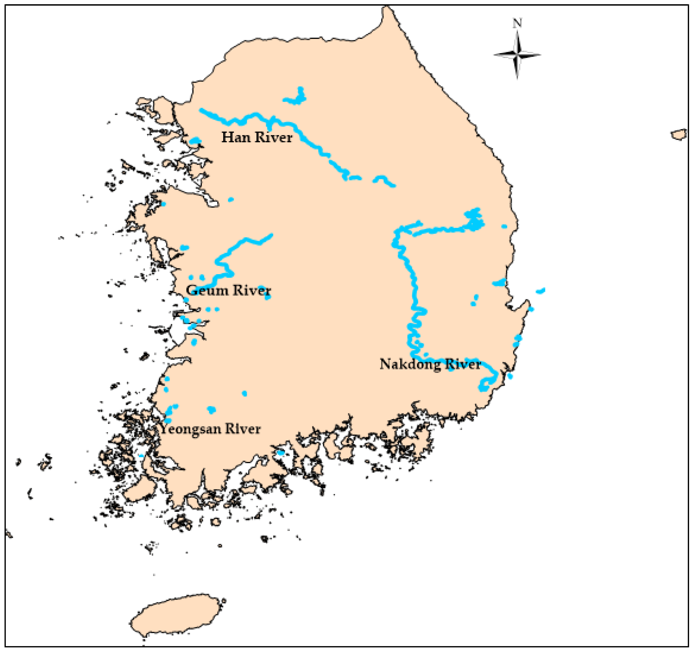
2.1. Study Area
2.2. South Korea’s Net Virtual Water Trade for Grain Crops
2.3. Grain Virtual Water Trade Decomposition
2.4. Tapio Decoupling Elasticity Model
2.5. Data Sources
3. Results
3.1. Net Volume of Grain Virtual Water Trade
3.2. Driving Factors of Net Virtual Water Trade
3.3. Analysis of Decoupling Characteristics of South Korea’s Net Virtual Water Trade
4. Discussion
5. Conclusions
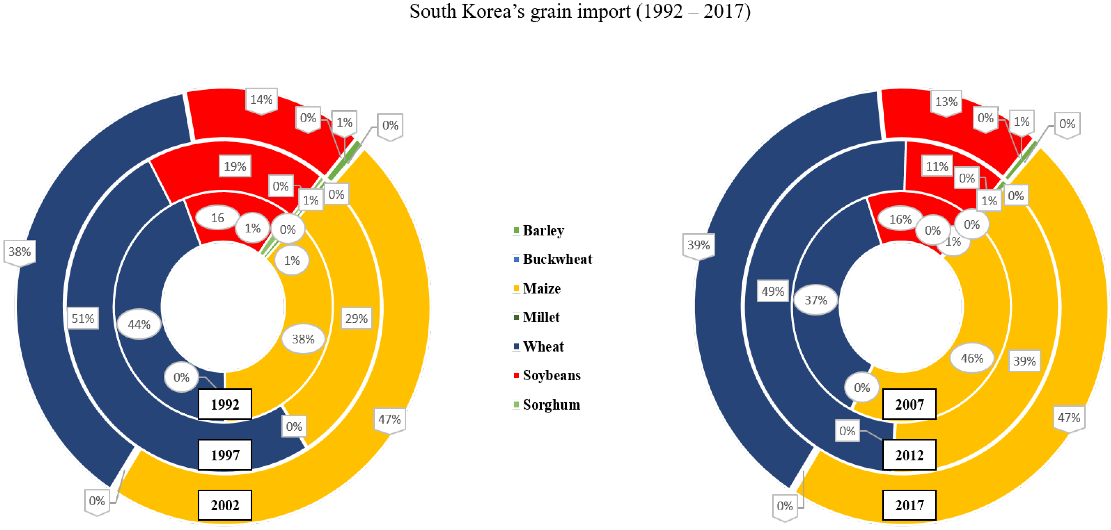
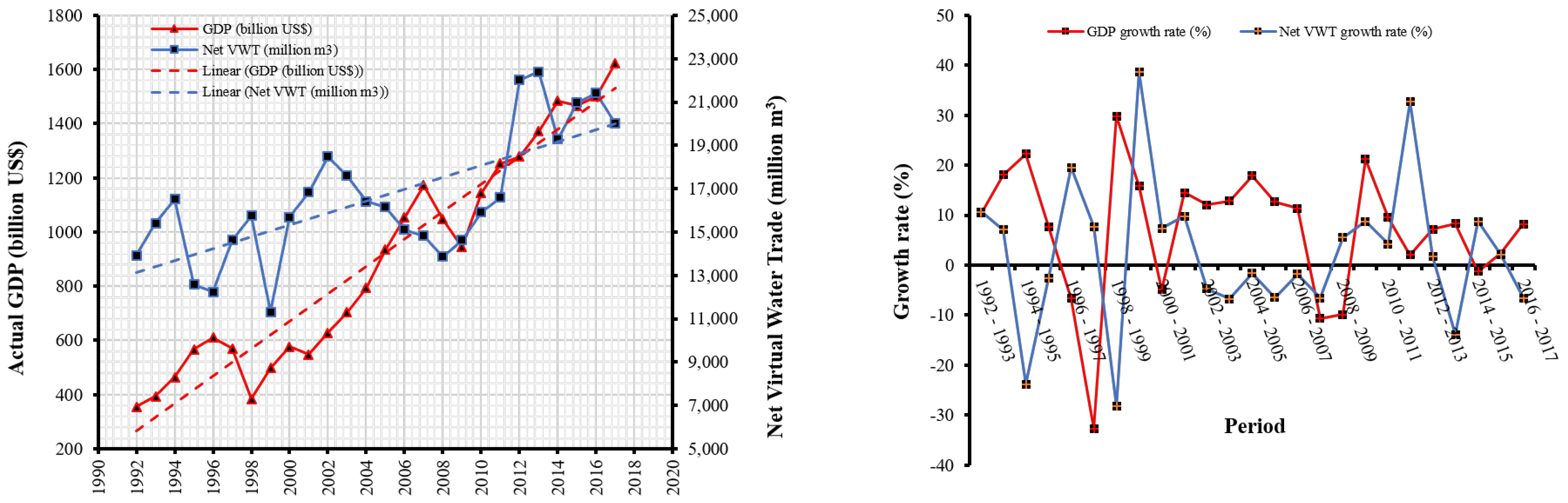
- South Korea was a significant importer of grains (especially maize, wheat, and soybeans). Despite rising trends in both the VWI and the VWE, there was a considerable gap in the volumes of virtual water imported and exported between 1992 and 2017. Population increase and lifestyle changes over the past 50 years have had an impact on the demand and supply of food, as well as the usage of land and water. Understanding these changes is crucial for the management of water resources.
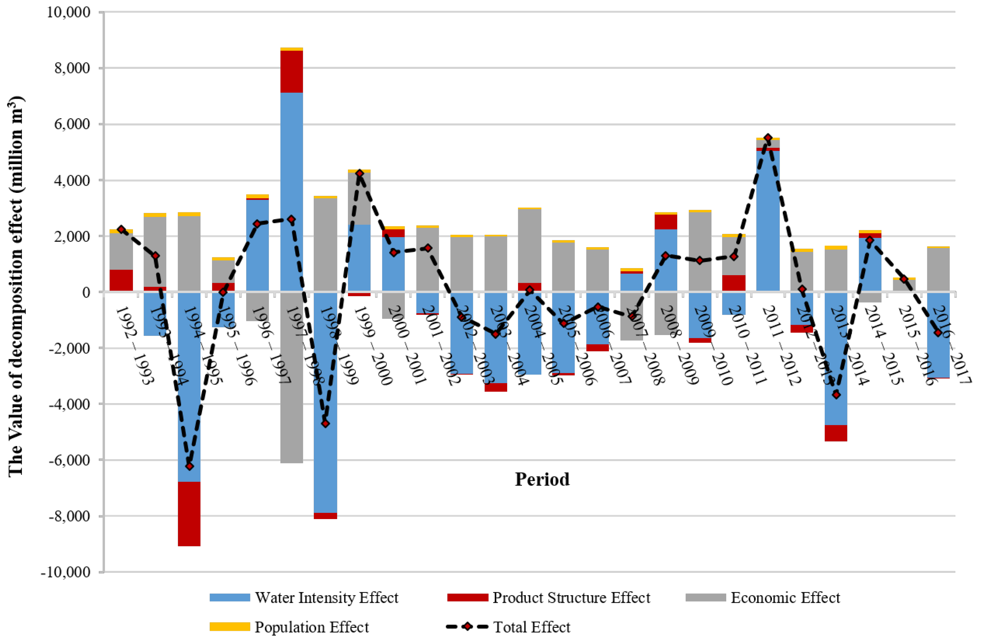
- The most important drivers of net virtual water flows were the economic and water intensity effects. The difference is that whereas the water intensity had a substantial negative impact on net virtual water trade, the economic effect had a positive one. Product structure and population effects, on the other hand, had a smaller impact on the increase in net virtual water trade.
- The decoupling status between water intensity and economic growth was strong decoupling, while product structure and economic growth showed expansive negative decoupling. In addition, the decoupling status between population size and economic growth was mainly weak decoupling for most of the study periods.
Author Contributions
Funding
Institutional Review Board Statement
Informed Consent Statement
Data Availability Statement
Conflicts of Interest
Appendix A

| Year | VWT Change | ||||
|---|---|---|---|---|---|
| Water Intensity Effect | Product Structure Effect | Economic Effect | Population Effect | Total Effect | |
| 1992–1993 | −48.644 | −39.178 | 8.109 | 0.923 | −78.790 |
| 1993–1994 | 3.055 | 1.047 | 12.555 | 0.810 | 17.467 |
| 1994–1995 | −3.495 | 38.405 | 18.417 | 0.973 | 54.300 |
| 1995–1996 | 18.485 | 12.551 | 7.617 | 1.124 | 39.777 |
| 1996–1997 | −57.313 | −57.985 | −7.526 | 0.906 | −121.918 |
| 1997–1998 | 31.057 | 16.852 | −28.173 | 0.504 | 20.240 |
| 1998–1999 | 13.269 | 17.453 | 22.432 | 0.629 | 53.783 |
| 1999–2000 | 5.820 | 36.913 | 16.491 | 0.996 | 60.220 |
| 2000–2001 | 52.508 | 19.398 | −8.910 | 1.170 | 64.165 |
| 2001–2002 | −64.218 | −44.450 | 19.901 | 0.885 | −87.882 |
| 2002–2003 | −33.949 | −16.395 | 13.249 | 0.633 | −36.462 |
| 2003–2004 | −25.305 | −47.203 | 12.425 | 0.420 | −59.662 |
| 2004–2005 | −16.247 | 20.187 | 16.240 | 0.212 | 20.391 |
| 2005–2006 | −69.981 | −52.677 | 7.292 | 0.336 | −115.030 |
| 2006–2007 | 19.328 | 35.215 | 5.025 | 0.248 | 59.815 |
| 2007–2008 | 4.716 | −8.986 | −7.393 | 0.466 | −11.197 |
| 2008–2009 | −26.121 | −26.607 | −4.703 | 0.222 | −57.209 |
| 2009–2010 | 15.122 | 9.352 | 7.479 | 0.199 | 32.152 |
| 2010–2011 | 22.194 | 13.418 | 5.464 | 0.504 | 41.579 |
| 2011–2012 | 58.636 | 60.753 | 1.585 | 0.568 | 121.542 |
| 2012–2013 | −52.069 | −36.159 | 7.701 | 0.538 | −79.990 |
| 2013–2014 | 21.269 | 16.146 | 8.203 | 0.703 | 46.322 |
| 2014–2015 | 0.877 | 13.718 | −2.272 | 0.671 | 12.994 |
| 2015–2016 | −61.702 | −35.511 | 1.806 | 0.373 | −95.034 |
| 2016–2017 | 31.486 | 16.927 | 6.513 | 0.239 | 55.165 |
| Sum | −161.223 | −36.815 | 139.525 | 15.253 | −43.260 |
| Year | VWT Change | ||||
|---|---|---|---|---|---|
| Water Intensity Effect | Product Structure Effect | Economic Effect | Population Effect | Total Effect | |
| 1992–1993 | 1.309 | 1.452 | 0.310 | 0.035 | 3.106 |
| 1993–1994 | −2.373 | −2.389 | 0.528 | 0.034 | −4.200 |
| 1994–1995 | 1.908 | 2.595 | 0.710 | 0.038 | 5.251 |
| 1995–1996 | −3.491 | −3.375 | 0.215 | 0.032 | −6.619 |
| 1996–1997 | 0.271 | 0.154 | −0.158 | 0.019 | 0.287 |
| 1997–1998 | 1.086 | 0.592 | −0.889 | 0.016 | 0.805 |
| 1998–1999 | 0.316 | 0.852 | 0.711 | 0.020 | 1.899 |
| 1999–2000 | 2.131 | 1.805 | 0.640 | 0.039 | 4.615 |
| 2000–2001 | 1.373 | 0.551 | −0.390 | 0.051 | 1.586 |
| 2001–2002 | −0.253 | −0.353 | 0.985 | 0.044 | 0.423 |
| 2002–2003 | −3.735 | −3.479 | 0.689 | 0.033 | −6.492 |
| 2003–2004 | 1.031 | 0.906 | 0.678 | 0.023 | 2.638 |
| 2004–2005 | −0.462 | 2.746 | 1.142 | 0.015 | 3.441 |
| 2005–2006 | −1.277 | 4.759 | 0.818 | 0.038 | 4.338 |
| 2006–2007 | −0.968 | −2.699 | 0.702 | 0.035 | −2.931 |
| 2007–2008 | 0.183 | −2.820 | −0.779 | 0.049 | −3.367 |
| 2008–2009 | −1.440 | 0.414 | −0.561 | 0.026 | −1.561 |
| 2009–2010 | −1.339 | 0.360 | 0.734 | 0.020 | −0.226 |
| 2010–2011 | 0.860 | 0.644 | 0.352 | 0.032 | 1.889 |
| 2011–2012 | −0.999 | −2.383 | 0.065 | 0.023 | −3.294 |
| 2012–2013 | 0.237 | 0.811 | 0.276 | 0.019 | 1.343 |
| 2013–2014 | 0.600 | 1.889 | 0.365 | 0.031 | 2.885 |
| 2014–2015 | −1.348 | 0.385 | −0.085 | 0.025 | −1.023 |
| 2015–2016 | 0.574 | 1.913 | 0.085 | 0.018 | 2.589 |
| 2016–2017 | −0.137 | −2.143 | 0.374 | 0.014 | −1.893 |
| Sum | −5.942 | 3.187 | 7.515 | 0.728 | 5.488 |
| Year | VWT Change | ||||
|---|---|---|---|---|---|
| Water Intensity Effect | Product Structure Effect | Economic Effect | Population Effect | Total Effect | |
| 1992–1993 | −607.030 | −746.528 | 464.521 | 52.897 | −836.140 |
| 1993–1994 | −1299.143 | −499.564 | 767.359 | 49.478 | −981.869 |
| 1994–1995 | −256.183 | 2224.647 | 961.826 | 50.804 | 2981.095 |
| 1995–1996 | −428.308 | −281.407 | 350.284 | 51.675 | −307.756 |
| 1996–1997 | −772.050 | −284.875 | −376.874 | 45.364 | −1388.435 |
| 1997–1998 | 2503.413 | −577.816 | −1869.373 | 33.441 | 89.665 |
| 1998–1999 | −1063.659 | 457.768 | 1295.248 | 36.301 | 725.658 |
| 1999–2000 | 800.433 | 303.732 | 837.121 | 50.565 | 1991.851 |
| 2000–2001 | 1080.774 | −124.054 | −425.479 | 55.856 | 587.098 |
| 2001–2002 | −49.865 | 61.984 | 1059.923 | 47.154 | 1119.195 |
| 2002–2003 | −1583.085 | −372.209 | 908.540 | 43.431 | −1003.322 |
| 2003–2004 | −1475.969 | 690.729 | 913.476 | 30.909 | 159.146 |
| 2004–2005 | −1670.236 | −294.704 | 1184.341 | 15.472 | −765.126 |
| 2005–2006 | −1337.207 | 389.555 | 774.451 | 35.707 | −137.494 |
| 2006–2007 | −446.624 | 336.559 | 682.837 | 33.712 | 606.484 |
| 2007–2008 | −212.841 | −178.111 | −763.606 | 48.087 | −1106.470 |
| 2008–2009 | −63.589 | −625.400 | −605.839 | 28.583 | −1266.244 |
| 2009–2010 | −532.522 | 336.640 | 1029.648 | 27.389 | 861.156 |
| 2010–2011 | −387.143 | −333.444 | 486.940 | 44.876 | −188.771 |
| 2011–2012 | 2548.623 | −131.714 | 105.080 | 37.695 | 2559.684 |
| 2012–2013 | 2080.247 | 438.556 | 646.967 | 45.165 | 3210.935 |
| 2013–2014 | −2439.698 | 657.557 | 773.281 | 66.282 | −942.577 |
| 2014–2015 | 1723.407 | −154.560 | −188.226 | 55.616 | 1436.237 |
| 2015–2016 | −1102.106 | −321.435 | 209.782 | 43.388 | −1170.372 |
| 2016–2017 | −1868.444 | −119.684 | 762.157 | 27.999 | −1197.973 |
| Sum | −6858.805 | 852.223 | 9984.385 | 1057.849 | 5035.652 |
| Year | VWT Change | ||||
|---|---|---|---|---|---|
| Water Intensity Effect | Product Structure Effect | Economic Effect | Population Effect | Total Effect | |
| 1992–1993 | 4.939 | 5.006 | 0.778 | 0.089 | 10.811 |
| 1993–1994 | 2.078 | 3.467 | 2.189 | 0.141 | 7.875 |
| 1994–1995 | −8.213 | −3.920 | 2.552 | 0.135 | −9.446 |
| 1995–1996 | 3.146 | 1.978 | 0.824 | 0.122 | 6.070 |
| 1996–1997 | 4.274 | 5.888 | −1.281 | 0.154 | 9.036 |
| 1997–1998 | 0.716 | −5.192 | −6.152 | 0.110 | −10.518 |
| 1998–1999 | 2.259 | 6.573 | 3.982 | 0.112 | 12.925 |
| 1999–2000 | −1.277 | −0.473 | 2.755 | 0.166 | 1.171 |
| 2000–2001 | 5.814 | 1.642 | −1.343 | 0.176 | 6.289 |
| 2001–2002 | −3.579 | −5.078 | 3.288 | 0.146 | −5.223 |
| 2002–2003 | 4.146 | 7.197 | 3.121 | 0.149 | 14.613 |
| 2003–2004 | 5.646 | 11.059 | 4.394 | 0.149 | 21.248 |
| 2004–2005 | −19.097 | −2.390 | 5.815 | 0.076 | −15.597 |
| 2005–2006 | −7.320 | −2.678 | 3.140 | 0.145 | −6.713 |
| 2006–2007 | 0.380 | −0.392 | 2.785 | 0.138 | 2.910 |
| 2007–2008 | 0.602 | −10.390 | −3.331 | 0.210 | −12.908 |
| 2008–2009 | 2.011 | 8.780 | −2.840 | 0.134 | 8.084 |
| 2009–2010 | −5.890 | 1.477 | 4.712 | 0.125 | 0.424 |
| 2010–2011 | −0.053 | 0.429 | 2.150 | 0.198 | 2.724 |
| 2011–2012 | −2.707 | −7.278 | 0.378 | 0.136 | −9.471 |
| 2012–2013 | 2.635 | 6.324 | 1.756 | 0.123 | 10.837 |
| 2013–2014 | −6.923 | 2.778 | 1.963 | 0.168 | −2.015 |
| 2014–2015 | 5.836 | 1.944 | −0.484 | 0.143 | 7.439 |
| 2015–2016 | −3.035 | 0.579 | 0.552 | 0.114 | −1.790 |
| 2016–2017 | −4.205 | −1.349 | 2.028 | 0.075 | −3.451 |
| Sum | −17.818 | 25.980 | 33.731 | 3.432 | 45.325 |
| Year | VWT Change | ||||
|---|---|---|---|---|---|
| Water Intensity Effect | Product Structure Effect | Economic Effect | Population Effect | Total Effect | |
| 1992–1993 | 1354.596 | 1854.659 | 639.481 | 72.821 | 3921.557 |
| 1993–1994 | −184.664 | 513.094 | 1385.891 | 89.361 | 1803.682 |
| 1994–1995 | −6380.430 | −4526.095 | 1278.909 | 67.553 | −9560.063 |
| 1995–1996 | −816.860 | 720.019 | 274.650 | 40.517 | 218.327 |
| 1996–1997 | 3832.318 | −159.414 | −432.743 | 52.089 | 3292.249 |
| 1997–1998 | 3989.325 | 2385.183 | −3180.983 | 56.905 | 3250.429 |
| 1998–1999 | −6312.979 | −539.804 | 1404.110 | 39.352 | −5409.320 |
| 1999–2000 | 1874.252 | −598.202 | 638.553 | 38.571 | 1953.174 |
| 2000–2001 | 941.557 | 694.489 | −368.831 | 48.420 | 1315.635 |
| 2001–2002 | −543.822 | −188.712 | 885.389 | 39.389 | 192.244 |
| 2002–2003 | −1097.870 | 52.914 | 742.321 | 35.485 | −267.150 |
| 2003–2004 | −1185.003 | −934.053 | 759.655 | 25.704 | −1333.697 |
| 2004–2005 | −925.267 | 847.667 | 1029.912 | 13.455 | 965.766 |
| 2005–2006 | −878.000 | 4.696 | 722.739 | 33.323 | −117.242 |
| 2006–2007 | −1402.439 | −493.017 | 602.813 | 29.762 | −1262.881 |
| 2007–2008 | 206.751 | −170.006 | −640.837 | 40.356 | −563.736 |
| 2008–2009 | 2563.848 | 823.124 | −658.564 | 31.071 | 2759.480 |
| 2009–2010 | −723.538 | −124.431 | 1386.186 | 36.873 | 575.091 |
| 2010–2011 | −213.655 | 1199.589 | 668.491 | 61.608 | 1716.032 |
| 2011–2012 | 2436.285 | 135.460 | 139.596 | 50.076 | 2761.417 |
| 2012–2013 | −2883.803 | −748.426 | 636.141 | 44.409 | −2951.679 |
| 2013–2014 | −2472.775 | −1622.239 | 566.428 | 48.552 | −3480.035 |
| 2014–2015 | 93.458 | 459.425 | −122.087 | 36.073 | 466.869 |
| 2015–2016 | 1161.917 | 242.855 | 143.775 | 29.736 | 1578.283 |
| 2016–2017 | −946.935 | −27.282 | 613.704 | 22.545 | −337.968 |
| Sum | −8513.733 | −198.505 | 9114.700 | 1084.006 | 1486.468 |
| Year | VWT Change | ||||
|---|---|---|---|---|---|
| Water Intensity Effect | Product Structure Effect | Economic Effect | Population Effect | Total Effect | |
| 1992–1993 | −519.141 | −172.572 | 179.990 | 20.496 | −491.227 |
| 1993–1994 | −40.499 | 197.230 | 312.919 | 20.177 | 489.826 |
| 1994–1995 | −163.546 | −53.209 | 438.308 | 23.152 | 244.705 |
| 1995–1996 | −150.758 | −259.497 | 159.471 | 23.526 | −227.258 |
| 1996–1997 | 395.669 | 655.005 | −201.987 | 24.313 | 872.999 |
| 1997–1998 | 669.507 | −284.496 | −1021.950 | 18.282 | −618.657 |
| 1998–1999 | −520.108 | −186.076 | 614.957 | 17.235 | −73.992 |
| 1999–2000 | −270.094 | 122.014 | 350.468 | 21.169 | 223.557 |
| 2000–2001 | −108.479 | −331.901 | −144.013 | 18.906 | −565.487 |
| 2001–2002 | −88.247 | 104.702 | 320.968 | 14.279 | 351.702 |
| 2002–2003 | −206.297 | 311.265 | 286.564 | 13.699 | 405.230 |
| 2003–2004 | −683.783 | −94.853 | 292.173 | 9.886 | −476.577 |
| 2004–2005 | −175.520 | −190.923 | 392.337 | 5.125 | 31.019 |
| 2005–2006 | −608.297 | −429.896 | 269.205 | 12.412 | −756.577 |
| 2006–2007 | −48.873 | −142.459 | 235.512 | 11.627 | 55.808 |
| 2007–2008 | 656.322 | 474.829 | −311.095 | 19.591 | 839.647 |
| 2008–2009 | −232.660 | 351.712 | −274.016 | 12.928 | −142.035 |
| 2009–2010 | −403.057 | −377.530 | 429.247 | 11.418 | −339.921 |
| 2010–2011 | −227.085 | −276.939 | 192.076 | 17.702 | −294.246 |
| 2011–2012 | 2.115 | 44.161 | 33.961 | 12.183 | 92.421 |
| 2012–2013 | −316.290 | 57.008 | 147.461 | 10.294 | −101.526 |
| 2013–2014 | 136.035 | 378.471 | 171.518 | 14.702 | 700.727 |
| 2014–2015 | 123.230 | −162.048 | −45.517 | 13.449 | −70.886 |
| 2015–2016 | −38.167 | 133.108 | 50.034 | 10.348 | 155.323 |
| 2016–2017 | −265.473 | 103.037 | 197.972 | 7.273 | 42.808 |
| Sum | −3083.497 | −29.856 | 3076.562 | 384.172 | 347.381 |
| Year | VWT Change | ||||
|---|---|---|---|---|---|
| Water Intensity Effect | Product Structure Effect | Economic Effect | Population Effect | Total Effect | |
| 1992–1993 | −148.371 | −144.888 | 9.025 | 1.028 | −283.207 |
| 1993–1994 | −30.994 | −23.221 | 5.134 | 0.331 | −48.749 |
| 1994–1995 | 23.557 | 25.320 | 6.637 | 0.351 | 55.865 |
| 1995–1996 | 124.585 | 129.931 | 6.778 | 1.000 | 262.293 |
| 1996–1997 | −110.068 | −98.292 | −9.023 | 1.086 | −216.297 |
| 1997–1998 | −57.064 | −53.871 | −7.589 | 0.136 | −118.388 |
| 1998–1999 | 1.656 | 2.539 | 0.824 | 0.023 | 5.043 |
| 1999–2000 | −1.854 | −1.501 | 0.553 | 0.033 | −2.769 |
| 2000–2001 | 0.958 | 0.087 | −0.220 | 0.029 | 0.854 |
| 2001–2002 | −0.484 | 0.099 | 0.546 | 0.024 | 0.185 |
| 2002–2003 | −0.123 | −0.186 | 0.481 | 0.023 | 0.194 |
| 2003–2004 | 119.718 | 60.198 | 4.374 | 0.148 | 184.438 |
| 2004–2005 | −130.400 | −45.013 | 6.050 | 0.079 | −169.284 |
| 2005–2006 | −1.252 | −1.217 | 0.480 | 0.022 | −1.967 |
| 2006–2007 | 8.863 | 7.450 | 0.788 | 0.039 | 17.140 |
| 2007–2008 | −9.313 | −9.809 | −0.884 | 0.056 | −19.951 |
| 2008–2009 | 0.993 | 2.470 | −0.403 | 0.019 | 3.079 |
| 2009–2010 | −0.931 | 0.004 | 0.733 | 0.020 | −0.174 |
| 2010–2011 | 1.256 | 1.171 | 0.385 | 0.035 | 2.848 |
| 2011–2012 | −0.297 | −0.416 | 0.079 | 0.028 | −0.605 |
| 2012–2013 | 0.139 | 0.407 | 0.363 | 0.025 | 0.936 |
| 2013–2014 | −1.316 | −1.582 | 0.395 | 0.034 | −2.469 |
| 2014–2015 | −0.385 | −0.122 | −0.084 | 0.025 | −0.566 |
| 2015–2016 | −0.113 | 0.322 | 0.086 | 0.018 | 0.314 |
| 2016–2017 | −1.167 | 0.091 | 0.311 | 0.011 | −0.754 |
| Sum | −212.405 | −150.030 | 25.821 | 4.623 | −331.991 |
References
- Kong, Y.; He, W.; Yuan, L.; Shen, J.; An, M.; Degefu, D.M.; Gao, X.; Zhang, Z.; Sun, F.; Wan, Z. Decoupling analysis of water footprint and economic growth: A case study of Beijing–Tianjin–Hebei Region from 2004 to 2017. Int. J. Environ. Res. Public Health 2019, 16, 4873. [Google Scholar] [CrossRef] [Green Version]
- Chen, X.; Zhao, B.; Shuai, C.; Qu, S.; Xu, M. Global spread of water scarcity risk through trade. Resour. Conserv. Recycl. 2022, 187, 106643. [Google Scholar] [CrossRef]
- Gleick, P.H.; Cooley, H. Freshwater Scarcity. Annu. Rev. Environ. Resour. 2021, 46, 319–348. [Google Scholar] [CrossRef]
- Rosa, L.; Chiarelli, D.D.; Rulli, M.C.; Dell’Angelo, J.; D’Odorico, P. Global agricultural economic water scarcity. Sci. Adv. 2020, 6, eaaz6031. [Google Scholar] [CrossRef]
- Mekonnen, M.M.; Hoekstra, A.Y. Four billion people facing severe water scarcity. Sci. Adv. 2016, 2, e1500323. [Google Scholar] [CrossRef] [Green Version]
- McLennan, M. The Global Risks Report 2021, 16th ed.; World Economic Forum: Cologny, Switzerland, 2021. [Google Scholar]
- Qin, Y.; Mueller, N.D.; Siebert, S.; Jackson, R.B.; AghaKouchak, A.; Zimmerman, J.B.; Tong, D.; Hong, C.; Davis, S.J. Flexibility and intensity of global water use. Nat. Sustain. 2019, 2, 515–523. [Google Scholar] [CrossRef]
- Richter, B.D.; Bartak, D.; Caldwell, P.; Davis, K.F.; Debaere, P.; Hoekstra, A.Y.; Li, T.; Marston, L.; McManamay, R.; Mekonnen, M.M. Water scarcity and fish imperilment driven by beef production. Nat. Sustain. 2020, 3, 319–328. [Google Scholar] [CrossRef]
- Adelodun, B.; Odey, G.; Cho, H.; Lee, S.; Adeyemi, K.A.; Choi, K.S. Spatial-temporal variability of climate indices in Chungcheong provinces of Korea: Application of graphical innovative methods for trend analysis. Atmos. Res. 2022, 280, 106420. [Google Scholar] [CrossRef]
- Degefu, D.M.; He, W.; Yuan, L.; Zhao, J.H. Water allocation in transboundary river basins under water scarcity: A cooperative bargaining approach. Water Resour. Manag. 2016, 30, 4451–4466. [Google Scholar] [CrossRef]
- Ge, L.; Xie, G.; Zhang, C.; Li, S.; Qi, Y.; Cao, S.; He, T. An evaluation of China’s water footprint. Water Resour. Manag. 2011, 25, 2633–2647. [Google Scholar] [CrossRef]
- Qu, S.; Liang, S.; Konar, M.; Zhu, Z.; Chiu, A.S.; Jia, X.; Xu, M. Virtual water scarcity risk to the global trade system. Environ. Sci. Technol. 2018, 52, 673–683. [Google Scholar] [CrossRef] [PubMed]
- Distefano, T.; Isaza, A.S.; Muñoz, E.; Builes, T. Sub-national water–food–labour nexus in Colombia. J. Clean. Prod. 2022, 335, 130138. [Google Scholar] [CrossRef]
- Wang, N.; Choi, Y. Challenges for sustainable water use in the urban industry of Korea based on the global non-radial directional distance function model. Sustainability 2019, 11, 3895. [Google Scholar] [CrossRef] [Green Version]
- Choi, I.-C.; Shin, H.-J.; Nguyen, T.T.; Tenhunen, J. Water policy reforms in South Korea: A historical review and ongoing challenges for sustainable water governance and management. Water 2017, 9, 717. [Google Scholar] [CrossRef] [Green Version]
- Cho, C.-J. The Korean growth-management programs: Issues, problems and possible reforms. Land Use Policy 2002, 19, 13–27. [Google Scholar] [CrossRef]
- Sun, J.; Yin, Y.; Sun, S.; Wang, Y.; Yu, X.; Yan, K. Review on research status of virtual water: The perspective of accounting methods, impact assessment and limitations. Agric. Water Manag. 2021, 243, 106407. [Google Scholar] [CrossRef]
- Hoekstra, A.Y.; Hung, P.Q. Virtual water trade. In Proceedings of the International Expert Meeting on Virtual Water Trade, Delft, The Netherlands, 12–13 December 2003; pp. 1–244. [Google Scholar]
- Konar, M.; Dalin, C.; Hanasaki, N.; Rinaldo, A.; Rodriguez-Iturbe, I. Temporal dynamics of blue and green virtual water trade networks. Water Resour. Res. 2012, 48, W07509. [Google Scholar] [CrossRef]
- Matveeva, L.G.; Chernova, O.G.A.; Kosolapova, N.Y.A.; Kosolapov, A.E. Assessment of water resources use efficiency based on the Russian Federation’s gross regional product water intensity indicator. Reg. Stat. 2018, 8, 154–169. [Google Scholar] [CrossRef]
- Hsieh, J.C.; Ma, L.H.; Chiu, Y.H. Assessing China’s use efficiency of water resources from the resampling super data envelopment analysis approach. Water 2019, 11, 1069. [Google Scholar] [CrossRef] [Green Version]
- Kim, S. LMDI decomposition analysis of energy consumption in the Korean manufacturing sector. Sustainability 2017, 9, 202. [Google Scholar] [CrossRef]
- Fan, W.; Meng, M.; Lu, J.; Dong, X.; Wei, H.; Wang, X.; Zhang, Q. Decoupling elasticity and driving factors of energy consumption and economic development in the Qinghai-Tibet Plateau. Sustainability 2020, 12, 1326. [Google Scholar] [CrossRef] [Green Version]
- Khan, S.; Majeed, M.T. Drivers of decoupling economic growth from carbon emission: Empirical analysis of ASEAN countries using decoupling and decomposition model. Pak. J. Commer. Soc. Sci. 2020, 14, 450–483. [Google Scholar]
- Ang, B.W. Decomposition analysis for policymaking in energy: Which is the preferred method? Energy Policy 2004, 32, 1131–1139. [Google Scholar] [CrossRef]
- Qian, Y.; Tian, X.; Geng, Y.; Zhong, S.; Cui, X.; Zhang, X.; Moss, D.A.; Bleischwitz, R. Driving factors of agricultural virtual water trade between China and the belt and road countries. Environ. Sci. Technol. 2019, 53, 5877–5886. [Google Scholar] [CrossRef]
- Gao, C.; Xie, R.; Zhang, Y.; Zhu, K. Drivers of dynamic evolution in provincial production water usage: Perspective of regional relevance. Environ. Sci. Pollut. Res. 2021, 28, 15130–15146. [Google Scholar] [CrossRef] [PubMed]
- Song, J.; Yin, Y.; Xu, H.; Wang, Y.; Wu, P.; Sun, S. Drivers of domestic grain virtual water flow: A study for China. Agric. Water Manag. 2020, 239, 106175. [Google Scholar] [CrossRef]
- Han, S.-Y.; Kwak, S.J.; Yoo, S.H. Valuing environmental impacts of large dam construction in Korea: An application of choice experiments. Environ. Impact Assess. Rev. 2008, 28, 256–266. [Google Scholar] [CrossRef]
- Enevoldsen, M.K.; Ryelund, A.V.; Andersen, M.S. Decoupling of industrial energy consumption and CO2-emissions in energy-intensive industries in Scandinavia. Energy Econ. 2007, 29, 665–692. [Google Scholar] [CrossRef]
- Tapio, P. Towards a theory of decoupling: Degrees of decoupling in the EU and the case of road traffic in Finland between 1970 and 2001. Transp. Policy 2005, 12, 137–151. [Google Scholar] [CrossRef] [Green Version]
- Wu, D.; Yuan, C.; Liu, H. The decoupling states of CO2 emissions in the Chinese transport sector from 1994 to 2012: A perspective on fuel types. Energy Environ. 2018, 29, 591–612. [Google Scholar] [CrossRef]
- Yu, Z.; Qingshan, Y. Decoupling agricultural water consumption and environmental impact from crop production based on the water footprint method: A case study for the Heilongjiang land reclamation area, China. Ecol. Indic. 2014, 43, 29–35. [Google Scholar] [CrossRef]
- Wang, Q.; Jiang, R.; Li, R. Decoupling analysis of economic growth from water use in City: A case study of Beijing, Shanghai, and Guangzhou of China. Sustain. Cities Soc. 2018, 41, 86–94. [Google Scholar] [CrossRef]
- Park, S.; Lee, M.; Park, K.; An, Y. Calculating virtual water for international water transactions: Deriving water footprints in South Korea. J. Korea Water Resour. Assoc. 2020, 53, 765–772. [Google Scholar]
- Lee, S.H.; Yoo, S.H.; Choi, J.Y.; Shin, A. Evaluation of the dependency and intensity of the virtual water trade in Korea. Irrig. Drain. 2016, 65, 48–56. [Google Scholar] [CrossRef]
- Odey, G.; Adelodun, B.; Cho, G.; Lee, S.; Adeyemi, K.A.; Choi, K.S. Modeling the Influence of Seasonal Climate Variability on Soybean Yield in a Temperate Environment: South Korea as a Case Study. Int. J. Plant Prod. 2022, 16, 209–222. [Google Scholar] [CrossRef]
- Min, K.-J. The Role of the State and the Market in the Korean Water Sector: Strategic Decision Making Approach for Good Governance. Ph.D. Thesis, University of Bath, Claverton Down, UK, 2011. [Google Scholar]
- Ministry of Land, Infrastructure and Transportation of Korea (MOLIT); Korea Water Resources Corporation (K-Water). Water for the Future: Water and Sustainable Development; K-Water: Daejeon, Republic of Korea, 2015. [Google Scholar]
- Kim, K.M. Improvement of the Han River Watershed Management Fund Policies; National Assembly Research Service (NARS) Issue Report 160; NARS: Seoul, Republic of Korea, 2012. [Google Scholar]
- Yoo, S.H.; Lee, S.H.; Choi, J.Y.; Im, J.B. Estimation of potential water requirements using water footprint for the target of food self-sufficiency in South Korea. Paddy Water Environ. 2016, 14, 259–269. [Google Scholar] [CrossRef]
- Shivaswamy, G.; Kallega, H.K.; Anuja, A.; Singh, K. An assessment of India’s virtual water trade in major food products. Agric. Econ. Res. Rev. 2021, 34, 133–141. [Google Scholar] [CrossRef]
- FAO. Crops and Livestock Products; FAO: Rome, Italy, 2022; Available online: http://www.fao.org/faostat/en/#data/QCL (accessed on 7 September 2022).
- Yoo, S.H.; Lee, S.H.; Choi, J.Y. Estimation of water footprint for upland crop production in Korea. J. Korean Soc. Agric. Eng. 2014, 56, 65–74. [Google Scholar]
- Mekonnen, M.M.; Hoekstra, A.Y. The green, blue and grey water footprint of crops and derived crop products. Hydrol. Earth Syst. Sci. 2011, 15, 1577–1600. [Google Scholar] [CrossRef] [Green Version]
- World-Bank. GDP (Current US$)–Korea, Rep. Available online: https://data.worldbank.org/indicator/NY.GDP.MKTP.CD?locations=KR (accessed on 7 September 2022).
- De Fraiture, C.; Cai, X.; Amarasinghe, U.; Rosegrant, M.; Molden, D. Does International Cereal Trade Save Water? The Impact of Virtual Water Trade on Global Water Use; Iwmi: Colombo, Sri Lanka, 2004; Volume 4. [Google Scholar]
- Hoekstra, A.Y.; Mekonnen, M.M. The water footprint of humanity. Proc. Natl. Acad. Sci. USA 2012, 109, 3232–3237. [Google Scholar] [CrossRef] [Green Version]
- IPCC, I.P.o.C.C. Climate Change Impacts, Adaption and Vulnerability; Cambridge University Press: Cambridge, UK, 2007. [Google Scholar]
- Chouchane, H.; Krol, M.S.; Hoekstra, A.Y. Virtual water trade patterns in relation to environmental and socioeconomic factors: A case study for Tunisia. Sci. Total Environ. 2018, 613, 287–297. [Google Scholar] [CrossRef] [PubMed] [Green Version]
- Xia, W.; Chen, X.; Song, C.; Pérez-Carrera, A. Driving factors of virtual water in international grain trade: A study for belt and road countries. Agric. Water Manag. 2022, 262, 107441. [Google Scholar] [CrossRef]
- Lee, S.; Jung, K.Y.; Chun, H.C.; Choi, Y.D.; Kang, H.W. Response of soybean (Glycine max L.) to subsurface drip irrigation with different dripline placements at a sandy-loam soil. Korean J. Soil Sci. Fertil. 2018, 51, 79–89. [Google Scholar] [CrossRef]
- Lee, S.-G.; Adelodun, B.; Ahmad, M.J.; Choi, K.S. Multi-Level Prioritization Analysis of Water Governance Components to Improve Agricultural Water-Saving Policy: A Case Study from Korea. Sustainability 2022, 14, 3248. [Google Scholar] [CrossRef]
- Wang, F.; Cai, B.; Hu, X.; Liu, Y.; Zhang, W. Exploring solutions to alleviate the regional water stress from virtual water flows in China. Sci. Total Environ. 2021, 796, 148971. [Google Scholar] [CrossRef] [PubMed]
- Chae, S.; Lee, J. Smart Decentralized Water Systems in South Korea. In Resilient Water Management Strategies in Urban Settings; Springer: Berlin/Heidelberg, Germany, 2022; pp. 31–46. [Google Scholar]

| Study | Study Period | Type of Study | Variables Utilized |
|---|---|---|---|
| [1] | 2004–2017 | Regional |
|
| [26] | 2000–2016 | Cross-Country |
|
| [28] | 1997–2015 | National |
|
| [27] | 2002–2012 | Regional |
|
| Current study | 1992–2017 | National |
|
| Decoupling Category | Decoupling State | ΔX/X | ΔGDP/GDP | Elasticity Coefficient | Interpretation |
|---|---|---|---|---|---|
| Negative coupling | Expansive negative decoupling (END) | >0 | >0 | (1.2, +∞) | The increasing pace of driving factor (X) is largely greater than that of economic growth (GDP). |
| Strong negative decoupling (SND) | >0 | <0 | (−∞, 0) | Driving factor (X) increases while economic growth (GDP) decreases. | |
| Weak negative decoupling (WND) | <0 | <0 | (0, 0.8) | The decreasing pace of driving factor (X) is largely smaller than that of economic growth (GDP). | |
| Coupling | Expansive coupling (EC) | >0 | >0 | (0.8, 1.2) | The increasing pace of driving factor (X) is relatively equal to that of economic growth (GDP). |
| Recessive coupling (RC) | <0 | <0 | (0.8, 1.2) | The decreasing pace of driving factor (X) is relatively equal to that of economic growth (GDP). | |
| Decoupling | Weak decoupling (WD) | >0 | >0 | (0, 0.8) | The increasing pace of driving factor (X) is less than that of economic growth (GDP). |
| Strong decoupling (SD) | <0 | >0 | (−∞, 0) | Driving factor (X) decreases while economic growth (GDP) increases. | |
| Recessive decoupling (RD) | <0 | <0 | (1.2, +∞) | The decreasing pace of driving factor (X) is largely greater than that of economic growth (GDP). |
| Input | Sources |
|---|---|
| Net virtual water trade | Author estimation |
| Gross domestic product (GDP) | [46] |
| Population | [43] |
| Trade matrix | [43] |
| Water footprint | [44,45] |
| Year | Virtual Water Import | Virtual Water Export | Net Virtual Water Trade |
|---|---|---|---|
| 1992 | 13,925.24 | 0.33 | 13,924.91 |
| 1993 | 15,413.20 | 0.13 | 15,413.07 |
| 1994 | 16,507.76 | 0.32 | 16,507.44 |
| 1995 | 12,571.87 | 0.47 | 12,571.40 |
| 1996 | 12,239.55 | 3.52 | 12,236.04 |
| 1997 | 14,625.68 | 2.20 | 14,623.48 |
| 1998 | 15,756.42 | 0.62 | 15,755.80 |
| 1999 | 11,314.77 | 2.28 | 11,312.49 |
| 2000 | 15,684.22 | 4.20 | 15,680.02 |
| 2001 | 16,831.42 | 1.47 | 16,829.95 |
| 2002 | 18,473.55 | 1.15 | 18,472.40 |
| 2003 | 17,602.09 | 2.19 | 17,599.91 |
| 2004 | 16,413.20 | 2.54 | 16,410.66 |
| 2005 | 16,145.58 | 1.88 | 16,143.70 |
| 2006 | 15,101.36 | 0.89 | 15,100.47 |
| 2007 | 14,836.71 | 0.55 | 14,836.16 |
| 2008 | 13,864.38 | 0.91 | 13,863.47 |
| 2009 | 14,633.26 | 0.69 | 14,632.57 |
| 2010 | 15,916.62 | 1.43 | 15,915.20 |
| 2011 | 16,593.53 | 1.15 | 16,592.39 |
| 2012 | 22,016.46 | 0.97 | 22,015.50 |
| 2013 | 22,393.93 | 6.10 | 22,387.83 |
| 2014 | 19,279.16 | 1.51 | 19,277.65 |
| 2015 | 20,971.18 | 1.21 | 20,969.97 |
| 2016 | 21,420.94 | 3.48 | 21,417.45 |
| 2017 | 20,008.23 | 4.44 | 20,003.79 |
| Average | 16,559.24 | 1.79 | 16,557.45 |
| Year | VWT Change | ||||
|---|---|---|---|---|---|
| Water Intensity Effect | Product Structure Effect | Economic Effect | Population Effect | Total Effect | |
| 1992–1993 | 37.658 | 757.951 | 1302.214 | 148.289 | 2246.112 |
| 1993–1994 | −1552.541 | 189.664 | 2486.576 | 160.331 | 1284.031 |
| 1994–1995 | −6786.401 | −2292.256 | 2707.359 | 143.005 | −6228.293 |
| 1995–1996 | −1253.201 | 320.200 | 799.839 | 117.995 | −15.167 |
| 1996–1997 | 3293.102 | 60.481 | −1029.592 | 123.931 | 2447.921 |
| 1997–1998 | 7138.040 | 1481.252 | −6115.109 | 109.393 | 2613.576 |
| 1998–1999 | −7879.245 | −240.695 | 3342.263 | 93.672 | −4684.004 |
| 1999–2000 | 2409.411 | −135.712 | 1846.581 | 111.539 | 4231.819 |
| 2000–2001 | 1974.505 | 260.213 | −949.186 | 124.608 | 1410.140 |
| 2001–2002 | −750.469 | −71.808 | 2290.999 | 101.922 | 1570.645 |
| 2002–2003 | −2920.913 | −20.894 | 1954.964 | 93.454 | −893.389 |
| 2003–2004 | −3243.665 | −313.216 | 1987.176 | 67.240 | −1502.465 |
| 2004–2005 | −2937.230 | 337.569 | 2635.837 | 34.435 | 70.611 |
| 2005–2006 | −2903.335 | −87.458 | 1778.125 | 81.982 | −1130.686 |
| 2006–2007 | −1870.335 | −259.344 | 1530.462 | 75.561 | −523.656 |
| 2007–2008 | 646.421 | 94.707 | −1727.925 | 108.815 | −877.983 |
| 2008–2009 | 2243.042 | 534.493 | −1546.925 | 72.983 | 1303.593 |
| 2009–2010 | −1652.154 | −154.128 | 2858.739 | 76.044 | 1128.501 |
| 2010–2011 | −803.625 | 604.868 | 1355.859 | 124.955 | 1282.056 |
| 2011–2012 | 5041.655 | 98.584 | 280.744 | 100.710 | 5521.693 |
| 2012–2013 | −1168.903 | −281.479 | 1440.665 | 100.573 | 90.856 |
| 2013–2014 | −4762.808 | −566.980 | 1522.153 | 130.472 | −3677.162 |
| 2014–2015 | 1945.075 | 158.742 | −358.755 | 106.003 | 1851.065 |
| 2015–2016 | −42.631 | 21.831 | 406.119 | 83.995 | 469.314 |
| 2016–2017 | −3054.876 | −30.403 | 1583.058 | 58.156 | −1444.065 |
| Sum | −18,853.423 | 466.184 | 22,382.239 | 2550.063 | 6545.063 |
| Year | Decoupling Elasticity of Water Intensity and GDP | Decoupling Status | Decoupling Elasticity of Product Structure and GDP | Decoupling Status | Decoupling Elasticity of Population Size and GDP | Decoupling Status |
|---|---|---|---|---|---|---|
| 1992–1993 | −0.88891 | Strong decoupling | 2.51624 | END | 0.68413 | Weak decoupling |
| 1993–1994 | −6.57933 | Strong decoupling | −3.61510 | Strong decoupling | 0.39174 | Weak decoupling |
| 1994–1995 | 1.84306 | END | 10.57744 | END | 0.31876 | Weak decoupling |
| 1995–1996 | 22.97925 | END | 27.63861 | END | 0.87111 | Expansive coupling |
| 1996–1997 | −5.88652 | Strong decoupling | 4.70734 | END | −0.99574 | Strong decoupling |
| 1997–1998 | −6.02349 | Strong decoupling | 1.59051 | END | −0.15499 | Strong decoupling |
| 1998–1999 | 0.13148 | Weak decoupling | 7.40025 | END | 0.16763 | Weak decoupling |
| 1999–2000 | 4.70536 | END | 3.05760 | END | 0.37174 | Weak decoupling |
| 2000–2001 | −30.20644 | Strong decoupling | −5.91180 | Strong decoupling | −1.08908 | Strong decoupling |
| 2001–2002 | −5.04942 | Strong decoupling | −2.97002 | Strong decoupling | 0.27919 | Weak decoupling |
| 2002–2003 | −7.93676 | Strong decoupling | −1.78655 | Strong decoupling | 0.30234 | Weak decoupling |
| 2003–2004 | 180.50964 | END | 31.74504 | END | 0.21594 | Weak decoupling |
| 2004–2005 | −11.22938 | Strong decoupling | −0.21111 | Strong decoupling | 0.08314 | Weak decoupling |
| 2005–2006 | −14.64117 | Strong decoupling | −0.56057 | Strong decoupling | 0.29126 | Weak decoupling |
| 2006–2007 | 19.64819 | END | 19.85681 | END | 0.31276 | Weak decoupling |
| 2007–2008 | 2.73515 | END | 13.08692 | END | −0.49941 | Strong decoupling |
| 2008–2009 | −1.21090 | Strong decoupling | −11.81615 | Strong decoupling | −0.36588 | Strong decoupling |
| 2009–2010 | −2.81176 | Strong decoupling | 1.49066 | END | 0.16491 | Weak decoupling |
| 2010–2011 | 7.92047 | END | 7.23773 | END | 0.56635 | Weak decoupling |
| 2011–2012 | 53.85485 | END | 1.58460 | END | 1.83459 | END |
| 2012–2013 | −4.48177 | Strong decoupling | 3.94634 | END | 0.44204 | Weak decoupling |
| 2013–2014 | −6.37136 | Strong decoupling | 6.30188 | END | 0.53262 | Weak decoupling |
| 2014–2015 | −13.04215 | Strong decoupling | −19.22974 | Strong decoupling | −2.96206 | Strong decoupling |
| 2015–2016 | −17.48505 | Strong decoupling | 16.15569 | END | 1.18816 | Expansive coupling |
| 2016–2017 | −4.31514 | Strong decoupling | −1.65950 | Strong decoupling | 0.23867 | Weak decoupling |
Publisher’s Note: MDPI stays neutral with regard to jurisdictional claims in published maps and institutional affiliations. |
© 2022 by the authors. Licensee MDPI, Basel, Switzerland. This article is an open access article distributed under the terms and conditions of the Creative Commons Attribution (CC BY) license (https://creativecommons.org/licenses/by/4.0/).
Share and Cite
Odey, G.; Adelodun, B.; Lee, S.; Adeyemi, K.A.; Cho, G.; Choi, K.S. Environmental and Socioeconomic Determinants of Virtual Water Trade of Grain Products: An Empirical Analysis of South Korea Using Decomposition and Decoupling Model. Agronomy 2022, 12, 3105. https://doi.org/10.3390/agronomy12123105
Odey G, Adelodun B, Lee S, Adeyemi KA, Cho G, Choi KS. Environmental and Socioeconomic Determinants of Virtual Water Trade of Grain Products: An Empirical Analysis of South Korea Using Decomposition and Decoupling Model. Agronomy. 2022; 12(12):3105. https://doi.org/10.3390/agronomy12123105
Chicago/Turabian StyleOdey, Golden, Bashir Adelodun, Seulgi Lee, Khalid Adeola Adeyemi, Gunho Cho, and Kyung Sook Choi. 2022. "Environmental and Socioeconomic Determinants of Virtual Water Trade of Grain Products: An Empirical Analysis of South Korea Using Decomposition and Decoupling Model" Agronomy 12, no. 12: 3105. https://doi.org/10.3390/agronomy12123105