Article

The Hitchhiker’s Guide to Adaptive Dynamics

1
Department of Information and Computer Sciences, Nara Women's University, Kita-Uoya Nishimachi, Nara 630-8506, Japan
2
Department of Mathematics and Mathematical Statistics, Umeå University, 901 87 Umeå, Sweden
3
Evolution and Ecology Program, International Institute for Applied Systems Analysis, Schlossplatz 1, Laxenburg 2361, Austria
4
Department of Biology, Theoretical Population Ecology and Evolution Group, Ecology Bldg., Lund University, 223 62 Lund, Sweden
5
Arbeitsgruppe für nichtlineare Dynamik am Institut für Physik, University of Potsdam, Germany
*
Author to whom correspondence should be addressed.
Games 2013, 4(3), 304-328; https://doi.org/10.3390/g4030304
Submission received: 7 April 2013 / Revised: 9 June 2013 / Accepted: 11 June 2013 / Published: 24 June 2013
(This article belongs to the Special Issue Advances in Evolutionary Game Theory and Applications)

Abstract

:
Adaptive dynamics is a mathematical framework for studying evolution. It extends evolutionary game theory to account for more realistic ecological dynamics and it can incorporate both frequency- and density-dependent selection. This is a practical guide to adaptive dynamics that aims to illustrate how the methodology can be applied to the study of specific systems. The theory is presented in detail for a single, monomorphic, asexually reproducing population. We explain the necessary terminology to understand the basic arguments in models based on adaptive dynamics, including invasion fitness, the selection gradient, pairwise invasibility plots (PIP), evolutionarily singular strategies, and the canonical equation. The presentation is supported with a worked-out example of evolution of arrival times in migratory birds. We show how the adaptive dynamics methodology can be extended to study evolution in polymorphic populations using trait evolution plots (TEPs). We give an overview of literature that generalises adaptive dynamics techniques to other scenarios, such as sexual, diploid populations, and spatially-structured populations. We conclude by discussing how adaptive dynamics relates to evolutionary game theory and how adaptive-dynamics techniques can be used in speciation research.

1. Introduction

The basic principle of evolution, survival of the fittest1, was outlined by the naturalist Charles Darwin in his 1859 book On the origin of species. Though controversial at the time, the central ideas remain largely unchanged to this date, even though much more is now known about the biological basis of inheritance and the intricacies of natural and sexual selection. Darwin expressed his arguments verbally, but many attempts have since then been made to formalize the theory of evolution. The most well known are population genetics ([1]), quantitative genetics ([2,3]) and evolutionary game theory ([4,5]). These frameworks emphasize different aspects of the evolutionary process. For example, population genetics employs realistic mechanisms of inheritance to explicitly study changes in allele frequencies but usually simplifies the ecology. Evolutionary game theory, in contrast, ignores genetic detail but incorporates frequency dependence, the ecologically realistic feature that the success of any given strategy depends on the frequency at which strategies are played in the population.
Adaptive dynamics is a set of techniques developed more recently, largely during the 1990s, for understanding the long-term consequences of small mutations in the traits expressing the phenotype. The number of papers using adaptive dynamics techniques is increasing steadily as adaptive dynamics is gaining ground as a versatile tool for evolutionary modeling, with applications in a range of diverse areas including speciation and diversification ([6,7,8,9]), evolution of cooperation ([10,11,12,13,14]), and epidemiology ([15,16,17,18]). The key feature of adaptive dynamics is that it links population dynamics to evolutionary dynamics and thereby incorporates and generalizes the fundamental idea of frequency-dependent selection from game theory. As a consequence of this close linkage between ecological and evolutionary dynamics, a population that initially consists of individuals with a common trait can gradually diversify into several sub-populations each holding a different trait. Other surprising evolutionary outcomes have also been documented, including evolutionary suicide ([19,20]) and Red-Queen dynamics ([21,22,23]).
To facilitate the analysis of systems with eco-evolutionary feedbacks, adaptive dynamics makes use of terminology and concepts that are not found in traditional ecological and evolutionary textbooks. Using adaptive dynamics to analyze even rather simple models can therefore prove daunting for the first time. Previous literature describes and discusses the tools for adaptive dynamics analysis from different perspectives. The foundational papers by Metz et al. [24], Dieckmann and Law [25], Metz et al. [26], and Geritz et al. [27] introduce the elements of adaptive dynamics, including graphical tools for assessing evolutionary endpoints. An overview of adaptive dynamics concepts along with its historical background and its relationship to other frameworks is given by McGill and Brown [28]. A critical overview of adaptive dynamics and its use, especially in the context of speciation research, is provided by Waxman and Gavrilets [29]. This literature does not always provide a comfortable inroad for prospective practitioners, however. Literature on adaptive dynamics can be relatively technical, which may discourage readers. The few non-technical introductory texts that have been written (e.g., Metz [30]) do not offer much practical guidance for how to carry out the mathematical analysis.
Responding to the need for a broadly accessible introduction to adaptive dynamics, this paper provides a step-by-step guide on how adaptive dynamics can be used to analyze eco-evolutionary models. The paper is aimed at students and researchers wanting to learn adaptive dynamics to the level necessary to follow the arguments made in adaptive-dynamics studies. In the next section we introduce the fundamental concepts behind adaptive dynamics. Then, in Section 3, the theory is presented in detail for monomorphic populations. In particular, we will explain the invasion fitness, pairwise invasibility plots, the selection gradient, evolutionarily singular strategies, and the canonical equation. Brief descriptions of these terms are given in Table 1. To facilitate comprehension of the material, Section 4 contains a worked-out example on evolution of arrival time in birds, which illustrates how adaptive dynamics techniques are used in practice. Section 5 then extends the ideas developed for monomorphic populations to polymorphic populations and introduces trait evolution plots. We round off our presentation by discussing how adaptive dynamics relates to evolutionary game theory and what role it could play in speciation research. Finally, we give recommendations for further reading and highlight selected extensions of adaptive dynamics theory.

2. Fundamental Concepts

The two fundamental ideas of adaptive dynamics are (i) that the resident population can be assumed to be in a dynamical equilibrium when a new mutant type appears and (ii) that the eventual fate of such mutant invasions can be inferred from the initial growth rate of the mutant population while it is still rare compared with the resident type. When used in concert, these two assumptions amount to a separation of the slower evolutionary time scale from the faster ecological time scale. The initial growth rate of the mutant is generally known as its invasion fitness. Sometimes the dimensionless basic reproduction ratio, the expected total number of offspring that a rare mutant individual will have in its lifetime, is used as a proxy for invasion fitness. The logarithm of the basic reproduction ratio has the same sign as the invasion fitness and can thus be used to infer many aspects of the evolutionary dynamics. It does not give any information on how fast a mutant type can invade the resident population, but the basic reproduction ratio can in many applications be related to the invasion fitness by dividing its logarithmic value with the mean age at reproduction.
The first step in an adaptive-dynamics analysis is to identify the traits that are undergoing evolutionary change. These trait should be specified quantitatively, at the individual level ([31]). One then develops a mathematical model of the demographic dynamics that accounts for the relevant exogenous and endogenous factors affecting individual life history. In simple models of density-dependent growth, the environment could consist of the population size, measured either in abundance or biomass, and in consumer-resources models it could consist of the availability of the different resources.
With the demographic model in place, it is possible to determine the invasion fitness, the initial growth rate of a rare mutant invading a resident population. Depending on model complexity, this may be straightforward or very challenging, but once determined all techniques of adaptive dynamics can be applied independent of the underlying model. In the next section we will introduce these techniques for monomorphic populations.
Table 1. Brief explanation of the principal terms used in adaptive dynamics.
TermDescription
Canonical equationDifferential equation describing a deterministic approximation of evolutionary dynamics with small mutational steps.
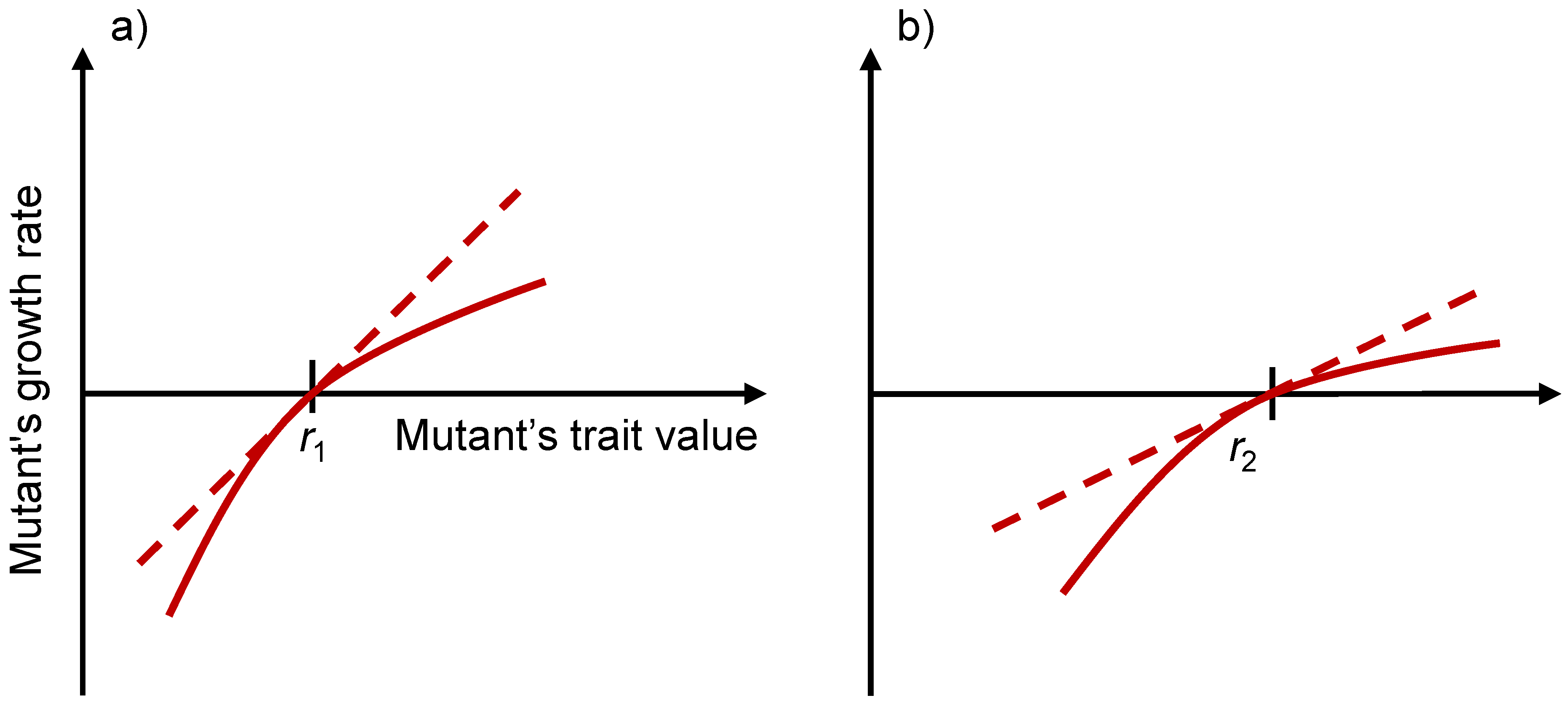
Convergence stable strategySingular strategy that, within a neighborhoods, is approached gradually.
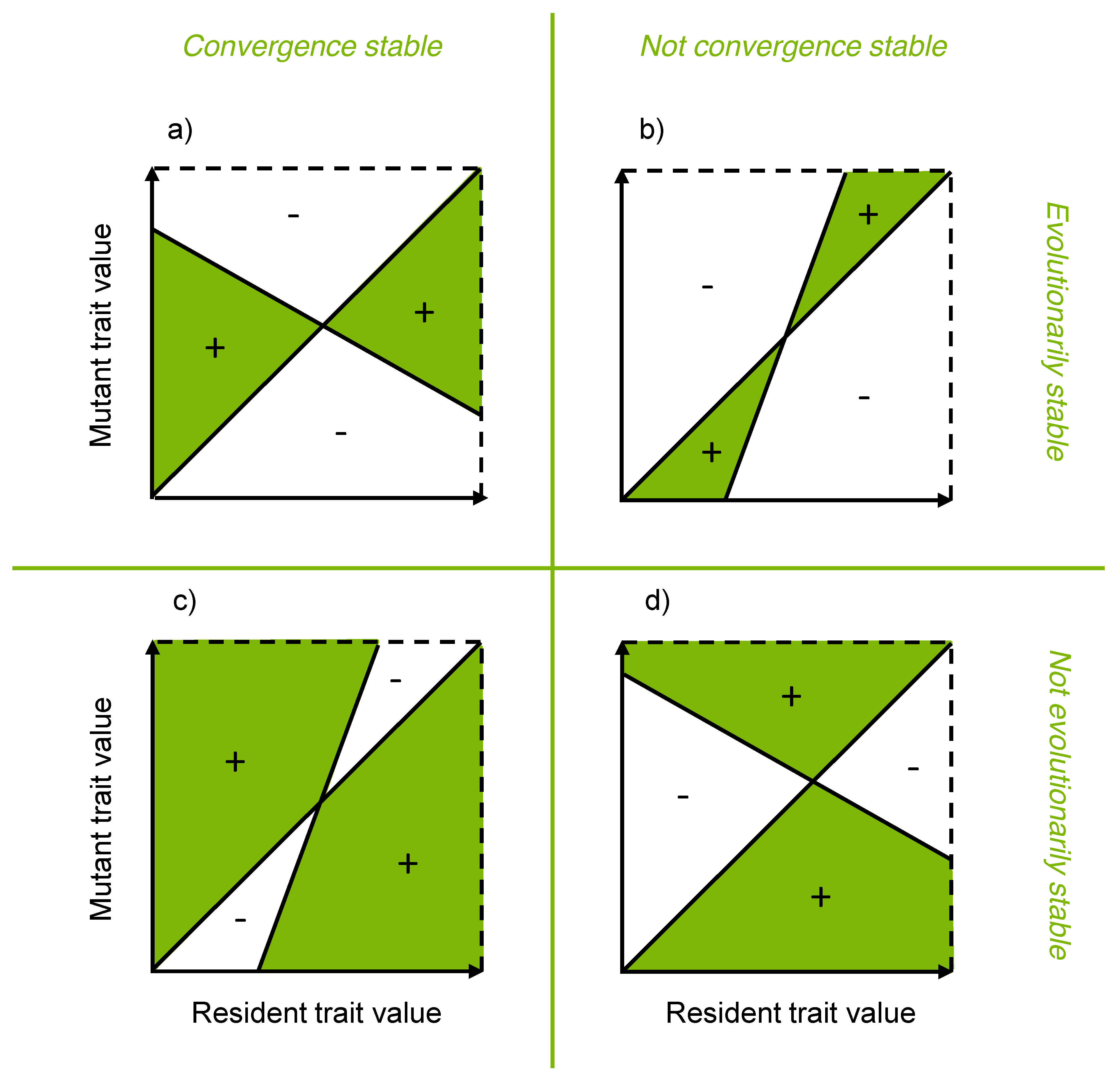
Continuously stable strategy (CSS)Singular strategy that is both convergence stable and evolutionarily stable.
Dimorphic populationPopulation with individuals having either of two distinct trait values.
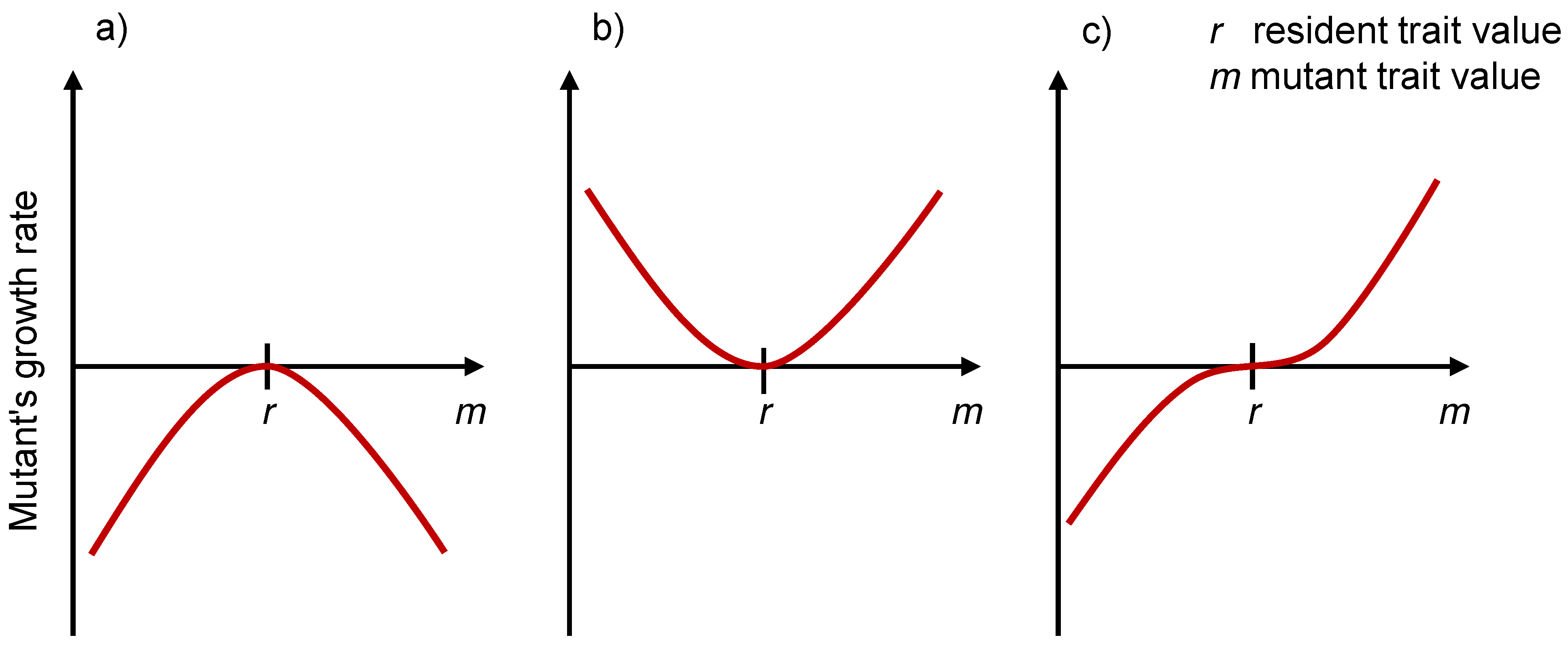
Evolutionarily singular strategyTrait value at which the selection gradient vanishes.
Evolutionarily stable strategy (ESS)Trait value that cannot be invaded by any nearby mutant.
Invasion fitnessThe expected growth rate of a rare mutant.
Monomorphic populationPopulation consisting of individuals with only one distinct trait value.
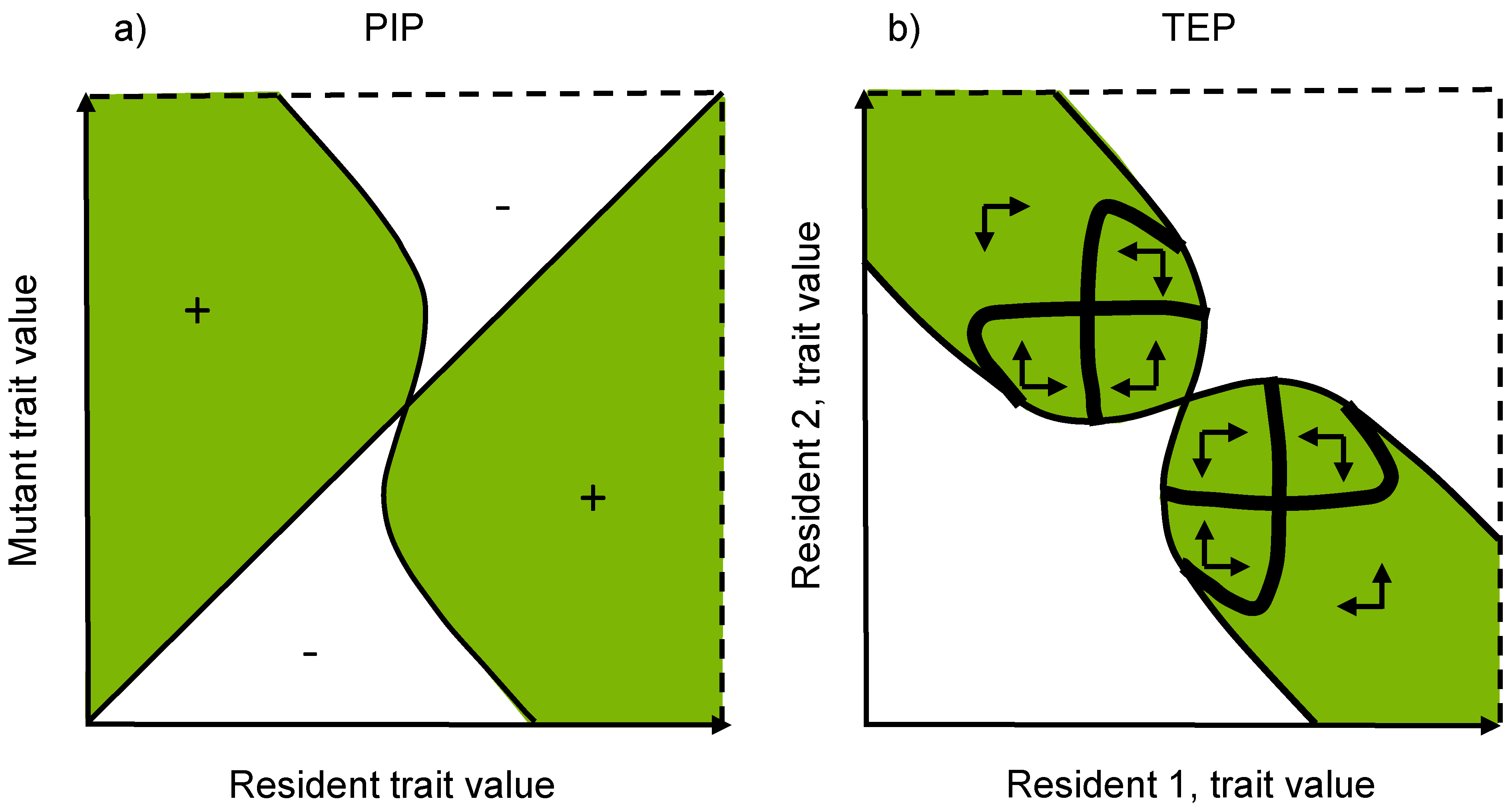
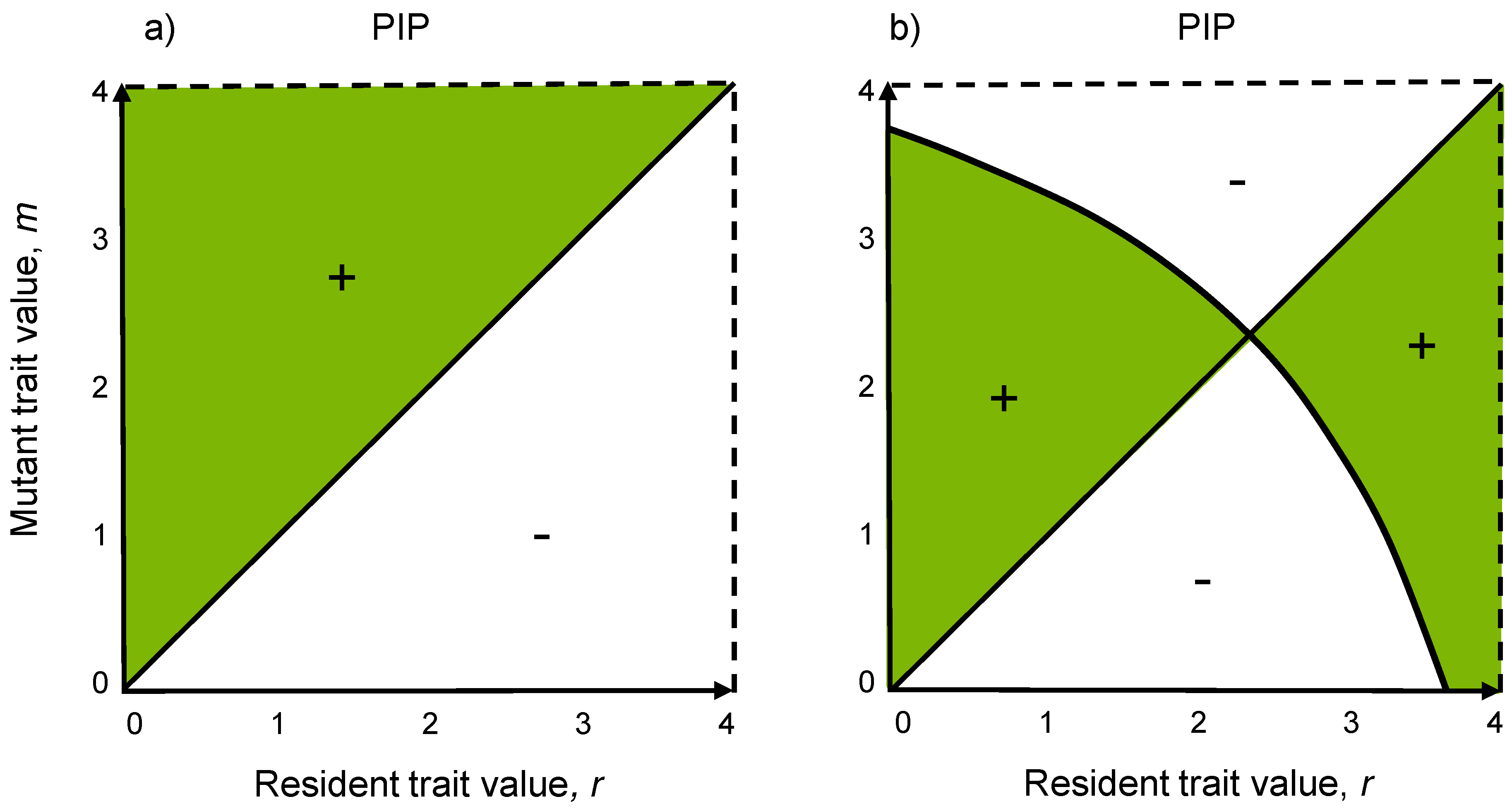
Pairwise invasibility plot (PIP)Graphical illustration of invasion success of potential mutants when the population is monomorphic.
Per capita growth rateThe expected rate at which an individual produces offspring. Can be determined by dividing the population growth rate by the number of individuals.
Polymorphic populationPopulation with individuals having either of several distinct trait values.
Selection gradientSlope of the invasion fitness at the resident trait value. Gives information on the direction and speed of evolutionary change.
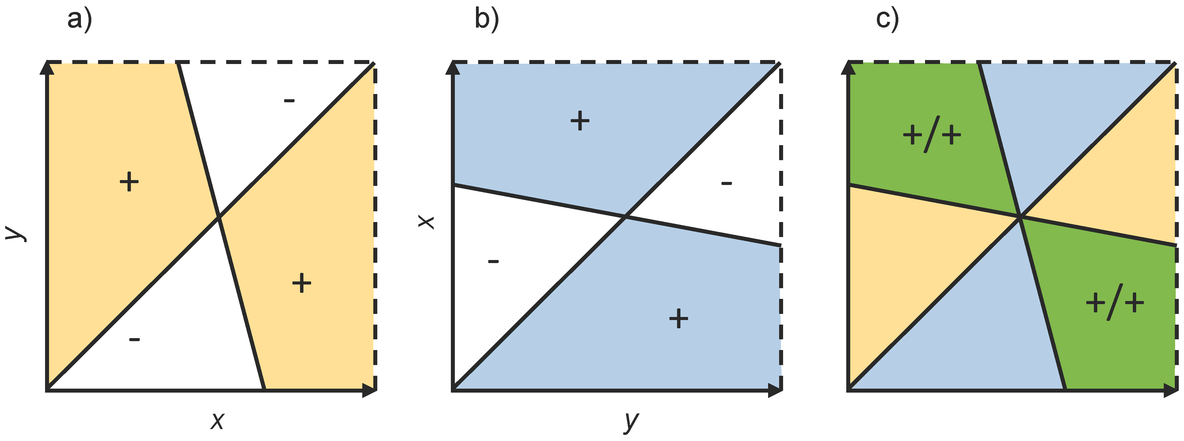
Trait evolution plot (TEP)Graphical illustration of invasion success of potential nearby mutants when the population is dimorphic.

3. Monomorphic Evolution

To see how the fundamental concepts introduced above are used, it makes sense to start with the simplest case of a monomorphic population, i.e., a population that consists of individuals with identical trait values. If not explicitly stated differently, we will assume a single trait value and we write r and m for the trait value of the monomorphic resident population and that of an invading mutant respectively.

3.1. Invasion Fitness and the Selection Gradient

The invasion fitness s r ( m ) is defined as the expected per capita growth rate of an initially rare mutant in the environment set by the resident, which simply means the frequency of each trait value whenever this suffices to infer all other aspects of the equilibrium environment, such as the demographic composition and the availability of resources. For each resident trait value r, the invasion fitness can be thought of as the fitness landscape experienced by initially rare mutants. Importantly, the fitness landscape changes with each successful invasion (see Figure 1), in contrast to the classical view of evolution as an optimization process towards ever higher fitness.
Figure 1. Plot of the invasion fitness s r ( m ) , the expected growth rate of a rare mutant in the environment set by the resident (solid lines), as a function of the mutant trait value m, for two illustrative cases. The dashed lines denote the local tangent of s r ( m ) at m = r where its slope corresponds to the selection gradient s r ( r ) . (a) The population is monomorphic and consists only of individuals with trait value r 1 . Mutants with higher trait values have positive expected growth rate and can hence invade. (b) A mutant with trait value r 2 has invaded and successfully replaced the resident. Since the population now consists of individuals with a new trait value, r 2 , the fitness landscape itself has changed. Note that the invasion fitness vanishes exactly when the mutant trait value equals that of the resident, i.e., m = r 1 and m = r 2 for panel (a) and (b) respectively.
Games 04 00304 g001
We will always assume that the resident is at its demographic attractor, and as a consequence s r ( r ) = 0 for all r as otherwise the population would grow indefinitely.
The selection gradient is defined as the slope of the invasion fitness at m = r , s r ( r ) (see Figure 1). If the sign of the selection gradient is positive (negative), mutants with slightly higher (lower) trait values may successfully invade. This follows from the linear approximation s r ( m ) s r ( r ) ( m r ) , which holds whenever m r . Assuming that mutations are small such that they occur relatively close to the resident trait value, the selection gradient thus determines the direction of evolutionary change.

3.2. Deriving the Invasion Fitness and the Selection Gradient from a Demographic Model

To illustrate the concepts introduced above, consider a population of n individuals that reproduce at a rate b and succumb at the density-dependent rate d n . The number of individuals n ( t ) at time t then grows logistically according to the differential equation n ( t ) = n ( t ) ( b n ( t ) d ) . The equilibrium population density n * is found by solving 0 = n * ( b d n * ) with the non-trivial solution n * = b / d . Though not relevant here, we note that the number of parameters can be reduced to 1 through a change of unit (see e.g., [32,33]).
Next, assume that the birth-rate is subject to evolutionary change without constraints. For this end, we extend the model to include two populations, a resident population n r and a mutant population n m with respective birth rates r and m. Writing n ( t ) = n r ( t ) + n m ( t ) for the total population size we have
n r ( t ) = n r ( t ) r d n t ,
n m ( t ) = n m ( t ) m d n t .
The outcome of competition between the resident and the mutant population can in principle be determined by analyzing the dynamical system above. In this stylized system, that approach actually works. For more complex systems, a rigorous mathematical analysis usually requires a major effort, if it does not fail outright. An adaptive-dynamics analysis sidesteps this difficulty by assuming that the mutant is initially so rare that it has no impact on the per capita growth rates and that the resident is at its demographic equilibrium, i.e., we assume that n ( t ) = n r ( r ) and n r ( t ) = r / d respectively. We now define the invasion fitness s r ( m ) of the mutant as its per capita growth rate n m / n m under these two simplifying assumptions,
s r ( m ) = n m ( t ) n m ( t ) = m d n ( t ) = m r .
At this point, it is useful to verify that s r ( r ) = 0 and that the mutant population size n m ( t ) does not appear in the expression for the invasion fitness. We must have s r ( r ) = 0 since a mutant identical to the resident would on average neither grow nor decline in numbers, and n m ( t ) cannot appear in the invasion fitness since we have assumed the mutant to be so rare that it has no impact on the per-capita growth rates2. We can now find the selection gradient by differentiating with respect to the mutant trait value m and evaluating at the resident trait value m = r . This yields,
s r ( r ) = 1 0 = 1 .
As expected, the birth rate would in this example evolve towards ever higher values. We can change this by introducing a mortality cost c ( r ) of higher birth rates,
n r ( t ) = n r ( t ) r c ( r ) d n t ,
n m ( t ) = n m ( t ) m c ( m ) d n t ,
yielding through the same steps as above the invasion fitness
s r ( m ) = m c ( m ) r + c ( r ) .
Again, we verify that s r ( r ) = 0 . The selection gradient finally becomes:
s r ( r ) = 1 c ( r ) ,
which shows that the selection gradient vanishes (i.e., is equal to 0) when c ( r ) = 1 .

3.3. Evolutionarily Singular Strategies and the Fitness Landscape

What will happen if s r ( r ) vanishes? Seemingly, evolution should come to a halt at such a point. While this is a possible outcome, the general situation is more complex. Traits or strategies r * for which s r * ( r * ) = 0 are known as evolutionarily singular strategies. Near such points the fitness landscape as experienced by a rare mutant is locally “flat”. Figure 2 shows the three qualitatively different ways in which this can occur. Of these, only the two non-degenerate cases corresponding to fitness maxima and fitness minima are of interest here. This is because, in degenerate cases, finite evolutionary steps would lead past the local “flatness”. Figure 2a shows a fitness maximum. This is known as an evolutionarily stable strategy (ESS)3 because, once it is established, it cannot be invaded by nearby mutants. In contrast, Figure 2b shows a fitness minimum at which disruptive selection will occur and the population eventually branches into two morphs and thus becomes dimorphic. This process, known as evolutionary branching, will be further discussed in Section 5.2.
Figure 2. Three qualitatively different singular strategies. (a) A local fitness maximum representing a possible endpoint of evolutionary change. (b) A local fitness minimum at which evolutionary branching can occur. (c) A degenerate case where the criteria from Section 3.5 fail because the second order derivative of s r ( m ) vanishes. These cases are without real-world significance, since finite evolutionary steps will lead evolution past these points.
Games 04 00304 g002

3.4. Pairwise Invasibility Plots

The evolutionary dynamics can be studied graphically. Recall that the invasion fitness represents the fitness landscape as experienced by a rare mutant. In a large (effectively infinite) population, only mutants with trait values m for which s r ( m ) is positive are able to successfully invade. The usual outcome of a successful invasion is that the mutant replaces the resident, and the fitness landscape as experienced by a rare mutant changes. Pairwise invasibility plots (PIPs) are often used to study the consequences of a series of invasions. These plots show, for each resident trait value r, all mutant trait values m for which s r ( m ) is positive. Figure 3 shows PIPs corresponding to the example birth-death model considered in Section 3.2. The green area marked with “+” corresponds to pairs r and m for which a mutant with trait value m can successfully invade a resident population with trait value r, i.e., for which s r ( m ) > 0 . Note that s r ( m ) is zero along the diagonal m = r . In these PIPs, the fitness landscapes as experienced by a rare mutant (see Figure 1) correspond to vertical lines along which the resident trait value r is constant.
Figure 3. Pairwise invasibility plots (PIPs) of the example birth-death model in Section 3.2 with birth rate as the evolving trait value. Green regions represent combinations ( r , m ) for which a mutant with trait value m can invade a resident population consisting of individuals with trait value r, i.e., for which s r ( m ) > 0 . (a) PIP without constraints in birth rate, as given by (1). The birth rate can evolve to ever higher values. (b) PIP with costs of higher birth rate, as given by (2) with c ( r ) = 10 1 exp ( r ) . The singular point is both evolutionarily and convergence stable and is located at r 2 . 3 . Note that diagonal corresponds to s r ( r ) = 0 .
Games 04 00304 g003
Figure 4. Four logical combinations of evolutionary stability and convergence stability for a singular strategy. (a) Evolutionarily stable and convergence stable. A possible endpoint of evolution: the strategy can be attained gradually and then it will resist any invaders successfully. (b) Evolutionarily stable but not convergence stable. Such singular strategies should rarely be realized in nature: although the strategy cannot be invaded once it is realized, evolution starting from any nearby strategy will gradually lead away from the singular strategy. (c) Convergence stable but not evolutionarily stable. A scenario where a population can become dimorphic: the singular strategy can be established gradually, but then it can be invaded by mutants both above and below the resident strategy at the same time. (d) Neither evolutionarily stable nor convergence stable. As in (b), a monomorphic population will evolve away from the singular strategy. It is still possible that a dimorphic population will arise, if coexistence is supported (see Section 5), but it is likely to happen through a large mutational step rather than the gradual process of evolutionary branching.
Games 04 00304 g004
The evolutionarily singular strategies in a PIP are found where the boundary of the region of positive invasion fitness intersects the diagonal. The singular strategy in Figure 4b is a fitness maximum, i.e., an evolutionarily stable strategy, since the invasion fitness is negative both above and below the singular strategy. It is also a convergence stable strategy since nearby monomorphic populations can be invaded by mutants closer to the strategy (i.e., it is an attractor of monomorphic evolutionary dynamics with small mutational steps). Figure 4 shows that all four logical combinations of evolutionary stability and convergence stability can be realized. The singular strategies in the two PIPs in the first row are evolutionarily stable while those in the second column are convergence stable. A singular strategy that is both evolutionarily stable and convergence stable is a possible endpoint of evolutionary change, while a convergence stable strategy that is a fitness minimum is an evolutionary branching point at which the population eventually becomes dimorphic.

3.5. Evolutionary Stability Analysis

Singular strategies can be located and classified once the invasion fitness is known. To locate singular strategies, it is sufficient to find the points for which the selection gradient vanishes, i.e., to find r * such that s r * ( r * ) = 0 . These can be then classified using the second derivative test from basic calculus. If the second derivative of the invasion fitness evaluated at m = r * is negative (positive), the strategy represents a local fitness maximum (minimum). Hence, for an evolutionarily stable strategy r * we have
s r * ( r * ) < 0 .
If this does not hold, the strategy is evolutionarily unstable and, provided that it also convergence stable, evolutionary branching will eventually occur. For a singular strategy r * to be convergence stable, monomorphic populations with slightly lower or slightly higher trait values must be invadable by mutants with trait values closer to r * . For this to happen, the selection gradient s r ( r ) must be positive in a neighborhood of r * for r < r * and negative for r > r * . This means that the slope of the selection gradient s r ( r ) as a function of r at r * is negative, or equivalently that
d d r s r ( r ) | r = r * < 0 .
The criterion for convergence stability given above can also be expressed using second derivatives of the invasion fitness, and the classification can be refined to span more than the simple cases considered here, as discussed in Appendix A (see also Metz et al. [26] and Geritz et al. [27]). However, for practical purposes, the concept of singular strategies as points where the invasion gradient vanishes and the basic criteria given by equations (3) and (4) for evolutionary and convergence stability are often sufficient.

3.6. Modeling Gradual Evolution

The evolutionary process can be envisaged as a sequence of successfully established mutations. This process is strictly directional in large populations as only mutants with positive invasion fitness can invade. The most common way to model directional evolutionary change is a differential equation on the form,
r ( t ) = C s r ( r ) ,
in which the trait value evolves in the direction of positive invasion fitness. The nature of the coefficient C depends on the assumptions that are made about the evolutionary process, but it is always positive and will thus not affect the final evolutionary outcome.
The most common assumption in adaptive dynamics is mutation-limited evolution with small mutational steps. Under these assumptions, Dieckmann and Law [25] (see also Champagnat et al. [35]) have shown that the coefficient C equals the product of the mutation rate, mutation variance, population size, and a factor 1/2 (as, on average, only half of all mutations that arise have positive invasion fitness and thus a chance of being established). The dynamical system with this coefficient is known as the canonical equation of adaptive dynamics. A structurally similar equation applicable to sexually reproducing populations have been introduced in the context of quantitative genetics by Lande [2] and later extended to frequency-dependent selection by Iwasa et al. [36].
While the canonical equation is often used to study evolutionary change, this is by no means necessary. In many cases, the eventual evolutionary outcome is independent of mutational step size and can for monomorphic evolutionary dynamics be determined directly from the pairwise invasibility plot. For polymorphic populations, Ito and Dieckmann [37] have developed an oligomorphic stochastic model for the evolutionary dynamics (see also Dieckmann et al. [38]). An efficient implementation of this method for small mutational steps, which make use of a second-order approximation of the invasion fitness landscape, is given by Brännström et al. [9]. Recently, Sasaki and Dieckmann [39] have developed a framework termed oligomorphic dynamics that brings adaptive dynamics closer to quantitative genetics.

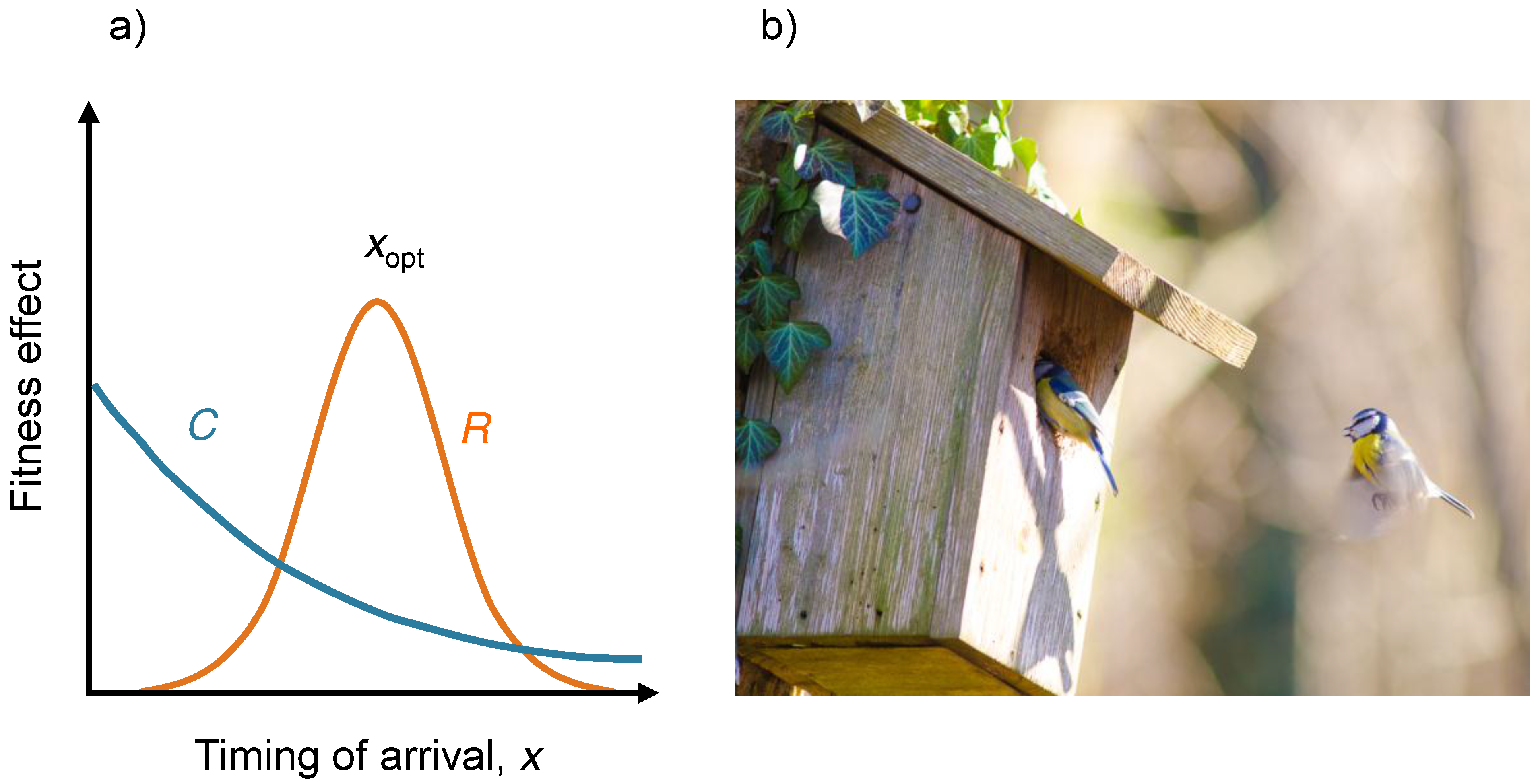
4. Example: Evolution of Arrival Time of Migratory Birds

To illustrate how the introduced techniques for analyzing evolutionary change can be used in practice, we here analyze a simplified variant of a model from Johansson and Jonzén [40]. This example also illustrates how to work with models in discrete time. The model describes the evolution of arrival times of migratory birds at their breeding grounds. Early arrival compromises reproductive success by subjecting adults to harsh winter-like conditions. By arriving late, on the other hand, birds may miss the peak abundance of easily accessible insect larvae to feed their young. One might think that evolution should cause birds to arrive at the time that is optimal for the population, but as we will see, competition between individuals for nesting sites causes birds to arrive earlier while conditions are still harsh.
We write x for the arrival time of a resident population of migratory birds and assume that the birds compete among each other for a total of K available territories. Missing out on a territory means foregoing reproduction that year, so competition for territories is expected to be intense. We assume that the probability of securing a territory is proportional to a birds competitive ability C ( x ) and that a bird with a territory gives rise to an average of R ( x ) offspring. A life-history trade-off now arises if we assume that C ( x ) decreases with the arrival time x, giving a competitive advantage to early-arriving birds, while R ( x ) has a maximum at an optimal arrival time x opt . At what time should a bird arrive to maximize its expected reproductive success?
To answer this question, we first assume that there are more individuals than available territories and that individuals survive from one year to the next with probability p. The demographic dynamics of the resident is then simply
n t + 1 = K R ( x ) + p n t .
We find the fixed point by substituting n t + 1 = n t = n * , which gives n * = K R ( x ) / ( 1 p ) . It is easy to verify that the fixed point is stable4. Note that the arrival time that maximizes the population size is x opt .
We now consider an invasion by a mutant bird with population size n t and arrival time x , giving the joint demographic dynamics
n t + 1 = K n t C ( x ) n t C ( x ) + n t C ( x ) R ( x ) + p n t , n t + 1 = K n t C ( x ) n t C ( x ) + n t C ( x ) R ( x ) + p n t .
As the dynamical system is in discrete time, we define the invasion fitness w x ( x ) as the yearly growth rate (geometric growth rate) of an initially rare mutant. It should be noted that the discrete-time invasion fitness w is dimensionless, unlike the continuous-time counterpart s, which has unit 1 / time . The two are related as s = ( log w ) / Δ t , where Δ t is the time interval on which the discrete-time invasion fitness is based,
Assuming that the resident is at its demographic attractor and that the mutant is so rare that it has a negligible influence on per capita growth rates, we have
w x ( x ) = n t + 1 n t = K C ( x ) n * C ( x ) R ( x ) + p = ( 1 p ) C ( x ) R ( x ) C ( x ) R ( x ) + p .
Since we are basing the invasion fitness on the yearly geometric growth rate, the condition that corresponds to the assumption that the resident is at its demographic equilibrium is w x ( x ) = 1 . It is easily verified that this is the case, so we can feel more confident in the correctness of our derivation.
Next, we determine the selection gradient. Differentiating the invasion fitness with respect to the mutant trait value x and evaluating at x = x , we get
w x ( x ) = ( 1 p ) C ( x ) C ( x ) + R ( x ) R ( x ) .
A later arrival time is favored whenever the relative decrease in competitive ability, C ( x ) / C ( x ) , is smaller than the relative increase in reproductive success, R ( x ) / R ( x ) . We can thus see selection is a tug of war between the need to secure a territory and the desire to maximize the number of offspring from the breeding site.
To move further, we make the specific assumption that the competitive ability decreases exponentially with arrival time and that the reproductive success of territory owners is given by a Gaussian function (see Figure 5),
C ( x ) = exp ( a x ) and R ( x ) = R 0 exp x x opt 2 2 σ 2 ,
where R 0 is the maximal reproductive output, x opt is the optimal arrival time for reproduction, and σ corresponds to the length of the benign summer-like season. Using that C ( x ) = a C ( x ) and R ( x ) = ( x x opt ) R ( x ) / σ 2 , we get
D ( x ) = w x ( x ) = ( 1 p ) a + x x opt σ 2 .
The selection gradient is linear and decreasing so there is exactly one evolutionarily singular strategy, which must be convergence stable. Solving D ( x * ) = 0 for this singular strategy gives x * = x opt a σ 2 . A direct calculation now shows that w x * ( x * ) < 0 so x * is an evolutionarily stable strategy, in fact a continuously stable strategy.
Figure 5. In many territorial animals, there is a prior residence effect by which the first individual to occupy a territory often gets the upper hand in the competition. (a) In the model in Section 4, it is assumed that reproductive output E (orange line) is maximized for arrival at day x opt . Early-arriving individuals have a higher competitive ability C (blue line), which makes them more able to obtain territories. (b) Two individuals of blue tit (Cyanistes caeruleus), a partial migratory bird, competing over a nest box in the beginning of the breeding season (photo: Niclas Jonzén).
Games 04 00304 g005
We conclude that, due to the individual advantage of arriving earlier relative to the rest of the population, the evolutionarily stable strategy occurs some time before the arrival date x opt that maximizes the population size. This is an example of the tragedy of the commons in evolution (cf. [41]).

5. Polymorphic Evolution

The normal outcome of a successful invasion is that the mutant replaces the resident. However, other outcomes are also possible ([42]), in particular both the resident and the mutant may persist and the population then becomes dimorphic. Assuming that a trait persists in the population if and only if its expected growth-rate when rare is positive, the condition for coexistence among two traits r 1 and r 2 is
s r 1 ( r 2 ) > 0 and s r 2 ( r 1 ) > 0 ,
where r 1 and r 2 are often referred to as morphs. Such a pair is a protected dimorphism. The set of all protected dimorphism is known as the region of coexistence. Graphically, the region of coexistence consists of the overlapping parts when a pairwise invasibility plot is mirrored over the diagonal (see Figure 6).
Figure 6. Illustration of the graphical method for obtaining the region of coexistence. (a) A pairwise invasibility plot from the Snowdrift game [10]. (b) The same pairwise invasibility plot mirrored over the main diagonal. (c) The first two panels overlaid in which the region of coexistence is visible as the green (dark gray) area. Note that protected dimorphisms are possible even though the singular strategy is evolutionarily stable and selection thus stabilizing.
Games 04 00304 g006

5.1. Invasion Fitness and Selection Gradients in Polymorphic Populations

The invasion fitness is generalized to dimorphic populations in a straightforward manner, as the expected growth rate s r 1 , r 2 ( m ) of a rare mutant in the environment set by the two morphs r 1 and r 2 . The slope of the local fitness landscape for a mutant close to r 1 or r 2 is now given by the selection gradients
s r 1 , r 2 ( r 1 ) and s r 1 , r 2 ( r 2 ) .
In practice, it is often difficult to determine the invasion fitness analytically, and one often has to resort to numerical analysis.

5.2. Evolutionary Branching

The emergence of protected dimorphism near singular strategies during the course of evolution is not unusual, but its significance depends on whether selection is stabilizing (invasion-fitness maximum) or disruptive (invasion-fitness minimum). In the latter case, the traits of the two morphs will diverge in a process often referred to as evolutionary branching. Metz et al. [26] and Geritz et al. [27] present a compelling argument that disruptive selection only occurs near fitness minima. To understand this heuristically, consider a dimorphic population r 1 and r 2 near a singular strategy which is a fitness maximum. By continuity s r ( m ) s r 1 , r 2 ( m ) and, since s r 1 , r 2 ( r 1 ) = s r 1 , r 2 ( r 2 ) = 0 , the fitness landscape for the dimorphic population must be a perturbation of that shown in Figure 2a with the region of positive invasion fitness between r 1 and r 2 . Selection is thus stabilizing.

5.3. Trait Evolution Plots

Evolution after evolutionary branching is illustrated using trait evolution plots. These show the region of coexistence, the direction of evolutionary change, and whether strategies at which the selection gradient vanishes are fitness maxima or minima. Evolution may well drive the dimorphic population outside the region of coexistence, in which case one morph goes extinct and the population once again becomes monomorphic.
Figure 7. Levene’s soft selection model studied by Geritz et al. [27]. (a) Pairwise invasibility plot showing the evolutionary dynamics for a monomorphic population. Since selection at the convergence stable singular strategy is disruptive, the population eventually becomes dimorphic with evolutionary dynamics given by the trait evolution plot. (b) Trait evolution plot showing the direction of evolutionary change. Thick lines are evolutionarily stable isoclines, where directional selection in one of the two morphs ceases. In this case, the trait evolution plot shows the final evolutionary outcome to be a stable protected dimorphism located at the intersection of the two isoclines. The green area is the region of coexistence, as described in Figure 6.
Games 04 00304 g007
Figure 7 shows an example of a trait evolution plot. The lines are evolutionary isoclines where one of the two selection gradients vanishes. These are found by solving
s r 1 , r 2 ( r 1 ) = 0 or s r 1 , r 2 ( r 2 ) = 0 .
An isocline can be either a fitness maximum or fitness minima for mutants close to the morph (in fact the situation is exactly identical to the monomorphic case if we consider the other morph as being a constant part of the environment). We recommend using the same conventions as Geritz et al. [27], that is, using thin lines to denote fitness minima, and thick lines for fitness maxima.

5.4. Evolutionarily Singular Coalitions

An intersections of two isoclines is known as a singular coalition ([26,27]). If the strategies r 1 and r 2 at the intersection are evolutionarily stable strategies when considered separately with the other trait value fixed, the coalition is not invadable and represent a possible endpoint where evolutionary change ceases. To test for stability, the analytical condition for evolutionary stability can be applied to each morph, however there is no single natural generalization of a convergence stable strategy ([26,27]) and convergence stability is in practice often most easily inferred directly from the trait evolution plot. See Leimar [43] for a detailed discussion of convergence stability in multidimensional trait spaces.

5.5. Connection of the Isoclines to the Boundary

The boundaries of the region of coexistence are extinction threshold for morphs, and hence for a dimorphic population r 1 and r 2 the boundary where r 2 becomes extinct is given implicitly by s r 1 ( r 2 ) = 1 and for points in the region of coexistence close to this boundary the approximate relationship s r 1 , r 2 ( m ) s r 1 ( m ) holds. This simple observation has implications for the connection of the isoclines to the boundary. If s r 1 , r 2 ( r 1 ) = 0 on the boundary we also have s r 1 ( r 1 ) = 0 , so r 1 must be a singular strategy of a monomorphic population.
The isoclines defined by s r 1 , r 2 ( r 2 ) = 0 connects to the boundary where it has a vertical tangent. The reason is that at every other point on the boundary, the selection gradient for r 2 points towards the interior of the region of coexistence (either up or down). If the isocline would connect to such a point, it would divide the region into two areas where the selection gradient for r 2 points in opposing directions, and one of these would not be towards the interior, which is a contradiction. By symmetry we get corresponding results for the other isoclines. For a more detailed discussion see Geritz et al. [27].

5.6. Further Evolutionary Branching

Evolutionary branching in a morph r 1 under small but fixed mutational steps may occur whenever the fitness landscape as given by the function s r 1 , r 2 ( m ) has a local minimum at r 1 . The most likely evolutionary branching point is an invadable singular coalition, but evolutionary branching could also happen along an isocline if the community stays close enough for a sufficiently long time, as might be the case when the isocline is nearly vertical or horizontal. In other cases, directional selection is likely to move the community away from the isocline before the process of evolutionary branching can unfold.

6. Discussion

It is late afternoon and only hours remain until we have to cease writing and submit this manuscript for publication. Thankfully, most of what we have wanted to say has already been presented in the previous sections and all that remains is now to give our personal views on two selected topics and to offer recommendations for further reading on the rapidly developing field of adaptive dynamics.

6.1. Relation to Evolutionary Game Theory

The archetypal situation in evolutionary game theory is a population of individuals choosing between two or more pure strategies. The classical hawk-dove game, introduced by Maynard Smith and Price [44], assumes pairwise encounters between individuals. In each such encounter, an individual acts aggressively (hawk) with probability r and timidly (dove) with probability 1 r . The frequencies of the strategies conventionally change according to the replicator equations. Although these equations do not consider the density of individuals, it is possible to derive an invasion fitness using adaptive dynamics techniques (see Appendix B of Brännström et al. [13] for an example of how the replicator equations can be derived from an underlying demographic model). This invasion fitness then has the following form,
s r ( m ) = m P H ( r ) + ( 1 m ) P D ( r ) ,
in which P H ( r ) and P D ( r ) are the frequency-dependent payoffs corresponding to the pure hawk and pure dove strategy respectively. The key aspect to note is that the invasion fitness is linear in the mutant trait value. As a direct consequence, it vanishes entirely at evolutionarily singular strategies. It is no longer possible to talk about fitness minima or maxima and subtle second-order techniques that consider a finite but small number of mutant individuals are needed to assess whether the singular strategy is evolutionarily stable. In evolutionary game theory, the vanishing fitness landscape is enshrined in the Bishop–Cannings theorem ([45]). In the unifying framework of adaptive dynamics, it is but a degeneracy that arises because the invasion fitness is linear in the mutant trait value. For further reading on the relation between adaptive dynamics and evolutionary game theory, we recommend Meszéna et al. [46] and Dieckmann and Metz [47].

6.2. Role in Speciation Research

One of the most exciting findings of adaptive dynamics is evolutionary branching, the process by which an initially monomorphic population can become dimorphic through small mutational steps (see Section 5.2). If individuals in a sexually reproducing population are sufficiently picky in their choice of mates, a similar scenario unfolds as demonstrated by Dieckmann and Doebeli [6]. That being said, the likelihood that this process would unfold in nature remains vigorously debated. One of the most important contested points concerns whether the required degree and cost of assortative mating can realistically be expected in natural populations (see, e.g., Gavrilets [48]).
We do not wish to place ourselves in the line of fire. Rather, we want to highlight the usefulness of adaptive dynamics in elucidating the ecological conditions that support species coexistence over evolutionary timescales. In the classical picture of speciation, an ancestral population becomes spatially separated. The two populations evolve in different directions and, over time, they might accumulate Dobzhansky–Muller incompatibilities. If, at some later time, these populations come into secondary contact, the potentially accumulated incompatibilities would severely reduce the fitness of any hybrid offspring, so-called post-zygotic isolation. Selection might then promote mechanisms that prevent the formation of hybrid offspring, so-called pre-zygotic isolation. In this scenario, two new species have emerged from one.
The above process, known as allopatric speciation, could conceivably work if the population becomes spatially segregated and the environments that the two subpopulations encounter are sufficiently different, for example if they contain different resources, henceforth apples and pears. Should the two environments contain both apples and pears, which we find more likely, the story would be more complicated. It would take a stroke of luck to ensure that one subpopulation specializes on apples with the other specializing on pears. An outcome that we find more plausible is that two subpopulations remain generalists, consuming both apples and pears. They might still acquire Dobzhansky–Muller incompatibilities and pre-zygotic isolation could potentially evolve upon secondary contact. What comes next, however, depends on the ecology. Under disruptive selection, we might see the emergence of two ecologically differentiated species. The period in allopatry has then become the tool that facilitates evolutionary branching, but the ecological side of the story remains unchanged.
Complete spatial segregation is probably unlikely and several mechanisms exist that can enable speciation in the presence of some degree of gene flow ([49]). This includes divergence hitchhiking and genomic hitchhiking that suppresses the effective migration rates for genes in part or in all of the genome ([50]), and genomic conflict that might facilitate reproductive isolation ([51]). In all of these cases, adaptive dynamics is useful for understanding when the ecology would facilitate divergence and the eventual coexistence of species over evolutionary time scales. A concerted use of adaptive dynamics and quantitative genetics would furthermore enable different scenarios of speciation to be tested and critically compared. In this sense, adaptive dynamics should have an important role to play in modern speciation research.

6.3. Recommendations for Further Reading

A good introductory text to adaptive dynamics is Diekmann [52], which presents the basics of monomorphic evolution using many instructive examples. The next natural step is Metz et al. [26] and Geritz et al. [27], which describe the theory in depth. To better understand how the techniques can be used in studying more complex models, a manuscript studying a sample model such as Geritz et al. [53] or Brännström and Dieckmann [11] may prove helpful. The latter work builds on techniques presented in Brännström and Sumpter [54] and the results have been generalized in Brännström et al. [9]).
The canonical equation is introduced by Dieckmann and Law [25], studied in more detail by Champagnat et al. [35] and extended to physiologically structured populations by Durinx and Metz [55] and Durinx et al. [56]. Champagnat et al. [57] puts this into context by comprehensively considering different ways in which microscopic stochastic processes can be studied on a macroscopic scale.
Several extensions of adaptive dynamics have been considered over the last two decades. Table 2 gives a selected overview of some of the more prominent developments. A list of articles related to adaptive dynamics is also maintained by Eva Kisdi at mathstat.helsinki.fi/~kisdi/addyn.htm. Adaptive dynamics is an active area of research, so be sure to check the forward citations for the latest developments.
Table 2. Salient extensions of adaptive dynamics theory ordered according to topic.
Type of generalizationReferences
Explicit genetics and standing genetic variation[39,58,59,60,61]
Mathematical underpinnings[42,62,63,64,65]
Multiple species[9,66,67,68]
Multiple traits and function-valued traits[43,69,70,71]
Physiologically structured populations[55,56]
Sexually-reproducing populations[72]
Spatially-structured populations[73,74,75]
Stochastic environments[76,77,78]
Trade-off analysis[79,80,81,82,83]

Acknowledgments

Acknowledgments We thank Bernd Blasius and Thilo Gross for inviting us to the Stanislaw Lem workshop on evolution at Lviv, Ukraine in 2005. Following this workshop, we started writing the Hitchhiker’s Guide to Adaptive Dynamics. At this time, Å.B. was a postdoctoral fellow in Nara, Japan, supported by a generous grant from the Japan Society for the Promotion of Science. This support is gratefully acknowledged. We also want to thank Ulf Dieckmann, Hans Metz, Karl Sigmund, and Fugo Takasu for countless discussions about adaptive dynamics and its applications, as well as Niclas Jonzén for kindly allowing us to reproduce his photo of two blue tits competing for a nest box. Finally, we very much appreciate the kind and supportive statements we have received from readers of early versions of this manuscript.

A. Appendix: Local Classification of Singular Strategies

We here give a brief mathematical derivation of criteria that can be used to check whether a singular strategy is evolutionarily stable, convergence stable, and whether protected dimorphisms (two coexisting populations with different trait values) are possibility near the singular strategy. The arguments build on Metz et al. [26] and Geritz et al. [27] and we refer to these papers for further details.
As stated in Section 3.3, a singular strategy r * is evolutionarily stable (an ESS) provided that it is a local maximum of s r * ( m ) . Readers who have taken an introductory course in calculus might recognize that r * is a critical point of s r * ( m ) . The evolutionarily stability can thus be assessed using the second derivative test from calculus. Writing the invasion fitness s r ( m ) as a function of two variables, s r ( m ) s ( r , m ) , we can thus express the ESS criterion as the requirement that the second derivative in the mutant direction evaluated at the singular strategy is positive:
2 s m 2 | r = m = r * < 0 ( ESS criterion ) .
For a singular strategy to be convergence stable, the selection gradient needs to point towards the singular strategy, i.e., its sign must change from positive to negative when going through r * . Hence, the selection gradient s r ( r ) must be a decreasing function near the singular strategy,
d d r s r ( r ) = 2 s r 2 | r = m = r * + 2 s m r | r = m = r * < 0 .
Since s r ( r ) = 0 we have
0 = d d r 2 s r ( r ) = 2 s r 2 | m = r + 2 2 s m r | m = r + 2 s m 2 | m = r
and thus (6) can be rewritten as
2 s r 2 | r = m = r * > 2 s 2 m | r = m = r * ( convergence stability ) .
If a singular strategy is convergence stable but not evolutionarily stable, selection is disruptive near the singular strategy and evolutionary branching will eventually occur. However, even with stabilizing selection, protected dimorphism may occur near a singular strategy provided there are points near the singular strategy where both s ( r , m ) and s ( m , r ) are positive. This means that the line m r * = ( r r * ) passing through the singular strategy at an angle of −45 degrees must locally be in a region where s is positive. Thus, s ( r , 2 r * r ) must have a minimum at r * , meaning that at this point its second derivative is positive. Hence,
2 s m 2 | r = m = r * 2 2 s r m | r = m = r * + 2 s r 2 | r = m = r * > 0 .
which using again (7) gives the criterion
2 s m 2 | r = m = r * > 2 s r 2 | r = m = r * ( dimorphism criterion )
for protected dimorphisms to exist near the singular strategy.

References

  1. Crow, J.F.; Kimura, M. An Introduction to Population Genetics Theory; Harper & Row: New York, NY, USA, 1970. [Google Scholar]
  2. Lande, R. Natural selection and random genetic drift in phenotypic evolution. Evolution 1976, 314–334. [Google Scholar] [CrossRef]
  3. Falconer, D.S.; Mackay, T.F.C. Introduction to Quantitative Genetics, 4th ed.; Prentice Hall: Harlow, UK, 1996. [Google Scholar]
  4. Maynard Smith, J. Evolution and the Theory of Games; Cambridge University Press: Cambridge, UK, 1986. [Google Scholar]
  5. Hofbauer, J.; Sigmund, K. Evolutionary Games and Population Dynamics; Cambridge University Press: Cambridge, UK, 1998. [Google Scholar]
  6. Dieckmann, U.; Doebeli, M. On the origin of species by sympatric speciation. Nature 1999, 400, 354–357. [Google Scholar] [CrossRef] [PubMed]
  7. Doebeli, M.; Dieckmann, U. Speciation along environmental gradients. Nature 2003, 421, 259–264. [Google Scholar] [CrossRef] [PubMed]
  8. Dieckmann, U.; Ferrière, R. Adaptive dynamics and evolving biodiversity. In Evolutionary Conservation Biology; Ferrière, R., Dieckmann, U., Couvet, D., Eds.; Cambridge University Press: Cambridge, UK, 2004; pp. 188–224. [Google Scholar]
  9. Brännström, Å.; Loeuille, N.; Loreau, M.; Dieckmann, U. Emergence and maintenance of biodiversity in an evolutionary food-web model. Theor. Ecol. 2011, 4, 467–478. [Google Scholar]
  10. Doebeli, M.; Hauert, C.; Killingback, T. The evolutionary origin of cooperators and defectors. Science 2004, 306, 859–862. [Google Scholar] [CrossRef] [PubMed]
  11. Brännström, Å.; Dieckmann, U. Evolutionary dynamics of altruism and cheating among social amoebas. Proc. R. Soc. Lond., B, Biol. Sci. 2005, 272, 1609–1616. [Google Scholar]
  12. Sumpter, D.J.T.; Brännström, Å. Synergy in social communication. In Sociobiology of Communication: An Interdisciplinary Perspective; Oxford University Press: Oxford, UK, 2008; pp. 191–208. [Google Scholar]
  13. Brännström, Å.; Gross, T.; Blasius, B.; Dieckmann, U. Consequences of fluctuating group size for the evolution of cooperation. J. Math. Biol. 2011, 63, 263–281. [Google Scholar]
  14. Cornforth, D.M.; Sumpter, D.J.T; Brown, S.P.; Brännström, Å. Synergy and group size in microbial cooperation. Am. Nat. 2012, 180, 296–305. [Google Scholar] [CrossRef] [PubMed]
  15. Dieckmann, U.; Metz, J.A.; Sabelis, M.W.; Sigmund, K. Adaptive Dynamics of Infectious Diseases: In Pursuit of Virulence Management; Cambridge University Press: Cambridge, UK, 2005. [Google Scholar]
  16. Boldin, B.; Diekmann, O. Superinfections can induce evolutionarily stable coexistence of pathogens. J. Math. Biol. 2008, 56, 635–672. [Google Scholar] [CrossRef] [PubMed]
  17. Best, A.; White, A.; Boots, M. The implications of coevolutionary dynamics to host-parasite interactions. Am. Nat. 2009, 173, 779–791. [Google Scholar] [CrossRef] [PubMed]
  18. Svennungsen, T.O.; Kisdi, É. Evolutionary branching of virulence in a single-infection model. J. Theor. Biol. 2009, 257, 408–418. [Google Scholar] [CrossRef] [PubMed]
  19. Parvinen, K. Evolutionary suicide. Acta Biotheoretica 2005, 53, 241–264. [Google Scholar] [CrossRef] [PubMed]
  20. Nonaka, E.; Parvinen, K.; Brännström, Å. Evolutionary suicide as a consequence of runaway selection for greater aggregation tendency. J. Theor. Biol. 2012. [Google Scholar]
  21. Marrow, P.; Dieckmann, U.; Law, R. Evolutionary dynamics of predator-prey systems: An ecological perspective. J. Math. Biol. 1996, 34, 556–578. [Google Scholar] [CrossRef] [PubMed]
  22. Kisdi, É.; Jacobs, F.; Geritz, S. Red Queen evolution by cycles of evolutionary branching and extinction. Selection 2002, 2, 161–176. [Google Scholar]
  23. Dercole, F.; Ferriere, R.; Gragnani, A.; Rinaldi, S. Coevolution of slow–fast populations: Evolutionary sliding, evolutionary pseudo-equilibria and complex Red Queen dynamics. Proc. R. Soc. Lond., B, Biol. Sci. 2006, 273, 983–990. [Google Scholar] [CrossRef] [Green Version]
  24. Metz, J.A.J.; Nisbet, R.; Geritz, S. How should we define “fitness” for general ecological scenarios? Trends Ecol. Evol. 1992, 7, 198–202. [Google Scholar] [CrossRef]
  25. Dieckmann, U.; Law, R. The dynamical theory of coevolution: A derivation from stochastic ecological processes. J. Math. Biol. 1996, 34, 579–612. [Google Scholar] [CrossRef] [PubMed]
  26. Metz, J.A.J.; Geritz, S.A.; Meszéna, G.; Jacobs, F.J.; Van Heerwaarden, J. Adaptive dynamics, a geometrical study of the consequences of nearly faithful reproduction. In Stochastic and Spatial Structures of Dynamical Systems; van Strien, S.J., Verduyn Lunel, S.M., Eds.; North-Holland Publishing Co: Amsterdam, The Netherlands, 1996; pp. 183–231. [Google Scholar]
  27. Geritz, S.A.; Kisdi, E.; Mesze, G.; Metz, J. Evolutionarily singular strategies and the adaptive growth and branching of the evolutionary tree. Evol. Ecol. 1997, 12, 35–57. [Google Scholar] [CrossRef]
  28. McGill, B.J.; Brown, J.S. Evolutionary game theory and adaptive dynamics of continuous traits. Annu. Rev. Ecol. Evol. Syst. 2007, 38, 403–435. [Google Scholar] [CrossRef]
  29. Waxman, D.; Gavrilets, S. 20 questions on adaptive dynamics. J. Evol. Biol. 2005, 18, 1139–1154. [Google Scholar] [CrossRef] [PubMed]
  30. Metz, J.A.J. Adaptive dynamics. In Encyclopedia of Theoretical Ecology; Hastings, A., Gross, L.J., Eds.; University of California Press: Berkeley, US, 2012; Vol. 4, pp. 7–17. [Google Scholar]
  31. Rueffler, C.; Egas, M.; Metz, J.A.J. Evolutionary predictions should be based on individual-level traits. Am. Nat. 2006, 168, 147–162. [Google Scholar] [CrossRef] [PubMed]
  32. Edelstein-Keshet, L. Mathematical Models in Biology; McGraw-Hill Companies: New York, NY, USA, 1988. [Google Scholar]
  33. Bernstein, M.A.; Friedman, W.A. Thinking About Equations; Wiley: New York, NY, USA, 2009. [Google Scholar]
  34. Metz, J.A.J. Thoughts on the geometry of Meso-evolution: Collecting mathematical elements for a postmodern synthesis. In The Mathematics of Darwin’s Legacy; Chalub, F.A., Rodrigues, J.F., Eds.; Birkhäuser: Basel, Germany, 2011; pp. 193–232. [Google Scholar]
  35. Champagnat, N.; Ferrière, R.; Arous, G.B. The canonical equation of adaptive dynamics: A mathematical view. Selection 2001, 2, 73–83. [Google Scholar] [CrossRef]
  36. Iwasa, Y.; Pomiankowski, A.; Nee, S. The evolution of costly mate preferences II. The “handicap” principle. Evolution 1991, 45, 1431–1442. [Google Scholar] [CrossRef]
  37. Ito, H.C.; Dieckmann, U. A new mechanism for recurrent adaptive radiations. Am. Nat. 2007, 170, E96–E111. [Google Scholar] [CrossRef] [PubMed]
  38. Dieckmann, U.; Brännström, Å.; HilleRisLambers, R.; Ito, H.C. The adaptive dynamics of community structure. In Mathematics for Ecology and Environmental Sciences; Springer: Berlin, Germany, 2007; pp. 145–177. [Google Scholar]
  39. Sasaki, A.; Dieckmann, U. Oligomorphic dynamics for analyzing the quantitative genetics of adaptive speciation. J. Math. Biol. 2011, 63, 601–635. [Google Scholar] [CrossRef] [PubMed]
  40. Johansson, J.; Jonzén, N. Game theory sheds new light on ecological responses to current climate change when phenology is historically mismatched. Ecol. Lett. 2012, 15, 881–888. [Google Scholar] [CrossRef] [PubMed]
  41. Rankin, D.J.; Bargum, K.; Kokko, H. The tragedy of the commons in evolutionary biology. Trends Ecol. Evol. 2007, 22, 643–651. [Google Scholar] [CrossRef] [PubMed]
  42. Geritz, S.A.H.; Gyllenberg, M.; Jacobs, F.J.A.; Parvinen, K. Invasion dynamics and attractor inheritance. J. Math. Biol. 2002, 44, 548–560. [Google Scholar] [CrossRef] [PubMed]
  43. Leimar, O. Multidimensional convergence stability. Evol. Ecol. Res. 2009, 11, 191–208. [Google Scholar]
  44. Maynard Smith, J.; Price, G. The logic of animal conflict. Nature 1973, 246, 15. [Google Scholar] [CrossRef]
  45. Bishop, D.; Cannings, C. A generalized war of attrition. J. Theor. Biol. 1978, 70, 85–124. [Google Scholar] [CrossRef]
  46. Meszéna, G.; Kisdi, É.; Dieckmann, U.; Geritz, S.A.; Metz, J.A.J. Evolutionary optimisation models and matrix games in the unified perspective of adaptive dynamics. Selection 2002, 2, 193–220. [Google Scholar] [CrossRef]
  47. Dieckmann, U.; Metz, J.A.J. Surprising evolutionary predictions from enhanced ecological realism. Theor. Popul. Biol. 2006, 69, 263–281. [Google Scholar] [CrossRef] [PubMed]
  48. Gavrilets, S. ”Adaptive speciation”—It is not that easy: Reply to Doebeli et al. Evolution 2005, 59, 696–699. [Google Scholar] [CrossRef]
  49. Nosil, P. Speciation with gene flow could be common. Mol. Ecol. 2008, 17, 2103–2106. [Google Scholar] [CrossRef] [PubMed]
  50. Flaxman, S.M.; Feder, J.L.; Nosil, P. Genetic hitchhiking and the dynamic buildup of genomic divergence during speciation with gene flow. Evolution 2013. [Google Scholar] [CrossRef] [PubMed]
  51. Crespi, B.; Nosil, P. Conflictual speciation: Species formation via genomic conflict. Trends Ecol. Evol. 2012. [Google Scholar] [CrossRef] [PubMed]
  52. Diekmann, O. A beginner’s guide to Adpative Dynamics. Banach Center Publ. 2003, 63, 47–86. [Google Scholar]
  53. Geritz, S.A.H.; van der Meijden, E.; Metz, J.A.J. Evolutionary dynamics of seed size and seedling competitive ability. Theor. Popul. Biol. 1999, 55, 324–343. [Google Scholar] [CrossRef] [PubMed]
  54. Brännström, Å.; Sumpter, D.J. The role of competition and clustering in population dynamics. Proc. R. Soc. Lond., B, Biol. Sci. 2005, 272, 2065–2072. [Google Scholar]
  55. Durinx, M.; Metz, J.A.J. Multi-type branching processes and adaptive dynamics of structured populations. In Branching Processes: Variation, Growth and Extinction of Populations; Haccou, P., Jagers, P., Vatutin, V.A., Eds.; Cambridge University Press: Cambridge, UK, 2005; pp. 266–277. [Google Scholar]
  56. Durinx, M.; Metz, J.A.; Meszéna, G. Adaptive dynamics for physiologically structured population models. J. Math. Biol. 2008, 56, 673–742. [Google Scholar] [CrossRef] [PubMed]
  57. Champagnat, N.; Ferrière, R.; Méléard, S. Unifying evolutionary dynamics: From individual stochastic processes to macroscopic models. Theor. Popul. Biol. 2006, 69, 297–321. [Google Scholar] [CrossRef] [PubMed] [Green Version]
  58. Kisdi, É.; Geritz, S.A. Adaptive dynamics in allele space: evolution of genetic polymorphism by small mutations in a heterogeneous environment. Evolution 1999, 993–1008. [Google Scholar]
  59. van Dooren, T.J.V. The evolutionary dynamics of direct phenotypic overdominance: emergence possible, loss probable. Evolution 2007, 54, 1899–1914. [Google Scholar] [CrossRef]
  60. van Doorn, G.S.; Dieckmann, U. The long-term evolution of multilocus traits under frequency-dependent disruptive selection. Evolution 2006, 60, 2226–2238. [Google Scholar] [CrossRef] [PubMed]
  61. Kopp, M.; Hermisson, J. The evolution of genetic architecture under frequency-dependent disruptive selection. Evolution 2006, 60, 1537–1550. [Google Scholar] [CrossRef] [PubMed]
  62. Geritz, S.A.H. Resident-invader dynamics and the coexistence of similar strategies. J. Math. Biol. 2003, 50, 67–82. [Google Scholar] [CrossRef] [PubMed]
  63. Gyllenberg, M.; Jacobs, F.J.A.; Metz, J.A.J. On the concept of attractor for community-dynamical processes II: the case of structured populations. J. Math. Biol. 2003, 47, 235–248. [Google Scholar] [CrossRef] [PubMed]
  64. Champagnat, N. A microscopic interpretation for adaptive dynamics trait substitution sequence models. Stoch. Proc. Appl. 2006, 116, 1127–1160. [Google Scholar] [CrossRef]
  65. Klebaner, F.C.; Sagitov, S.; Vatutin, V.A.; Haccou, P.; Jagers, P. Stochasticity in the adaptive dynamics of evolution: the bare bones. J. Biol. Dyn. 2011, 5, 147–162. [Google Scholar] [CrossRef] [PubMed]
  66. Jones, E.I.; Ferrière, R.; Bronstein, J.L. Eco-evolutionary dynamics of mutualists and exploiters. Am. Nat. 2009, 174, 780–794. [Google Scholar] [CrossRef] [PubMed]
  67. Ripa, J.; Storlind, L.; Lundberg, P.; Brown, J. Niche co-evolution in consumer-resource communities. Evol. Ecol. Res. 2009, 11, 305–323. [Google Scholar]
  68. Brännström, Å.; Jacobsson, J.; Loeuille, N.; Kristensen, N.; Troost, T.; Hille Ris Lambers, R.; Dieckmann, U. Modelling the ecology and evolution of communities: a review of past achievements, current efforts, and future promises. Evol. Ecol. Res. 2012, 14, 601–625. [Google Scholar]
  69. Claessen, D.; Dieckmann, U. Ontogenetic niche shifts and evolutionary branching in size-structured populations. Evol. Ecol. Res. 2002, 4, 189–217. [Google Scholar]
  70. Dieckmann, U.; Heino, M.; Parvinen, K. The adaptive dynamics of function-valued traits. J. Theor. Biol. 2006, 241, 370–389. [Google Scholar] [CrossRef] [PubMed]
  71. Ravigné, V.; Dieckmann, U.; Olivieri, I. Live where you thrive: joint evolution of habitat choice and local adaptation facilitates specialization and promotes diversity. Am. Nat. 2009, 174, E141–E169. [Google Scholar] [CrossRef] [PubMed]
  72. Geritz, S.A.; Éva, K. Adaptive dynamics in diploid, sexual populations and the evolution of reproductive isolation. Proc. R. Soc. Lond., B, Biol. Sci. 2000, 267, 1671–1678. [Google Scholar] [CrossRef] [PubMed]
  73. Mizera, F.; Meszéna, G. Spatial niche packing, character displacement and adaptive speciation along an environmental gradient. Evol. Ecol. Res. 2003, 5, 363–382. [Google Scholar]
  74. Parvinen, K. Evolution of dispersal in a structured metapopulation model in discrete time. Bull. Math. Biol. 2006, 68, 655–678. [Google Scholar] [CrossRef] [PubMed]
  75. Débarre, F.; Gandon, S. Evolution of specialization in a spatially continuous environment. J. Evol. Biol. 2010, 23, 1090–1099. [Google Scholar] [CrossRef] [PubMed]
  76. Kisdi, É. Dispersal: risk spreading versus local adaptation. Am. Nat. 2002, 159, 579–596. [Google Scholar] [CrossRef] [PubMed]
  77. Johansson, J.; Ripa, J. Will sympatric speciation fail due to stochastic competitive exclusion? Am. Nat. 2006, 168, 572–578. [Google Scholar] [CrossRef]
  78. Ripa, J.; Dieckmann, U. Mutant invasions and adaptive dynamics in variable environments. Evolution 2013. [Google Scholar] [CrossRef] [PubMed]
  79. de Mazancourt, C.; Dieckmann, U. Trade-off geometries and frequency-dependent selection. Am. Nat. 2004, 164, 765–778. [Google Scholar] [CrossRef]
  80. Rueffler, C.; Van Dooren, T.; Metz, J. Adaptive walks on changing landscapes: Levins’ approach extended. Theor. Popul. Biol. 2004, 65, 165–178. [Google Scholar] [CrossRef] [PubMed]
  81. Bowers, R.G.; Hoyle, A.; White, A.; Boots, M. The geometric theory of adaptive evolution: Trade-off and invasion plots. J. Theor. Biol. 2005, 233, 363–377. [Google Scholar] [CrossRef] [PubMed]
  82. Kisdi, E. Trade-off geometries and the adaptive dynamics of two co-evolving species. Evol. Ecol. Res. 2006, 8, 959–973. [Google Scholar]
  83. Geritz, S.A.; Kisdi, É.; Yan, P. Evolutionary branching and long-term coexistence of cycling predators: critical function analysis. Theor. Popul. Biol. 2007, 71, 424–435. [Google Scholar] [CrossRef] [PubMed]
  • 1.To be precise, the phrase “survival of the fittest” was coined by the philosopher Herbert Spencer and adopted by Darwin from the fifth edition of On the origin of species.
  • 2.In structured population models, there will be an initial transient phase during which the per capita growth rate depends on the population structure, whether the population is structured in space, size, stage, or according to another characteristic. The invasion fitness then has to be defined as the long-term per capita growth rate of the mutant population.
  • 3.Metz [34] argues that the name evolutionarily stable strategy (ESS) is a partial misnomer as the strategy does not need to be evolutionarily attracting. Since the ESS concept is deeply ingrained, it has been proposed that the meaning of the acronym should be altered to evolutionarily steady strategy. An ESS that is also evolutionarily attracting is called a continuously stable strategy (CSS).
  • 4.The fixed point is stable since the slope of n t + 1 seen as a function of n t at n t = n * is exactly equal to p, which is positive and less than 1 in magnitude.

