The Effects of Entry in Bilateral Oligopoly

Abstract

The purpose of this paper is to study the effects of entry into the market for a single commodity in which both sellers and buyers are permitted to interact strategically. With the inclusion of an additional seller, the market is quasi-competitive: the price falls and volume of trade increases, as expected. However, contrary to the conventional wisdom, existing sellers’ payoffs may increase. The conditions under which entry by new sellers raises the equilibrium payoffs of existing sellers are derived. These depend in an intuitive way on the elasticity of a strategic analog of demand and the market share of existing sellers, and encompass entirely standard economic environments. Similar results are derived relating to the entry of additional buyers and the effects of entry on both sides of the market are investigated.

1. Introduction

The conventional wisdom in imperfectly competitive markets is that an increase in the number of firms is harmful to existing firms in the industry. The question that motivates this study is the following: if both buyers as well as sellers are permitted to behave strategically in a model of bilateral oligopoly, does this conventional wisdom apply? The answer to this question is: “not always”. To establish interest in the study an example of a completely standard economic environment is presented in which there are few buyers and few sellers and the number of the latter is increased by one. In the new equilibrium, not only are buyers made better off but existing sellers also receive a higher payoff. Motivated by this example, a general model of bilateral oligopoly is studied, and by exploiting the aggregative structure of the game played, the precise conditions under which “profit-increasing competition" is observed are derived, which depend in an intuitive way on the market fundamentals. A similar analysis is undertaken for the entry of additional buyers, and the effects of entry on both sides of the market are investigated.

The effects of entry by additional sellers to an oligopoly industry have seen much attention in the literature. Under standard restrictions on payoffs, it is found that markets organized à la Cournot are quasi-competitive; industry output increases and price falls when additional firms enter (Frank [1], Ruffin [2], Okuguchi [3], Seade [4]). A direct implication is that the (price-taking) buyers benefit from such a change. Study of existing firms’ profit when additional firms enter the industry shows that more intense competition reduces equilibrium profit (Seade [4], Result R4, Amir and Lambson [5], Theorem 2.2). As such, under the threat of entry by additional firms, incumbent firms in an industry are incentivized to deter such entry, and it is based on this premise that the vast literature on entry deterrence has grown.

In bilateral oligopoly, buyers, as well as sellers, are allowed to behave strategically and a natural question is whether the conclusions that form the conventional wisdom in Cournot oligopoly (and their counterparts in oligopsony) apply, providing an answer to which is the aim of this paper. The market works as follows. There is a single consumption good and money; buyers are endowed with money whilst sellers are endowed with the good. Trade takes place by buyers submitting an amount of their endowment of money to a trading post to be exchanged for the good, and sellers deciding on a level of supply to the trading post. These bids and offers are aggregated and the rate of exchange of the good for money—the price—is determined as the ratio of aggregate bid to aggregate offer. Buyers then receive a proportional share of the total supply of the good, and sellers receive a proportional share of the total bids.

There is a small but important literature that studies the comparative static properties of bilateral oligopoly. Bloch and Ghosal [6] study a model with identical traders on each side of the market, showing that an increase in the number of traders on one side of the market can increase the equilibrium payoff of traders on the opposite side of the market. They also comment on the possibility of perverse effects on traders’ payoffs when the number of players on their own side of the market increases, but do not pursue this line of enquiry. Groh [7] presents an example that illustrates this observation. Dickson and Hartley [8] allow for heterogeneity amongst traders and undertake a comparative static analysis but are focused only on the effect on equilibrium aggregates. Amir and Bloch [9] study the effects of increasing the number of buyers in an environment where symmetry is imposed amongst sellers and buyers, providing some results on equilibrium aggregates and on the equilibrium payoffs of sellers; this contributes substantially to the literature on bilateral oligopoly but is limited by the fact that traders are assumed to be homogeneous (although some results are generalized to the heterogeneous-traders case) and there is no analysis of the effect on individual traders from an increase in the number of agents on their own side of the market. Indeed, the paper concludes by highlighting the need for a comprehensive characterization of comparative statics with heterogeneous players. This paper aims to contribute to the literature precisely by filling this gap.

Dickson and Hartley’s study of bilateral oligopoly [8] showed that the aggregative structure1 of the game can be exploited to provide a tractable analysis of equilibrium with heterogeneous traders. Strategic supply and demand functions are constructed that represent the aggregate supply and demand consistent with a Nash equilibrium in which the price takes a particular value, intersections of which identify Nash equilibria. According to the identified equilibrium price and volume of trade, individual strategies can then be found as those consistent with a Nash equilibrium in which the price and aggregate supply take these values.

The addition of a seller to the economy changes strategic supply in a tractable way and leaves strategic demand unaffected. The effect on the equilibrium price and volume of trade can be easily deduced, from where the impact on individual actions can be determined as the change in strategy required to achieve consistency with a Nash equilibrium with the new price and aggregate supply. Using this method, the effect of an additional seller on the equilibrium actions of existing buyers and sellers can be found and the change in their equilibrium payoffs derived, even when the set of traders is heterogeneous. Similarly, the addition of a buyer leaves strategic supply unaffected but has a tractable effect on strategic demand using which the effect on equilibrium aggregates and on individual traders can be found.

Whilst equilibrium aggregates move in the expected direction in the presence of additional traders (the volume of trade increases, and the price declines with additional sellers and increases with additional buyers), the effect on existing traders on the side of the market where competition has increased is far from standard: in “thin" markets increased competition can be payoff-increasing. The intuition for this finding comes from recognizing that in bilateral oligopoly traders on each side of the market can be thought of as engaging in a proportional-sharing contest where the size of the “prize” is determined by the aggregate actions of the traders on the other side of the market. For example, in an economy with an additional seller aggregate supply in equilibrium will increase. In competing for their share of this larger prize buyers may increase their bids. If so, and the aggregate bid increases, then sellers that individually supplied more may, despite the fact that their contest is more competitive, receive a higher individual allocation of the prize, which is precisely their revenue. If the increase in utility from this higher revenue outweighs the reduction in utility from lower final holdings of the good (when sellers are modeled as firms this amounts to the additional revenue exceeding the increased costs of production) then the seller’s payoff will increase. Whether this is observed depends on if, and by how much, the aggregate bid increases. To measure the change in aggregate bid the elasticity of strategic demand is defined, and the condition for a seller’s payoff to increase requires this elasticity to exceed a certain threshold that is inversely related to the seller’s market share: markets with sufficiently elastic strategic demand and sellers with large enough market shares will exhibit the features of profit-increasing competition. As the number of sellers increases, however, the market share of existing sellers declines, implying that when the market is large enough the conventional wisdom applies. An analogous analysis when buyers enter with similar intuition reveals that with the entry of additional buyers, an existing buyer will enjoy payoff-increasing competition if the slope of strategic supply exceeds a threshold that is inversely related to her market share and also depends on her preferences.

The paper is structured as follows. Section 2 presents the model and assumptions, and Section 3 presents an example that is returned to in Section 7. Section 4 discusses the method of analysis that exploits the aggregative properties of the game (so that the paper is self-contained, Appendix A contains a derivation of strategic supply and demand functions). Section 5 and Section 6 contain the analysis at the aggregate and individual level of the entry of additional sellers. Section 8 considers entry of additional buyers, after which concluding remarks follow. All proofs are collected in Appendix B.

2. The Trading Environment

To allow for strategic behavior by both sellers and buyers a model of bilateral oligopoly originally due to Gabszewicz and Michel [14] is utilized in which the rules of a Shapley-Shubik strategic market game [15] are imposed. There are two commodities: the first (denoted $y_1$) is a consumption good, and the second ($y_2$) a commodity money. The (index) set of agents I is partitioned into $I^{\mathrm{S}}\cup I^{\mathrm{B}}$, each of which contains at least two traders and where $I^{\mathrm{S}}\cap I^{\mathrm{B}}=\varnothing$; agents $i\in I^{\mathrm{S}}$ are endowed only with an amount $e_i>0$ of the good and so are sellers, whilst agents $i\in I^{\mathrm{B}}$ are endowed only with $m_i>0$ units of money and so are buyers.

Each seller $i\in I^{\mathrm{S}}$ decides on a quantity $x_i\in [0,e_i]$ of the good to supply to the market to be exchanged for money. At the same time, each buyer decides on the amount of her endowment of money $b_i\in [0,m_i]$ to be sent to the market to be exchanged for the good. Given a vector of such offers and bids detailing each trader’s action, the market aggregates supply to $X={\sum }_{j\in I^{\mathrm{S}}}{x}_j$ and money bids to $B={\sum }_{j\in I^{\mathrm{B}}}{b}_j$, and determines the market clearing price as $p=B/X$. If $B·X=0$ the market is deemed closed and no trade takes place; traders are left with their initial endowment.

When trade occurs sellers receive a proportional share $x/X$ of the total bids made to the market and buyers receive a proportional share $b/B$ of the total quantity of the good supplied to the market. Traders evaluate their final allocation according to a twice continuously differentiable real-valued utility function $u_i:{\mathbb{R}}_{+}^2\to \mathbb{R}$. The payoff to each seller is $u_i(e_i-x,xp)$ and that to each buyer is $u_i(b/p,m_i-b)$. Define ${\partial }_i\left(y\right)$ as the marginal rate of substitution at the allocation $y=(y_1,y_2)$, and let $p_i^{*}$ denote the marginal rate of substitution at the endowment: $p_i^{*}={\partial }_i(e_i,0)$ for $i\in I^{\mathrm{S}}$ whilst $p_i^{*}={\partial }_i(0,m_i)$ for $i\in I^{\mathrm{B}}$.

These trading rules constitute a well-defined game, and the equilibrium concept used is that of Nash equilibrium in pure strategies. Whilst there is always an equilibrium in which every agent bids/offers zero, in the sequel attention is confined to non-autarkic Nash equilibria in which trade takes place.

Throughout the paper, traders’ payoff functions are assumed to be binormal: if $y_1\le y_1^{\prime }$ and $y_2\ge y_2^{\prime }$ then ${\partial }_i\left(y\right)\ge {\partial }_i\left(y^{\prime }\right)$, where the final inequality is strict if $y_1<y_1^{\prime }$ and $y_2>0$. This implies $\partial {\partial }_i\left(y\right)/\partial y_1<0$ and $\partial {\partial }_i\left(y\right)/\partial y_2\ge 0$, and that competitive income expansion paths are upward-sloping (in $(y_1,y_2)$-space). Binormality is a relatively innocuous but critical assumption: without it traders’ optimal decisions may not be unique, giving rise to obvious complications for the analysis that follows.

Two additional properties of preferences will be important to the analysis (but are not assumed from the outset). The first that will be applied to the sellers is coined “increasing competitive supply” (ICS).

Definition 1. The preferences of trader $i\in I$ satisfy increasing competitive supply (ICS) if $y_2^{\prime }>y_2$⇒${\partial }_i(y_1,y_2^{\prime })/y_2^{\prime }\le {\partial }_i\left(y\right)/y_2$ for any $y_1>0$, which implies $y_2\partial {\partial }_i\left(y\right)/\partial y_2-{\partial }_i\left(y\right)\le 0$. If ${\partial }_i\left(y\right)/y_2$ is (strictly) increasing in $y_2$ then preferences satisfy “decreasing competitive supply” (DCS).2

The second will be applied to the buyers and is called “elastic competitive demand”.

Definition 2. The preferences of trader $i\in I$ satisfy elastic competitive demand (ECD) if $y_1^{\prime }>y_1$⇒$y_1^{\prime }{\partial }_i(y_1^{\prime },y_2)\ge y_1{\partial }_i\left(y\right)$ for any $y_2>0$, which implies ${\partial }_i\left(y\right)+y_1\partial {\partial }_i\left(y\right)/\partial y_1\ge 0$. If $y_1{\partial }_i\left(y\right)$ is (strictly) decreasing in $y_1$ then preferences satisfy “inelastic competitive demand”(ICD).3

If a trader’s preferences satisfy both ICS and ECD with strict inequalities for all y then the gross substitutes property, as used by Amir and Bloch [9], is satisfied.

Remark. An important special case allows sellers to be modeled as profit-maximizing firms, permitting comparison with standard partial equilibrium models. For each $i\in I^{\mathrm{S}}$ define $e_i=0$ and ${\pi }_i=u_i\left(y\right)=y_2-C_i(-y_1)=xp-C_i\left(x\right)$ with $C_i^{\prime },C_i^{\prime \prime }>0$ . Sellers may then be thought of as choosing supply $x_i\ge 0$ that incurs costs of production. With this specification ${\partial }_i\left(y\right)=C_i^{\prime }(-y_1)$; since this is independent of $y_2$ ICS is globally satisfied. (Constant marginal costs can be accommodated in the analysis as a special case: see footnote 18 in Appendix A.)

If buyers are assumed to be price-takers, Cournot competition is a quantity-setting game amongst sellers modeled as profit-maximizing firms, assuming the buyers are represented by an inverse demand function (which will be decreasing, due to binormality). As noted in the Introduction, Cournot competition is quasi-competitive and entry by additional firms lowers the equilibrium profit of existing firms. The current study begins by investigating whether this established wisdom also applies in bilateral oligopoly. The next section provides a motivating example.

3. Example

Consider an economy in which there are four buyers each with an endowment of two units of money and quadratic preferences given by $u\left(y\right)=3y_1-\frac{1}{4}{y}_1^2+y_2$, and two sellers modeled as profit-maximizing firms each with quadratic costs given by $C\left(x\right)=\frac{1}{2}x+\frac{5}{2}{x}^2$. Note that quadratic costs and preferences give linear competitive supply and demand functions; whilst quadratic preferences permit utility to be decreasing in $y_1$ when consumption of $y_1$ is high, this will never be the case in equilibrium. There is a symmetric non-autarkic equilibrium in the economy (arguments presented in Appendix A ensure this is the unique non-autarkic equilibrium), and the first-order conditions imply that the equilibrium supply of each seller is $\widehat{x}\approx 0.12$ and the equilibrium bid of each buyer is $\widehat{b}\approx 0.14$. The resulting equilibrium price is $\widehat{p}\approx 2.23$. Equilibrium payoffs are $\widehat{u}\approx 2.05$ for the buyers and $\widehat{\pi }\approx 0.17$ for the sellers.

If a further seller enters the market then the new equilibrium supply of each seller is ${\widehat{x}}^{\prime }\approx 0.19$ and the equilibrium bid of each buyer is ${\widehat{b}}^{\prime }\approx 0.32$. The equilibrium price is thus ${\widehat{p}}^{\prime }\approx 2.20$. The payoff to each buyer at the new equilibrium is ${\widehat{u}}^{\prime }\approx 2.11>\widehat{u}$ and the payoff to each seller is ${\widehat{\pi }}^{\prime }\approx 0.23>\widehat{\pi }$.

Aggregate supply increases and the price reduces in the presence of an additional seller (the market is quasi-competitive), but contrary to the conventional wisdom, sellers (as well as buyers) are made better off. Notably, existing sellers increase their supply (and the aggregate supply increases) but the reduction in price ($p=B/X$) is modest since buyers’ bids increase. Whether increased competition on the supply side is profit-increasing for existing sellers will depend crucially on the change in the aggregate bid from the buyers, which is the total revenue shared amongst the sellers. When buyers are price-takers the behavior of total revenue is measured by the elasticity of competitive demand. In bilateral oligopoly the conditions under which profit-increasing competition is observed will depend on the elasticity of the strategic demand function.

4. Characterization of Equilibria

In bilateral oligopoly, sellers share the aggregate bid from the buyers in proportion to their supply, whilst the aggregate supply from the sellers is shared amongst the buyers in proportion to their bids. To analyze this “dual contest” with heterogeneous traders, fix, for each side of the market in turn, the actions of the agents on the opposite side and consider the “partial game” that is played by the traders on the side of the market in question. This partial game involves a proportional-sharing contest with a fixed prize. The payoff to each player in this game depends only on their individual action and the aggregate of all traders’ actions, which can be exploited to determine the equilibria of the game.4 Given the aggregate action of traders on the opposite side of the market, an aggregate action of traders on the side of the market in question is consistent with a Nash equilibrium within the partial game if and only if the sum of the individual actions consistent with this exactly equals the aggregate action. Denote this $\tilde{\mathcal{B}}\left(X\right)$ in the partial game played by the buyers and $\tilde{\mathcal{X}}\left(B\right)$ in that played by the sellers. Nash equilibrium in bilateral oligopoly requires consistency between the partial games (i.e., a fixed point of $\tilde{\mathcal{B}}\left(\tilde{\mathcal{X}}\left(B\right)\right)$, or equivalently of $\tilde{\mathcal{X}}\left(\tilde{\mathcal{B}}\left(X\right)\right))$.

Dickson and Hartley [8] studied equilibrium in this game by characterizing aggregate supply $\mathcal{X}\left(p\right)$ and aggregate bids $\mathcal{B}\left(p\right)$ consistent with a Nash equilibrium in which the price takes a particular value. The ratio $\mathcal{B}\left(p\right)/p=\mathcal{D}\left(p\right)$ gives demand for the good, and intersections of $\mathcal{X}\left(p\right)$ and $\mathcal{D}\left(p\right)$ identify non-autarkic Nash equilibria. For the reader’s convenience, Appendix A contains a derivation of these functions.

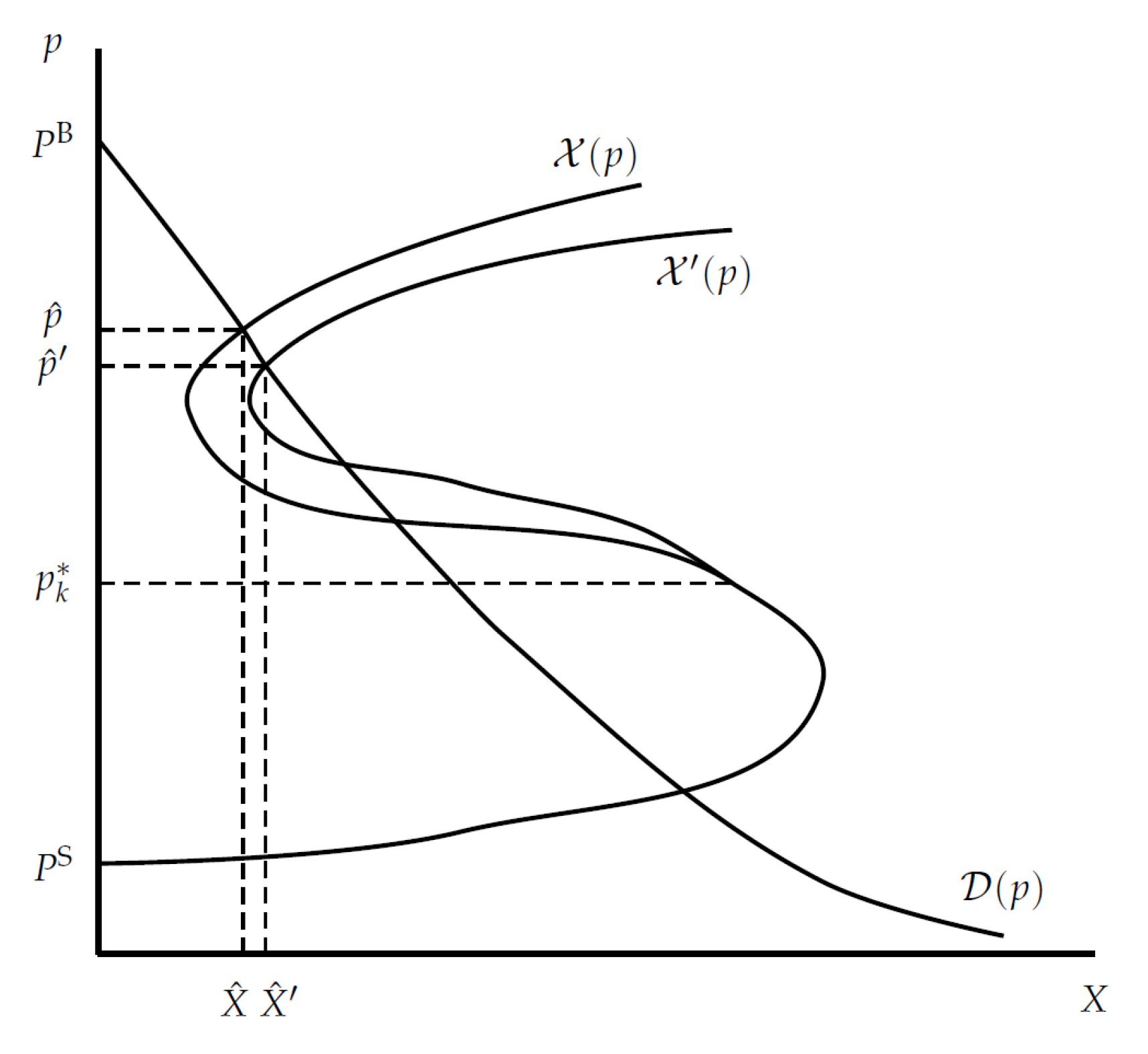
As Figure 1 illustrates and the description in Appendix A elucidates, strategic supply is a function defined only for prices above a cutoff price $P^{\mathrm{S}}$ and strategic demand is a function defined only for prices below the cutoff $P^{\mathrm{B}}$ ($P^{\mathrm{S}}$ and $P^{\mathrm{B}}$ are defined in Equations (11) and (15) respectively). Existence of a non-autarkic Nash equilibrium requires $P^{\mathrm{S}}<P^{\mathrm{B}}$, which is assumed throughout the rest of the paper. When all buyers’ preferences are binormal, strategic demand is strictly decreasing in p ([8], Lemma 5.1) but strategic supply may be non-monotonic.5 As such, multiple non-autarkic Nash equilibria may be admitted. Attention in this paper will be confined to “regular” Nash equilibria, and to changes in the environment that preserve the set of regular equilibria.6

Figure 1. The effect on equilibrium aggregates of an additional active seller.

Figure 1. The effect on equilibrium aggregates of an additional active seller.

Definition 3. A non-autarkic Nash equilibrium with price $\widehat{p}$ isregularif there is an $ϵ>0$ such that for all $p\in (\widehat{p}-ϵ,\widehat{p})$, $\mathcal{X}\left(p\right)\le \mathcal{D}\left(p\right)$ and for all $p\in (\widehat{p},\widehat{p}+ϵ)$, $\mathcal{X}\left(p\right)\ge \mathcal{D}\left(p\right)$.

If there is a unique equilibrium then it is regular. Uniqueness of equilibrium is ensured when strategic supply is non-decreasing in p, which is so when all sellers’ preferences are both binormal and everywhere satisfy ICS ([8], Lemma 5.2, where the additional restriction on sellers’ preferences is called “partial substitutes”).

At a non-autarkic Nash equilibrium with price $\widehat{p}$ the aggregate supply is $\widehat{X}=\mathcal{X}\left(\widehat{p}\right)$ and the aggregate bid is $\widehat{B}=\widehat{p}\mathcal{D}\left(\widehat{p}\right)$. Individuals’ equilibrium strategies can be found by deducing their actions consistent with a Nash equilibrium with these characteristics.

By analyzing bilateral oligopoly as two partial games, strategic supply and demand are defined independently of the set of agents on the other side of the market, the appeal of which for an analysis of the effects of entry is clear. The effect on the price and volume of trade from entry on one side of the market can be found from the change in strategic supply or demand, as appropriate. The change in individual strategies can then be determined by considering the individual actions that are consistent with the new equilibrium aggregates and the change this implies.

5. Aggregate Comparative Statics

Consider first the entry of an additional seller. When the set of sellers changes to $I^{\mathrm{S}\prime }=I^{\mathrm{S}}\cup \left\{k\right\}$ (post-change quantities are denoted with primes) nothing changes in the analysis of the buyers so the effect on the price and volume of trade can be deduced from the change in strategic supply, which increases for all prices exceeding $p_k^{*}={\partial }_k(e_k,0)$ (see Dickson and Hartley [8], Section 6.1). As inspection of Figure 1 makes clear, at any regular equilibrium where $\widehat{p}>p_k^{*}$ (in which the new seller will be active) the equilibrium volume of trade will increase and the equilibrium price will decline.7

Proposition 1. Suppose an additional seller k joins the economy that preserves the set of equilibria. Then any Nash equilibrium where $\widehat{p}\le p_k^{*}$ is unchanged. Conversely, at any regular equilibrium where $\widehat{p}>p_k^{*}$ the equilibrium price falls and the quantity of the good traded increases: ${\widehat{p}}^{\prime }<\widehat{p}$ and ${\widehat{X}}^{\prime }>\widehat{X}$.

As such, regular equilibria in bilateral oligopoly exhibit the features of quasi-competitiveness: the price reduces and the volume of trade increases when there is more supply-side competition.8

Whilst aggregate supply in the new equilibrium increases, the same conclusion cannot be drawn for the aggregate bid: strategic demand is monotonic in p, but when buyers’ preferences are only binormal the same cannot be said of the aggregate bid. The following lemma demonstrates that the conditions on preferences that govern the change in the value of individual demand in a competitive framework also govern the change in the value of aggregate demand consistent with a Nash equilibrium in bilateral oligopoly.

Lemma 2. If, in addition to being binormal, all buyers’ preferences satisfy ECD (ICD), then $\mathcal{B}\left(p^{\prime }\right)\le (>)\mathcal{B}\left(p\right)$ for any $P^{\mathrm{B}}>p^{\prime }>p>0$.

Since $p=B/X$ and p decreases in the presence of an additional seller, if B increases, its proportional increase must not exceed the proportional increase in X. Nevertheless, the aggregate bid may increase and Lemma 2 gives the conditions under which this is so.

Corollary 3. Suppose an additional seller k enters the economy. If, in addition to being binormal, all buyers’ preferences locally satisfy9 ECD (ICD), then ${\widehat{B}}^{\prime }\ge (<)\widehat{B}$ at any regular equilibrium where $\widehat{p}>p_k^{*}$.

In bilateral oligopoly the aggregate bid is the revenue shared amongst the sellers. It is useful to define the elasticity of strategic demand as

$$\eta (p,\Delta p)=-\frac{p\Delta \mathcal{D}\left(p\right)}{\mathcal{D}\left(p\right)\Delta p}$$

(1)

Since, by definition, $\mathcal{B}\left(p\right)=p\mathcal{D}\left(p\right)$, strategic demand is elastic (inelastic) if and only if $\mathcal{B}\left(p\right)$ is decreasing (increasing) in p, and so the conditions presented in Lemma 2 that govern the monotonicity of the aggregate bid also govern whether strategic demand is elastic or inelastic.

6. Individual Comparative Statics

Attention now turns to deducing the effect of the introduction of a new seller on existing traders’ strategies and payoffs by determining their actions consistent with the new equilibrium aggregates and the change this implies. To retain tractability the analysis is restricted to small changes, which can be formally justified by confining attention to a regular equilibrium in which the price is $\widehat{p}$, and the introduction of a seller k who has $p_k^{*}$ smaller than, but close to, $\widehat{p}$.10 This equilibrium is referred to as the “closest regular equilibrium”.

Looking first at the buyers, the equilibrium payoff to buyer $i\in I^{\mathrm{B}}$ is ${\widehat{u}}_i=u_i({\widehat{b}}_i/\widehat{p},m_i-{\widehat{b}}_i)$. Utilizing the first-order condition (see Expression (12) in Appendix A), the change in her payoff is

$$\begin{array}{cc}\hfill \mathrm{d}{\widehat{u}}_i& =((1/\widehat{p})u_i^1-u_i^2)\mathrm{d}{\widehat{b}}_i-({\widehat{b}}_i/{\widehat{p}}^2)u_i^1\mathrm{d}\widehat{p}\hfill \end{array}$$

$$\begin{array}{cc}& =u_i^1/\widehat{p}[({\widehat{b}}_i/\widehat{B})\mathrm{d}{\widehat{b}}_i-({\widehat{b}}_i/\widehat{p})\mathrm{d}\widehat{p}]\hfill \end{array}$$

(2)

In the presence of an additional active seller, $\mathrm{d}\widehat{p}<0$ and $\mathrm{d}\widehat{X}>0$ (Proposition 1). If all buyers are homogeneous then their payoffs necessarily increase regardless of their bid response: either all buyers increase their bid, in which case the expression above is positive; or they all reduce their bid, in which case the equilibrium payoff can be written $u_i\left(\right(1/|I^{\mathrm{B}}\left|\right)\widehat{X},m_i-{\widehat{b}}_i)$, which necessarily increases since $m_i-{\widehat{b}}_i$ increases and $\mathrm{d}\widehat{X}>0$. When buyers are heterogeneous, they may have different bid responses; however, it is transparent from (2) that if all buyers increase their bid, they will each receive a higher equilibrium payoff. The following proposition11 collects these ideas.

Proposition 4. Suppose an additional seller enters the economy. Then if either (a) all buyers’ preferences are not only binormal but also locally satisfy ECD or (b) all buyers are homogeneous, all buyers at the closest regular equilibrium are made strictly better off.

With a heterogeneous buyer set and some buyers whose preferences satisfy ICD, there may be buyers that optimally reduce their bid and suffer a lower level of equilibrium utility. Note, however, that even if all buyers reduce their bid, not all buyers can be made worse off: they will retain more money and their allocation of the good is $({\widehat{b}}_i/\widehat{B})\widehat{X}$, which cannot decrease for all buyers since $\mathrm{d}\widehat{X}>0$ and ${\sum }_{j\in I^{\mathrm{B}}}{\widehat{b}}_j/\widehat{B}=1$.

Corollary 5. Any regular Nash equilibrium in the presence of an additional seller cannot be Pareto inferior to the corresponding Nash equilibrium in the original economy.

Turning now to the supply side, the equilibrium payoff of seller $i\in I^{\mathrm{S}}$ is given by ${\widehat{u}}_i=u_i(e_i-{\widehat{x}}_i,{\widehat{x}}_i\widehat{p})$. The change in her payoff is

$$\begin{array}{cc}\hfill \mathrm{d}{\widehat{u}}_i& =(-u_i^1+\widehat{p}{u}_i^2)\mathrm{d}{\widehat{x}}_i+{\widehat{x}}_i{u}_i^2\mathrm{d}\widehat{p}\hfill \end{array}$$

$$\begin{array}{cc}& =u_i^2[({\widehat{x}}_i/\widehat{X})\widehat{p}\mathrm{d}{\widehat{x}}_i+{\widehat{x}}_i\mathrm{d}\widehat{p}]\hfill \end{array}$$

(3)

(Expression (8) in Appendix A gives the first-order condition used in the second line.)

The presence of an additional active seller lowers the equilibrium price, so if sellers reduce their supply, they will receive a lower equilibrium payoff and the conventional wisdom applies. Conversely, if a seller optimally increases her supply, her payoff may increase.

To explore the conditions under which this occurs, recall that sellers can be thought of as engaging in a contest in which the aggregate bid is shared in proportion to supply to the market. In the presence of an additional seller the contest is more competitive, but the size of the prize being contested may differ. How much a seller should supply in this contest relative to her previous supply will depend on the conjectured change in the aggregate bid in relation to the additional competitiveness of the contest, and this hinges crucially on the elasticity of strategic demand defined12 in (1), as the following lemma demonstrates.

Lemma 6. When an additional seller enters the economy the change in supply of an existing seller $i\in I^{\mathrm{S}}$ at the closest regular equilibrium satisfies

$$\mathrm{d}{\widehat{x}}_i>(=,<)0\iff \eta \left(\widehat{p}\right)>(=,<)\frac{-\frac{1}{\widehat{p}}\left({\widehat{y}}_2\frac{\partial {\partial }_i\left(\widehat{y}\right)}{\partial y_2}-{\partial }_i\left(\widehat{y}\right)\right)}{{\widehat{x}}_i/\widehat{X}}:={\tilde{\eta }}_i$$

(4)

Since buyers’ preferences are binormal, $\eta \left(\widehat{p}\right)>0$. As such, if a seller’s preferences satisfy DCS, (4) implies she will always increase her supply; such sellers have a strong preference to preserve their money holdings, which, since the price reduces, requires supply to increase. A seller whose preferences satisfy ICS (with a strict inequality) may either increase or reduce supply: her supply will increase if the elasticity of strategic demand exceeds a certain threshold that is inversely related to her market share (and also depends on her preferences), implying that supply only increases in the more competitive contest if the size of the prize does not reduce too much. Notice that, other things equal, the critical value of the elasticity is lower for sellers with a larger market share: smaller sellers might reduce their supply at the same time as larger sellers increase supply.

It is instructive to consider the special case where sellers are modeled as profit-maximizing firms.13 In this case the condition for the elasticity in Expression (4) becomes $\eta \left(\widehat{p}\right)>(=,<)\frac{1}{{\widehat{x}}_i/\widehat{X}}-1$, so for sellers that are not “dominant” (i.e., have market share less than 50%) to increase supply, the aggregate bid must increase (i.e., strategic demand must be elastic), and increase by a sufficient amount that is larger for sellers with smaller market share. If strategic demand is inelastic and there are no dominant firms, then according to Lemma 6 all firms will reduce their supply and (3) can be used to deduce when the conventional wisdom applies.

Corollary 7. Suppose the preferences of all buyers are both binormal and locally satisfy ICD, and that sellers are profit-maximizing firms, none of which are dominant. Then when an additional firm enters the economy, existing firms reduce their supply and their equilibrium profit declines.

When strategic demand is not too inelastic and there are sellers whose share of the market is not too small, these sellers may optimally increase supply in the presence of an additional seller. As noted, increasing supply is only a necessary condition for a seller’s payoff to increase; the sufficient condition is presented in the next proposition.

Proposition 8 When an additional seller enters the economy, the payoff of seller $i\in I^{\mathrm{S}}$ at the closest regular equilibrium increases (remains constant, decreases) if and only if

$$\eta \left(\widehat{p}\right)>(=,<){\tilde{\eta }}_i+\frac{1}{{\widehat{x}}_i/\widehat{X}}\frac{\widehat{X}}{\widehat{p}}{\widehat{\phi }}_i:={\overline{\eta }}_i$$

(5)

where ${\tilde{\eta }}_i$ is defined in (4) and, for $i\in I^{\mathrm{S}}$, ${\widehat{\phi }}_i:=-\frac{\partial {\partial }_i\left(\widehat{y}\right)}{\partial y_1}+\widehat{p}\frac{\partial {\partial }_i\left(\widehat{y}\right)}{\partial y_2}+\frac{\widehat{p}}{\widehat{X}}$, which is strictly positive when preferences are binormal.

For a seller to increase supply, the elasticity of strategic demand must exceed ${\tilde{\eta }}_i$. For her payoff to increase, it must exceed a higher threshold again related inversely to her market share and also to preferences. The aggregate bid from the buyers must increase by an amount that ensures the seller’s allocation of money increases and that the gain in utility from this more than outweighs the reduction in utility from lower final holdings of the good after increasing supply. When sellers are modeled as profit-maximizing firms ${\overline{\eta }}_i={\tilde{\eta }}_i+\frac{1}{{\widehat{x}}_i/\widehat{X}}(1+(\widehat{X}/\widehat{p})C_i^{\prime \prime }\left({\widehat{x}}_i\right))$ and a firm’s profit will increase when strategic demand is sufficiently elastic, the firm has a large enough market share and its rate of increase in marginal cost is not too high: when the firm increases supply in competing for its share of the total revenue, for profit to increase its allocation of that revenue must increase by more than the increased cost of production.

Notice that in a given entry scenario it might be the case that some sellers suffer a reduction in payoff whilst others benefit from the change; if so it will be those sellers with a relatively large market share that will benefit. Contrary to the substantial literature on entry deterrence, in thin bilateral oligopoly environments in which strategic demand is sufficiently elastic there may be sellers that encourage the entry of additional sellers to the market.

Whilst there may be market conditions in which entry by additional active sellers is encouraged by at least some existing sellers, when all sellers’ preferences everywhere satisfy ICS, successive entry will eventually lead to the payoffs of incumbents decreasing with further entry, implying that in large economies the conventional wisdom applies. This can be deduced by the following reasoning. First, each seller’s market share decreases as new active sellers enter the economy.14 Since the threshold that the elasticity of strategic demand must exceed for a seller to enjoy a higher payoff in the presence of new entrants (see (5)) is inversely related to that seller’s market share, this means that with successive entry, strategic demand must be increasingly elastic for payoff-increasing competition to be preserved. Whilst, when moving “down” the strictly decreasing strategic demand curve (as is the case when additional sellers enter the economy) elasticity may temporarily increase, this cannot be so globally. Thus, for a given set of buyers (i.e., a given strategic demand function) there will be a critical density of sellers beyond which all sellers’ payoffs will fall with the entry of additional sellers: when the economy is “large enough” the conventional wisdom applies.15

7. Example Revisited

To illustrate the main points of the analysis, a more general form of the example from Section 3 will be considered. There are $m\ge 2$ buyers each of which has an endowment of two units of money and preferences given by $u\left(y\right)=\alpha y_1-\frac{\gamma }{2}{y}_1^2+y_2$, and $n\ge 2$ sellers with quadratic costs given by $C\left(x\right)=\beta x+\frac{\mu }{2}{x}^2$. The arguments in Appendix A can be used to deduce that strategic supply takes the form $\mathcal{X}\left(p\right)=-\frac{n\beta }{\mu }+\frac{n-1}{\mu }p$ with $P^{\mathrm{S}}=\frac{n}{n-1}\beta$, and strategic demand takes the form $\mathcal{D}\left(p\right)=\frac{m\alpha }{\gamma }-\frac{m^2}{(m-1)\gamma }p$ with $P^{\mathrm{B}}=\frac{m-1}{m}\alpha$ (both linear). Supposing that $P^{\mathrm{S}}=\frac{n}{n-1}\beta <\frac{m-1}{m}\alpha =P^{\mathrm{B}}$ (so that a non-autarkic Nash equilibrium exists) the equilibrium price is $\widehat{p}=\frac{(m-1)(m\alpha \mu +n\beta \gamma )}{(m-1)(n-1)\gamma +m^2\mu }$ and the equilibrium volume of trade is $\widehat{X}=\frac{m\left(\right(m-1\left)\right(n-1)\alpha -mn\beta )}{(m-1)(n-1)\gamma +m^2\mu }$.

Set $m=4$, $\alpha =3$, $\beta =1/2$ and $\mu =5$ (as in the example of Section 3), leaving γ, the buyers’ preference parameter and n, the number of sellers, as free parameters. In this case $\widehat{p}=\frac{360+3n\gamma }{160+6(n-1)\gamma }$ and $\widehat{X}=\frac{4(7n-9)}{80+3(n-1)\gamma }$; the former is decreasing in n whilst the latter is increasing in n for any $\gamma >0$ (quasi-competitiveness).

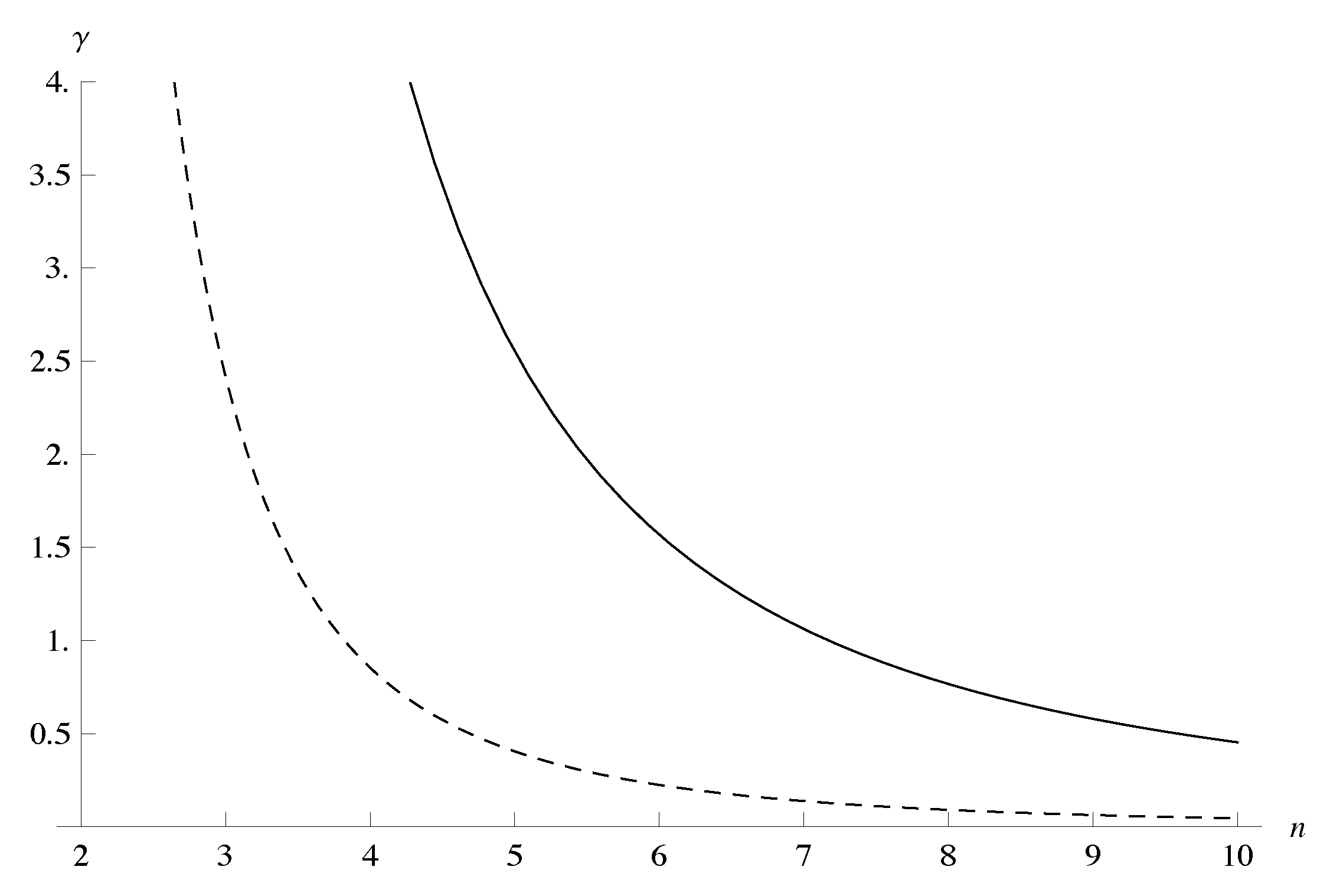
Whether firms increase supply in the presence of new firms and enjoy increased profit depends on the magnitude of the elasticity of strategic demand, which in this example is $\eta \left(\widehat{p}\right)=\frac{2(120+n\gamma )}{\gamma (7n-9)}$ (decreasing in both n and γ). Figure 2 plots the combinations of γ and n where (a) the elasticity is such that condition (4) is satisfied with equality (the solid curve) and (b) the elasticity is such that condition (5) is satisfied with equality (the dashed curve). To the south-west of these curves (i.e., for smaller n and/or γ) the conditions are satisfied with a > inequality. Thus, to the south-west of the dashed curve profit-increasing competition is observed. For any γ that is small enough profit-increasing competition will be observed for small n, but there is a critical number of firms beyond which the conventional wisdom applies.

Figure 2. Combinations of γ and n for which condition (4) is satisfied with equality (solid) and condition (5) is satisfied with equality (dashed). To the south-west of these curves the conditions hold with a > inequality, so to the south-west of the dashed curve profit-increasing competition is observed.

Figure 2. Combinations of γ and n for which condition (4) is satisfied with equality (solid) and condition (5) is satisfied with equality (dashed). To the south-west of these curves the conditions hold with a > inequality, so to the south-west of the dashed curve profit-increasing competition is observed.

8. Entry of Buyers

Similar results to those derived for entry of additional sellers apply if the number of buyers increases (with a fixed set of sellers). Since the analysis closely parallels that previously elucidated, the details are omitted. If an additional buyer l enters the economy, then strategic demand increases for all $p<p_l^{*}$. As such, at any regular equilibrium where $\widehat{p}<p_l^{*}$, it follows that ${\widehat{X}}^{\prime }\ge \widehat{X}$ and ${\widehat{p}}^{\prime }>\widehat{p}$, and consequently that ${\widehat{B}}^{\prime }>\widehat{B}$ (since $B=pX$). Analogous to Proposition 4, if all sellers’ preferences are binormal and satisfy ICS (or all sellers are homogeneous) then each seller’s supply will not reduce and their equilibrium payoffs will increase. With entry of additional sellers, the effect on the payoffs of existing sellers was governed by the change in the size of the prize they contested (the aggregate bid), measured by the elasticity of strategic demand. The prize shared by the buyers is the aggregate supply, so the effect on existing buyers’ equilibrium bids and payoffs with the entry of additional buyers is determined by the magnitude of $\xi \left(p\right):={lim}_{\Delta p\to 0}\frac{\Delta \mathcal{X}\left(p\right)}{\Delta p}$, the slope of strategic supply.16 Using deductions analogous to those in Lemma 6 and Proposition 8 (and utilizing Expressions (18) and (19)) it can be shown that for an existing buyer $i\in I^{\mathrm{B}}$

$$\mathrm{d}{\widehat{b}}_i>(=,<)0\iff \xi \left(\widehat{p}\right)>(=,<)\frac{\widehat{B}}{\widehat{p}}\left(\frac{\frac{1}{\widehat{p}}\left({\widehat{y}}_1\frac{\partial {\partial }_i\left(\widehat{y}\right)}{\partial y_1}+{\partial }_i\left(\widehat{y}\right)\right){\left(1-\frac{{\widehat{b}}_i}{\widehat{B}}\right)}^2}{\frac{{\widehat{b}}_i}{\widehat{B}}}-1\right):={\tilde{\xi }}_i$$

(6)

and their payoff increases (remains constant, decreases) if and only if

$$\xi \left(\widehat{p}\right)>(=,<){\tilde{\xi }}_i+\frac{({\widehat{b}}_i/\widehat{p}){(1-{\widehat{b}}_i/\widehat{B})}^2\left|{\widehat{\phi }}_i\right|}{{({\widehat{b}}_i/\widehat{B})}^2(\widehat{p}/\widehat{B})}:={\overline{\xi }}_i$$

(7)

where, for $i\in I^{\mathrm{B}}$, ${\widehat{\phi }}_i:=\frac{1}{\widehat{p}}\frac{\partial {\partial }_i\left(\widehat{y}\right)}{\partial y_1}-\frac{\partial {\partial }_i\left(\widehat{y}\right)}{\partial y_2}-\frac{\widehat{p}/\widehat{B}}{{(1-{\widehat{b}}_i/\widehat{B})}^2}$, which is strictly negative when preferences are binormal.

Finally, suppose there is entry to both sides of the market (attention here is focused on equilibrium aggregates). Consider a regular equilibrium with price $\widehat{p}$ and suppose an additional seller k with $p_k^{*}<\widehat{p}$ and an additional buyer l with $p_l^{*}>\widehat{p}$ join the economy (and that the set of equilibria is preserved). Since strategic supply and demand are constructed independently of the details of the other side of the market, it follows that the conclusions for the entry of sellers and buyers separately can be applied to deduce the change in strategic supply and demand functions: strategic supply increases for prices exceeding $p_k^{*}$ and strategic demand increases for prices below $p_l^{*}$. Since strategic demand is decreasing in p, it is easily deduced by visual inspection of Figure 1 that ${\widehat{X}}^{\prime }>\widehat{X}$. To determine the effect on the equilibrium aggregate bid, there are two cases to consider: (a) if ${\widehat{p}}^{\prime }\ge \widehat{p}$ then since $\widehat{B}=\widehat{p}\widehat{X}$ it is immediate that ${\widehat{B}}^{\prime }>\widehat{B}$; (b) if ${\widehat{p}}^{\prime }<\widehat{p}$ then a relatively straightforward modification of Lemma 2 (which demonstrated that for a given set of buyers $\mathcal{B}\left(p\right)$ is decreasing in p if all buyers’ preferences satisfy ECD) implies that under the same conditions on preferences the aggregate bid in the presence of an additional buyer will also be higher. This allows the conclusion in the following proposition.

Proposition 9. Suppose the preferences of all buyers are both binormal and locally satisfy ECD. Then when an additional buyer and seller enter the economy, both the aggregate supply and the aggregate bid increase at any regular equilibrium with $p_k^{*}<\widehat{p}<p_l^{*}$.17

If all sellers’ preferences everywhere satisfy ICS, then strategic supply is non-decreasing and the conclusions of Proposition 9 apply to the unique non-autarkic Nash equilibrium. If all buyers’ preferences everywhere satisfy ECD, the conclusions apply under arbitrary expansion of the set of traders. Amir and Bloch [9] (Proposition 3) demonstrate that aggregate offers and bids monotonically increase under replication of the economy but require the arguably strong gross substitutes condition to hold for all traders (i.e., all traders’ preferences satisfy strict versions of both ICS and ECD). Proposition 9 thus represents a substantial weakening of the assumptions required for monotonicity of the aggregate bid and aggregate supply under entry to both sides of the market, and therefore for monotonic convergence of equilibrium aggregates along an appropriate replication sequence.

9. Conclusions

By exploiting the aggregative structure of the strategic market game, it has been possible to undertake a comprehensive study of the effects of entry in bilateral oligopoly without making any assumptions that restrict the heterogeneity of traders or imposing overly restrictive assumptions on their payoffs. As well as considering entry on both sides of the market, entry to each side of the market in turn was studied. It was found that bilateral oligopoly is quasi-competitive (the volume of trade increases, and the price reduces when additional sellers enter and increases when additional buyers enter), and that the payoffs of traders on the same side of the market to the entrant can increase so long as traders on the other side of the market sufficiently increase their market strategies. In particular, with increased supply-side competition, if the elasticity of demand exceeds a threshold that is inversely related to a seller’s market share, that seller will enjoy a higher pay-off at the new equilibrium. Likewise, with increased demand-side competition, a buyer can be made better off if the slope of strategic supply exceeds a threshold that is inversely related to her market share. This raises the possibility that in markets with few participants, incumbents with sufficiently large market shares may encourage new entrants to their side of the market, in contrast to the extensive literature on entry deterrence.

References

- Frank, C., Jr. Entry in a Cournot market. Rev. Econ. Stud. 1965, 32, 245–250. [Google Scholar] [CrossRef]
- Ruffin, R. Cournot oligopoly and competitive behavior. Rev. Econ. Stud. 1971, 38, 493–502. [Google Scholar] [CrossRef]
- Okuguchi, K. Quasi-competitiveness and Cournot oligopoly. Rev. Econ. Stud. 1973, 40, 145–148. [Google Scholar] [CrossRef]
- Seade, J. On the effects of entry. Econometrica 1980, 48, 479–489. [Google Scholar] [CrossRef]
- Amir, R.; Lambson, V. On the effects if entry in Cournot markets. Rev. Econ. Stud. 2000, 67, 235–254. [Google Scholar] [CrossRef]
- Bloch, F.; Ghosal, S. Stable trading structures in bilateral oligopolies. J. Econ. Theory 1997, 74, 368–384. [Google Scholar] [CrossRef]
- Groh, C. Sequential Moves and Comparative Statics in Strategic Market Games; Department of Economics, University of Mannheim: Mannheim, Germany, 1999. [Google Scholar]
- Dickson, A.; Hartley, R. The strategic Marshallian cross. Games Econ. Behav. 2008, 64, 514–532. [Google Scholar] [CrossRef]
- Amir, R.; Bloch, F. Comparative statics in a simple class of strategic market games. Games Econ. Behav. 2009, 65, 7–24. [Google Scholar] [CrossRef]
- Novshek, W. On the existence of Cournot equilibrium. Rev. Econ. Stud. 1985, 52, 85–98. [Google Scholar] [CrossRef]
- Cornes, R.; Hartley, R. Asymmetric contests with general technologies. Econ. Theory 2005, 26, 923–946. [Google Scholar] [CrossRef]
- Corchón, L. Comparative statics for aggregative games: The strong concavity case. Math. Soc. Sci. 1994, 28, 151–165. [Google Scholar] [CrossRef]
- Jensen, M. Aggregative games and best reply potentials. Econ. Theory 2010, 43, 45–66. [Google Scholar] [CrossRef]
- Gabszewicz, J.J.; Michel, P. Oligopoly Equilibrium in Exchange Economies. In Trade, Technology and Economics: Essays in Honor of Richard G. Lipsey; Eaton, B., Harris, R., Eds.; Elgar: Cheltenham, UK, 1997; pp. 217–240. [Google Scholar]
- Shapley, L.; Shubik, M. Trade using one commodity as a means of payment. J. Polit. Econ. 1977, 85, 937–968. [Google Scholar] [CrossRef]
- 1.A game is aggregative when each player’s payoff can be expressed as a function of their own strategy and the aggregate of all players’ strategies. This structure can be exploited in the analysis of the game enabling techniques that differ from standard best response analysis to be used in studying equilibrium that avoid using many-dimensional fixed-point theorems, even with heterogeneous players. See, for example, Novshek [10] for an application to Cournot competition, Cornes and Hartley [11] for an application to contests and Corchón [12] and Jensen [13] for treatments of general aggregative games.
- 2.The competitive first-order condition is , implicit differentiation of which reveals when preferences are binormal. Thus, competitive supply is increasing (decreasing) if and only if is decreasing (increasing) in .
- 3.When preferences are binormal, whether competitive demand is elastic or inelastic depends on whether is increasing or decreasing in . To see this, write the competitive first-order condition as ; implicit differentiation yields and demand is elastic (unit elastic, inelastic) when . (Due to the weak inequality ECD allows for unit-elastic demand.)
- 4.Each partial game, with an appropriate change of variables, is strategically equivalent to a Tullock contest. Cornes and Hartley [11] have studied equilibria in such games by exploiting their aggregative properties.
- 5.The asymmetry arises because the analysis is of transactions of the good denominated in units of commodity money: like , is non-monotonic when preferences are only binormal but is.
- 6.This is done to retain tractability of changes in individuals’ payoffs, which is the focus of the paper. Some deductions can be made for aggregates at extremal equilibria even if the set of equilibria is not preserved; see Dickson and Hartley [8] (Section 6.3) for some discussion of this.
- 7.Amir and Bloch [9] (Propositions 1 and 2 and Claims 1 and 2) draw similar conclusions for the extremal aggregate bid and price when buyers enter, although the conclusions for the change in price rely on traders being homogeneous.
- 8.For any arbitrary expansion of the set of sellers, the same conclusion can be drawn for regular equilibria at which .
- 9.The additional conditions on preferences need only be satisfied in a sufficiently large neighborhood of the original equilibrium in question.
- 10.In the spirit of an analysis that exploits the aggregative properties of the game, this approach is preferred to assuming traders are homogeneous and differentiating equilibrium expressions with respect to the number of traders.
- 11.Amir and Bloch [9] (Proposition 1) conclude that when traders are homogeneous and preferences are binormal, the payoffs of traders on the opposite side of the market to the entrant increase. This proposition (and its analog when new buyers enter) generalizes this result to the case of heterogeneous traders, but stronger assumptions than binormality are required (which need only be satisfied in a sufficiently large neighborhood of the original equilibrium).
- 12. is, with a slight abuse of notation, the elasticity of strategic demand when infinitesimal changes are considered where, if necessary, the appropriate one-sided derivative is used (in this case as ).
- 13.See the Remark in Section 2 and recall that in this case all sellers’ preferences everywhere satisfy ICS, implying the equilibrium is unique.
- 14.This is obvious when sellers are homogeneous. When the set of sellers is heterogeneous each seller’s share of the total supply that is consistent with a Nash equilibrium in which the price and aggregate supply take particular values, denoted —see Appendix A—is strictly decreasing in X and increasing in p when preferences satisfy ICS. Thus, for and , as is the case when a new active seller enters the market, each existing seller’s equilibrium market share will decline.
- 15.If there are homogeneous sellers modeled as firms with constant marginal costs the conventional wisdom holds when .
- 16.If necessary, the appropriate one-sided derivative should be used in defining , which in this case is as .
- 17.As with entry to one side of the market, this extends to arbitrary expansion of the sets of buyers and sellers and regular equilibria where (the set of which should be preserved).
- 18.When sellers are modeled as profit-maximizing firms, the analysis is the same when costs are strictly convex but with . When firms have constant marginal costs (say ), then , so strategic supply is perfectly elastic at and is otherwise undefined. In the presence of an additional buyer, the analysis parallels that in the text except the price remains constant. The analysis of entry to the supply side remains the same so long as the new firm has (as is the case with homogeneous firms).
- 19.Recall that when preferences are binormal and , implying .
© 2013 by the author; licensee MDPI, Basel, Switzerland. This article is an open access article distributed under the terms and conditions of the Creative Commons Attribution license (http://creativecommons.org/licenses/by/3.0/).
Share and Cite
MDPI and ACS Style
Dickson, A. The Effects of Entry in Bilateral Oligopoly. Games 2013, 4, 283-303. https://doi.org/10.3390/g4030283
AMA Style
Dickson A. The Effects of Entry in Bilateral Oligopoly. Games. 2013; 4(3):283-303. https://doi.org/10.3390/g4030283
Chicago/Turabian StyleDickson, Alex. 2013. "The Effects of Entry in Bilateral Oligopoly" Games 4, no. 3: 283-303. https://doi.org/10.3390/g4030283