A Choice Prediction Competition for Social Preferences in Simple Extensive Form Games: An Introduction

Abstract

Two independent, but related, choice prediction competitions are organized that focus on behavior in simple two-person extensive form games ( http://sites.google.com/site/extformpredcomp/): one focuses on predicting the choices of the first mover and the other on predicting the choices of the second mover. The competitions are based on an estimation experiment and a competition experiment. The two experiments use the same methods and subject pool, and examine games randomly selected from the same distribution. The current introductory paper presents the results of the estimation experiment, and clarifies the descriptive value of some baseline models. The best baseline model assumes that each choice is made based on one of several rules. The rules include: rational choice, level-1 reasoning, an attempt to maximize joint payoff, and an attempt to increase fairness. The probability of using the different rules is assumed to be stable over games. The estimated parameters imply that the most popular rule is rational choice; it is used in about half the cases. To participate in the competitions, researchers are asked to email the organizers models (implemented in computer programs) that read the incentive structure as input, and derive the predicted behavior as an output. The submission deadline is 1 December 2011, the results of the competition experiment will not be revealed until that date. The submitted models will be ranked based on their prediction error. The winners of the competitions will be invited to write a paper that describes their model.

1. Introduction

Experimental studies of simple social interactions reveal robust behavioral deviations from the predictions of the rational economic model. People appear to be less selfish, and less sophisticated than the assumed Homo Economicus. The main deviations from rational choice (see a summary in

Table 1. Sequential two-player games that show deviations from rationality.1

Game	Description	Rational prediction	Main findings
Ultimatum [9]	A Proposer offers an allocation of a pie (e.g., $10) between herself and a responder. If the responder accepts the offer, the money is allocated. If she rejects, both get nothing	The responder maximizes own payoff thus agrees to any allocation. The proposer, anticipating that, offers the lowest amount possible to the responder	Most proposers suggest equal split when such split is possible. Low offers (below 30% of the pie) are typically rejected. [9]
Dictator [10]	A “Dictator” determines an allocation of an endowment (e.g., $10) between herself and a recipient	The dictator, maximizing their own payoff, gives $0 to the recipient	Dictators, on average, give 30% of the endowment. [10]
Trust [11]	A sender receives an endowment (e.g., $10) and can send any proportion of it to the responder. The amount sent is multiplied (e.g., by 3). The responder then decides how much to send back.	Responder maximizes their own payoff and thus sends back $0. The sender, anticipating that, sends $0.	Most senders send half or more of their endowment. Many responders (e.g., 44% in [11]) return at least the amount sent.
Gift exchange [12]	A “manager” (M) determines a wage (w) to “hire” an “employee”(E). The employee then choose an effort level e which is costly (c(e)). The profit functions are:	The employee chooses minimum effort. Anticipating that, the manager chooses the minimum wage.	The minority of transactions (less than 9%) involve minimal wages and effort. About 2/3 of the managers offers are higher than 50. [12]

) can be described as the product of a small set of psychological factors. Those factors include (i) altruism or warm glow [1]; (ii) envy or spitefulness [2]; (iii) inequality aversion [3,4]; (iv) reciprocity [5,6]; (v) maximizing joint payoff [7]; (vi) competitiveness [7]; and (vii) level-k reasoning [8].

Recent research demonstrates the potential of simple models that capture these psychological factors e.g., [3,5,13]. However, there is little agreement concerning the best abstraction and the relative importance of the distinct psychological factors. The main goal of the current project is to address the quantitative “best abstractions and relative importance” questions with the organization of a choice prediction competition. It focuses on simple response games, similar by structure to the games studied by Charness and Rabin [14]. The game structure, presented in Figure 1, involves two players acting sequentially. The first mover (Player 1) chooses between action Out, which enforces an “outside option” payoffs on the two players (f1 and s1 for Players 1 and 2 respectively), and action In. If In is chosen then the responder (Player 2) determines the allocation of payoffs by choosing between actions Left that yields the payoffs f2, s2, and action Right that yields the payoffs f3, s3.

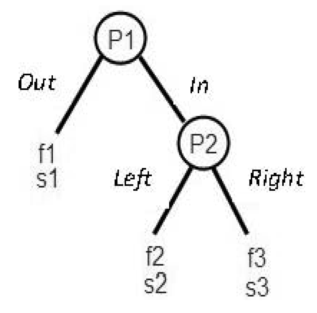
The selected structure has two main advantages: the first is that, depending on the relation between the different payoffs, this structure allows for studying games that are similar to the famous examples considered in Table 1 (ultimatum, trust etc.), and at the same time allows for expanding the set of game-types. Secondly, although this structure is simple, it is sufficient to reproduce the main deviations from rational choice considered by previous studies. For example, both players can exhibit their preferences over different outcome distributions between themselves and the other player. In addition, the “opting out” feature of the game can color action In by Player 1 as a selfish, altruistic, or neutral act (depending on the payoffs), allowing for reciprocal behavior by Player 2 (punishing or rewarding Player 1′s decision). These properties make the current set of games a natural test case for models of social preferences.

Figure 2 presents a classification of the space of games implied by Figure 1′s game structure. The classification is based on the relation between the different payoffs for each player in a specific class of games. It provides a closer look into the potential conflicts that may be involved in each game, as well as clarifying the game's likelihood of occurrence under a random selection from that space. The classification reveals that only a small proportion of the games in Figure 2′s space are similar to the games that have been extensively used by previous studies. For example, ultimatum-like games, special cases of the costly punishment (c.p.) type of games in which f1 = s1, capture less than 1% of the entire space of possible games. Similarly, the likelihood that a trust-like game would be randomly sampled from the space is only about 4%. The most likely games are typically less interesting than the famous examples: a large proportion of games include a “common interest” option that maximizes both player's payoffs, and many other games are “safe shot” games for Player 1 as the payoff from In is higher than that of Out independently of Player 2′s choice.

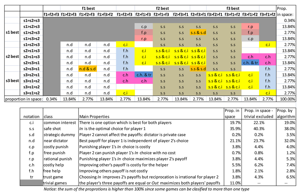
The current study focuses on games that were sampled from Figure 2′s space using the quasi random sampling algorithm described in Appendix 1. The algorithm excludes the sampling from the trivial class (games in which action Out yields the best payoff for both players or in which all payoffs are equal for a player—the dark gray cells) and implies slight oversampling of interesting games. The implied sampling proportions by this algorithm are presented on the rightmost column in the lower panel of Figure 2.

The Structure of the Competition and the Problem Selection Algorithm

The current paper introduces two independent but related competitions: one for predicting the proportion of In choices by Player 1, and the other for predicting the proportion of Right choices by Player 2. Both competitions focus on the same games, and are based on two experiments: An “estimation” and a “competition” experiment.2 We describe the first experiment (and several baseline models) below, and challenge other researchers to predict the results of the second experiment. The competition criteria are described in Section 4. The two experiments examine different games and different participants, but use the same procedure, and sample the games and the participants from the same space.

Each experiment includes 120 games. The six parameters that define each game (the payoffs f1–f3, and s1–s3, see Figure 1) were selected using the algorithm presented in Appendix 1. The algorithm implies a nearly uniform distribution of each parameter in the range between −$8 and + $8. The 120 games studied in the estimation experiment are presented in Table 1.

2. Experimental Method

The estimation experiment was run in the CLER lab at Harvard. One hundred and sixteen students participated in the study, which was run in four independent sessions, each of which included between 26 and 30 participants. Each session focused on 60 of the 120 extensive form games presented in

Table 2. The 120 games studied in the estimation experiment ranked by the Mean Squared Deviation from the Subgame Perfect Equilibrium prediction. The left-hand columns present the payoffs of the 120 games, the right-hand columns present the experimental results (proportions of In and Right choices), the subgame perfect equilibrium predictions for these choices (SPE), and the average MSD (over the two players) between the predictions and the results.

Rank	Game	f1	s1	f2	s2	f3	s3	P(In)	P(Right)	P(In) SPE	P(Right) SPE	MSD
1	16	0	8	1	−6	−6	3	0	1	0	1	0
2	18	3	−4	−2	8	3	−5	0	0	0	0	0
3	31	−6	−6	2	−3	1	2	1	1	1	1	0
4	43	−7	1	6	4	0	−6	1	0	1	0	0
5	49	5	−2	4	−5	−3	5	0	1	0	1	0
6	56	0	−2	8	3	7	−7	1	0	1	0	0
7	63	5	3	−3	6	0	8	0	1	0	1	0
8	70	−6	−6	0	8	−1	−6	1	0	1	0	0
9	84	−4	1	1	−8	8	0	1	1	1	1	0
10	86	−5	1	0	−6	−4	−4	1	1	1	1	0
11	90	−4	−4	0	−7	7	−4	1	1	1	1	0
12	93	2	4	−7	7	3	−5	0	0	0	0	0
13	97	0	6	3	−7	6	−2	1	1	1	1	0
14	105	8	−5	−6	−5	−3	6	0	1	0	1	0
15	111	−5	6	4	−4	5	4	1	1	1	1	0
16	117	−3	−6	8	0	7	3	1	1	1	1	0
17	35	0	1	6	1	8	−6	1	0.03	1	0	0
18	39	5	7	7	−7	0	4	0.03	1	0	1	0
19	46	−4	−2	7	6	−4	3	1	0.03	1	0	0
20	3	−7	−4	−5	8	−5	8	1	0.47	1	0.5	0
21	4	−3	−4	−1	4	3	7	1	0.97	1	1	0
22	30	2	−8	7	−1	6	−7	0.97	0	1	0	0
23	36	−5	3	7	−7	−4	5	1	0.97	1	1	0
24	37	−6	1	−2	−6	1	−3	1	0.97	1	1	0
25	44	−7	6	−5	2	−4	7	1	0.97	1	1	0
26	79	0	0	−5	5	−1	−6	0.04	0	0	0	0
27	89	6	−7	−3	−3	6	−7	0.04	0	0	0	0
28	91	2	−6	−7	−1	0	−6	0.04	0	0	0	0
29	96	2	6	−3	6	3	−3	0	0.04	0	0	0
30	66	−6	−2	1	−4	−4	−4	0.96	0.5	1	0.5	0
31	81	−6	−5	0	−1	−4	−6	0.96	0	1	0	0
32	82	0	8	6	5	8	3	0.96	0	1	0	0
33	83	−6	−6	−1	−1	5	−5	0.96	0	1	0	0
34	103	−7	−5	−5	5	−6	−3	0.96	0	1	0	0
35	104	−5	−4	4	−7	2	2	1	0.96	1	1	0
36	26	−1	4	1	0	5	−2	0.97	0.03	1	0	0
37	23	−3	−5	3	−3	6	−1	0.97	0.97	1	1	0
38	53	−6	2	−7	−2	0	2	0.97	0.97	1	1	0
39	67	−3	−1	−5	−3	6	0	0.96	0.96	1	1	0
40	101	2	−6	7	−8	6	−6	0.96	0.96	1	1	0
41	25	−7	1	−6	1	0	3	1	0.93	1	1	0
42	32	−3	6	2	−4	5	−3	1	0.93	1	1	0
43	87	3	−2	2	0	6	3	0.93	1	1	1	0
44	106	4	−1	6	3	0	−2	0.93	0	1	0	0
45	10	−2	5	−4	7	−2	−2	0.07	0	0	0	0
46	24	2	−4	−3	5	3	−2	0	0.07	0	0	0
47	55	6	0	−5	4	0	−2	0	0.07	0	0	0
48	12	2	−7	3	3	4	−6	0.93	0.03	1	0	0
49	15	1	−4	1	2	6	5	0.93	0.97	1	1	0
50	59	−6	5	2	0	7	−8	0.97	0.07	1	0	0
51	120	−2	−7	−3	−6	0	3	0.96	0.93	1	1	0
52	64	6	−2	1	1	4	−3	0.07	0.04	0	0	0
53	102	−1	−6	−4	−2	−4	−3	0.07	0.04	0	0	0
54	62	2	−6	3	−2	−4	5	0.07	0.96	0	1	0
55	99	−5	7	−2	−1	4	−4	0.96	0.07	1	0	0
56	114	−4	1	−3	6	6	1	0.96	0.07	1	0	0
57	118	−5	−6	7	7	4	−6	0.96	0.07	1	0	0
58	11	−2	1	5	−7	5	−7	0.93	0.43	1	0.5	0
59	58	−6	0	−1	−5	−6	−7	0.93	0.07	1	0	0
60	60	−8	3	6	4	−3	−2	0.93	0.07	1	0	0
61	13	5	−6	0	1	1	−7	0.07	0.07	0	0	0
62	29	0	1	−2	5	5	−5	0.1	0.03	0	0	0.01
63	71	7	−1	5	4	−5	7	0.04	0.89	0	1	0.01
64	107	4	−3	5	−7	2	−3	0.11	0.96	0	1	0.01
65	2	7	−6	5	3	−4	0	0.1	0.07	0	0	0.01
66	21	−6	2	0	−7	8	−7	1	0.63	1	0.5	0.01
67	47	7	−7	−6	−6	−4	−6	0	0.63	0	0.5	0.01
68	74	−3	7	0	−5	−3	−6	0.89	0.07	1	0	0.01
69	7	−3	−1	1	−7	−4	6	0.13	0.97	0	1	0.01
70	45	−1	7	4	6	−2	5	0.87	0.07	1	0	0.01
71	14	−6	2	−2	−4	6	−5	1	0.17	1	0	0.01
72	57	3	0	−4	3	−2	−2	0	0.17	0	0	0.01
73	48	7	−7	1	−5	5	2	0.17	0.97	0	1	0.01
74	77	−3	2	0	−5	−6	7	0.18	1	0	1	0.02
75	94	3	−6	3	−6	6	−5	0.82	1	1	1	0.02
76	6	−1	4	−7	3	7	0	0.13	0.13	0	0	0.02
77	68	−1	4	2	−4	−3	−2	0.18	0.96	0	1	0.02
78	72	0	0	7	0	−5	7	0.18	0.96	0	1	0.02
79	19	1	−6	4	5	−1	−6	0.8	0.03	1	0	0.02
80	69	−4	8	−3	4	1	−4	0.79	0	1	0	0.02
81	88	−5	6	−4	0	−4	0	0.79	0.46	1	0.5	0.02
82	65	−7	−4	−4	−5	−6	−5	0.96	0.29	1	0.5	0.02
83	119	2	−4	−7	−6	2	−3	0.29	0.93	0.5	1	0.02
84	20	0	−3	−4	6	3	3	0.1	0.2	0	0	0.03
85	95	1	3	5	2	−4	3	0.21	0.89	0	1	0.03
86	112	5	−6	1	−1	6	−1	0.21	0.61	0	0.5	0.03
87	78	6	−1	−5	6	8	8	0.75	1	1	1	0.03
88	100	6	−1	−7	−5	5	4	0.25	1	0	1	0.03
89	116	1	1	2	−1	2	− 1	0.75	0.57	1	0.5	0.03
90	51	2	−7	−1	3	7	−6	0.27	0	0	0	0.04
91	76	7	−7	5	6	−7	−5	0.29	0	0	0	0.04
92	108	7	−8	4	0	2	2	0.29	0.93	0	1	0.04
93	52	8	1	0	3	2	2	0	0.3	0	0	0.05
94	1	−3	−7	−7	5	−3	6	0.2	0.93	0.5	1	0.05
95	34	2	2	3	−7	3	−7	0.67	0.43	1	0.5	0.06
96	73	5	−3	2	0	4	5	0.36	1	0	1	0.06
97	92	0	3	5	−2	0	5	0.86	1	0.5	1	0.06
98	22	−5	7	−6	−2	8	−6	0.33	0.17	0	0	0.07
99	38	2	8	6	1	−7	−7	0.63	0.03	1	0	0.07
100	41	1	7	3	2	−4	−6	0.63	0.03	1	0	0.07
101	75	−5	3	−6	5	0	1	0.36	0.11	0	0	0.07
102	61	0	2	−1	6	2	6	0.79	0.82	1	0.5	0.07
103	54	−1	3	7	1	−2	8	0.37	0.87	0	1	0.08
104	98	4	8	6	3	1	2	0.61	0.07	1	0	0.08
105	5	−2	−7	6	5	−2	8	0.83	0.77	0.5	1	0.08
106	80	−1	−2	6	0	−3	1	0.39	0.89	0	1	0.08
107	28	5	−7	−5	−7	8	0	0.57	1	1	1	0.09
108	33	4	0	−8	−8	5	5	0.57	0.97	1	1	0.09
109	113	4	−7	2	−4	7	−4	0.57	0.64	1	0.5	0.1
110	110	1	7	0	2	3	2	0.61	0.79	1	0.5	0.12
111	42	4	−3	−3	7	5	7	0.23	0.93	0	0.5	0.12
112	27	4	1	−6	1	7	5	0.5	1	1	1	0.13
113	50	−1	2	0	1	−5	−3	0.5	0	1	0	0.13
114	9	1	−7	−4	4	3	4	0.4	0.83	0	0.5	0.13
115	109	1	−2	6	6	−3	7	0.5	0.75	0	1	0.16
116	8	0	2	−5	1	2	1	0.47	0.83	0	0.5	0.16
117	115	3	2	−7	−6	5	−3	0.36	0.96	1	1	0.21
118	40	4	4	7	2	−3	1	0.33	0.03	1	0	0.22
119	17	0	0	5	−4	−5	−5	0.33	0.07	1	0	0.23
120	85	7	7	−1	−7	8	−1	0.14	1	1	1	0.37

, and each subset of 60 games was run twice, counterbalancing the order of problems.3 The experiment was computerized using Z-Tree [17]. After the instructions were read by the experimenter, each participant was randomly matched with a different partner in each of the 60 games, and played each of the 60 games using the strategy-method.4 That is, participants marked their choices without knowing what the other player had chosen. Moreover, they did not receive any feedback during the experiment. At the end of the session one game was selected at random to determine the players' payoffs and the participants were reminded of the game's payoffs, and their choices, and were informed about the choice of the other player in that game and consequently their payoffs (see a copy of the instructions below). The whole procedure took about 30 minutes on average. Participants' final payoffs were composed from the sum of a $20 show-up fee, and their payoff (gain/loss) in one randomly selected trial. Final payoffs ranged between $14 and $28.

3. Experimental Results

Table 2 presents the 120 games, and the proportion of In choices (by Player 1) and Right choices (by Player 2). The rightmost columns of this table present the predicted choices under the subgame perfect equilibrium (SPE), 5 and the average Mean Squared Deviation (MSD) of the observed proportions from the two predictions. The results reveal high correlations between the players' behavior and the equilibrium predictions especially for Player 2′s choices (r = 0.88, and r = 0.98 for Players 1 and 2 respectively).The ENO (equivalent value of observations6) score of the equilibrium prediction is 0.87 for Player 1, and 7.5 for Player 2.

In order to clarify the main deviations from rational choice we focused on the predictions of the seven strategies presented in

Table 3. The seven strategies examined in the regression analyses, and the estimated equations (regression weights). Standard error in parenthesis, statistical significance at *0.05, **0.01, ***0.001 levels.

Rules	Player 1		Player 2
	Prediction of P(In)	weight (std. err)	Prediction of P(Right)	weight (std. err)
Constant		−0.047 (0.028)		0.016 (0.009)
Rational (Ratio)	1 if In is the SPE choice 0 if Out is the SPE choice 0.5 otherwise	0.448*** (0.029)	1 if s3 > s2 0 if s3 < s2 0.5 if s3 = s2	0.497*** (0.036)
Nice rational (NiceR)	(Cannot be estimated based on the current data)	--	1 if s3 > s2 or (s3 = s2 and f3 > f2) 0 if s3 < s2 or (s3 = s2 and f3 < f2)	0.357*** (0.036)
Maxmin	1 if f1 < min(f2,f3) 0 if f1 > min(f2,f3) 0.5 if f1 = min(f2,f3)	0.199*** (0.034)	Perfectly correlated with Rational	--
Level-1	1 if f1 < (f2 + f3)/2 0 if f1 > (f2 + f3)/2 0.5 otherwise	0.206*** (0.030)	Perfectly correlated with Rational	--
Joint max (Joint Mx)	1 if f1 + s1 < max(f2 + S2,f3 + s3) 0 if f1 + s1 > max(f2 + S2,f3 + s3) 0.5 otherwise	0.085** (0.031)	1 if f3 + s3 > f2 + s2 0 if f3 + s3 < f2 + s2 0.5 otherwise	0.049** (0.017)
Helping the weaker player (MxWeak)	1 if min(f1,s1)< Max[min(f2,s2), min(f3,s3)]. 0 if min(f1,s1)> Max[min(f2,s2), min(f3,s3)]. 0.5 otherwise	0.068* (0.034)	1 if min(f3,s3)>min(f2,s2) 0 if min(f3,s3)<min(f2,s2) 0.5 otherwise	0.049* (0.019)
Minimize differences (MnDiff)	1 if |f1-s1|>Min[|f2-s2|,|f3-s3|]. 0 if |f1-s1|<Min[|f2-s2,|,|f3-s3|]. 0.5 otherwise	0.062* (0.026)	1 if |f3-s3|<|f2-s2| 0 if |f3-s3|> |f2-s2| 0.5 otherwise	0.026* (0.013)
Adjusted R2		0.920		0.984

. Each strategy can be described as an effort to maximize a certain “target value”, and (in the case of Player 1) to reflect a certain belief about the behavior of Player 2. The “Rational choice” rule is the prescription of the subgame perfect equilibrium. It implies that the target value is the player's own payoff, and that Player 1 believes that Player 2 follows this rule too. The “Maximin” rule maximizes the worst own payoff. The “Level-1” rule maximizes own payoff assuming that the other player chooses randomly. The final three rules assume that Player 1 believes that the two agents have the same goal. The “Joint max” rule attempts to maximize the joint payoff. The “Min difference” rule attempts to choose the option that minimizes payoff difference. The “Helping the weaker player” rule attempts to maximize the payoff of the player who has the lower payoff of the two players.

The prediction of each strategy for Player 1 takes the value “1” when the strategy implies the In choice, “0” when the strategy implies the Out choice, and “0.5” when the strategy leads to indifference. Similarly, the prediction of each rule for Player 2 takes the value “1” when the strategy implies choice of action Right, “0” when the strategy implies choice of Left, and “0.5” when the strategy leads to indifference.

Table 3 presents the results of regression analyses that focus on the prediction of the observed choice rates with these rules. The analysis of the behavior of Player 1 reveals that six rules have a significant contribution (the contribution of the seventh rule cannot be evaluated on the current data). That is, the average Player 1 appears to exhibit sensitivity to six targets. The analysis of Player 2′s behavior reveals that the predictions of three of the rules (rational choice, maximin, and level-1) are perfectly correlated. The results reveal that the five remaining rules have a significant contribution.

Much of the debate in the previous studies of behavior in simple extensive form games focuses on the relative importance of inequality aversion [3,4] and reciprocation [5]. The results presented in Table 3 suggest that neither factor was very important in the current study. In order to clarify this observation it is constructive to consider the games presented in

Table 4. Mini ultimatum games: Results from current and previous studies.

Mini-ultimatum-like games in the current studies		Previous studies of mini-ultimatum games
Game description	P(Right)	Game description	P(Right)
#17: Player 1 chooses between Out (0,0) or In: letting Player 2 choose between Left (5,−4), and Right (−5, −5).	7%	Falk et al. (5/5 game): Player 1 chooses between action x: letting Player 2 choose between x-Left (8, 2) and x-Right (0,0); and action y: letting Player 2 choose between y-Left (5, 5), and y-Right (0, 0).	45%
#40: Player 1 chooses between Out (4,4) or In: letting Player 2 choose between Left (7, 2), and Right (−3, 1)	3%	Charness and Rabin (Berk27): Player 1 chooses between Out (500,500) or In: letting Player 2 choose between Left (800, 200), and Right (0, 0)	9%

. The games on the left are Game 17 and 40 studied here, and the games on the right are mini-ultimatum games studied by Falk et al. [21] and Charness and Rabin [14].

The popular models of inequality aversion imply a high rate of Right choices by Player 2 in all the games in Table 4, yet in the current study only less than10% of the participants exhibit this behavior. The previous studies of the mini-ultimatum game reveal mixed results. The proportion of Right choices was 45% in Falk et al.'s study7 and only 9% in Charness and Rabin's study. Thus, the current findings are similar to Charness and Rabin's results, and differ from Falk et al.'s results. We believe that this pattern may be a product of the class of games presented to each participant. The participants in Falk et al.'s study were presented with four similar games: rational choice implied higher payoff to Player 1 in all four games. In contrast, the participants here and in Charness and Rabin's study were presented with a wider class of games; in some of the games, rational choice implied higher payoff to Player 2. It seems that inequality aversion in each game is less important in this context.

One explanation to this “class of games” effect is the distinction between two definitions of inequality aversion. One definition is local: it assumes aversion to inequality in each game.

The second definition is global: it assumes aversion to inequality over games. Table 4′s findings can be consistent with the global strategy. Indeed, when the expected payoffs over games are approximately similar, almost any behavior can be consistent with global inequality aversion, since a lower payment in one game can be offset by a higher payment in another game.

Another potential explanation of the class of games effect is that players tend to select strategies that were found to be effective in similar situations in the past, and the class of games used in the experiment is one of the factors that affect perceived similarity. For example, it is possible that an experiment that focuses on ultimatum-like games, increases the perceived similarity to experiences in which the player might have been treated unfairly. And an experiment with a wider set of games increases similarity to situations in which efficiency might be more important. One attractive feature of this “distinct strategies” explanation is its consistency with the results of the regression analysis presented above. The best regression equation can be summarized with the assertion that players use distinct strategies. We return to this idea in the baseline models section below.

In an additional analysis we focused on the games in which Player 2 cannot affect his/her own payoff.

Table 5. Games in which Player 2′s choice has no effect on his/her own payoff. The rightmost column (P(help)) presents the proportion of Player 2′s choices in the alternative that maximizes Player 1′s payoff.

Game	f1	s1	f2	s2	f3	s3	P(Right)	P(help)
Player 1 was “nice”: The In choice increases Player 2′s payoff
112	5	−6	1	−1	6	−1	0.61	0.61
61	0	2	−1	6	2	6	0.82	0.82
113	4	−7	2	−4	7	−4	0.64	0.64
42	4	−3	−3	7	5	7	0.93	0.93
9	1	−7	−4	4	3	4	0.83	0.83
47	7	−7	−6	−6	−4	−6	0.63	0.63
Mean								0.77
Player 1 was “not nice”: The In choice decreases Player 2′spayoff
67	−6	−2	1	−4	−4	−4	0.5	0.5
22	−6	2	0	−7	8	−7	0.63	0.63
66	−7	−4	−4	−5	−6	−5	0.29	0.71
111	1	7	0	2	3	2	0.79	0.79
9	0	2	−5	1	2	1	0.83	0.83
Mean								0.69

presents these games as a function of the implication of Player 1 choice. The In choice (assumed to be made by Player 1) increases Player 2′s payoff in the first seven games, and decreases Player 2′s Payoff in the remaining five games.

The results show only mild reciprocity: Player 2 selected the option that helps Player 1 in 77% of the times when Player 1′s In choice helps Player 2, and in 69% of the times when the choice impairs Player 2′s payoff.

4. Competition Criterion: Mean Squared Deviation (MSD)

The two competitions use the Mean Squared Deviation (MSD) criterion. Specifically, the winner of each competition will be the model that will minimize the average squared distance between its prediction and the observed choice proportion in the relevant condition: the proportion of In choices by Player 1 in the first competition, and the proportion of Right choices by Player 2 in the second competition. Participants are invited to submit their models to either one, or to both competitions.

5. Baseline Models

The results of the estimation study were posted on the competition website on January 2011. At the same time we posted several baseline models. Each model was implemented as a computer program that satisfies the requirements for submission to the competition. The baseline models were selected to achieve two main goals. The first goal is technical: The programs of the baseline models are part of the “instructions to participants”. They serve as examples of feasible submissions. The second goal is to illustrate the range of MSD scores that can be obtained with different modeling approaches. Participants are encouraged to build on the best baselines while developing their models. The baseline models will not participate in the competitions. The following sections describe five baseline models and their fit scores on the 120 games that are presented in

Table 6. The baseline models, the estimated parameters, and the MSD scores by player.

Model	Fitted parameters	Player 1 MSD	Player 2 MSD
Subgame Perfect Eq. (SPE)	--	0.0529	0.0105
Inequality Aversion	α1∼U[0, 0.01], β1∼U[0, 0.05], α2∼U[0, 0.05], β2∼U[0, 0.05], δ1 = 0.5, δ2= 2.1	0.0307	0.0099
ERC	b1 = 0.36,b2 = 0, δ'1 = 0.13, δ'2= 0.7,δ1 = 0.05	0.0367	0.0100
CR	ρ1 = 0.05, σ1 = 0, δ1= 0.6, ρ2 = 0.05, σ2 = 0.05, θ = 0.1, δ2 = 2.9	0.0292	0.0041
Seven Strategies	αR = 0.438, αL. = 0.193, αW = 0.075,αM = 0.192, αJ = 0.075,αD= 0.027, βR= 0.506, βN = 0.354, βJ = 0.059, βW = 0.044, βD = 0.037	0.0121	0.0029

. The proposed baseline models can predict both Player 1′s choices and Player 2′s choices. As noted above, submitted models can be designed to predict the behavior of Player 1, Player 2, or both.

5.1. Subgame Perfect Equilibrium

According to the subgame perfect equilibrium (SPE) Player 2 chooses the alternative that maximizes his/her payoff. Player1 anticipates this and chooses In if and only if his/her payoff from this option, given Player 2′s choice, is higher than the payoff from choosing Out.

5.2. Inequality Aversion

The core assumption of the inequity aversion model [3] is that individuals suffer a utility loss from any differences between their outcomes and the outcomes of others. The utility of Player i from getting payoff x_i when Player j gets x_j is described by:

$$U_i(x_i,x_j)=x_i-{\alpha }_i\mathit{\text{max}}\{x_j-x_i,0\}-{\beta }_i\max \{x_i-x_j,0\},i\ne j$$

(1)

Where determines the level of utility loss from disadvantageous inequality and determine the utility loss from advantageous inequality. The model asserts that the utility loss from disadvantageous inequality is at least the same or higher than the loss from advantageous inequality (β_i≤α_i), and that 0≤β_i<1 ruling out the existence of players who might like getting higher payoffs than others. Fehr and Schmidt [3] assume that α and β are drawn from discrete, and approximately uniform, distributions. The current version also follows this assumption. 8

The probability of action k can be determined by the following stochastic choice rule:

$${\text{P}}_k=\frac{e^{{\delta }_i{U}_k}}{{\sum }_{j=1}^2{e}^{{\delta }_i{U}_j}}$$

(2)

Where is the player's choice consistency parameter capturing the importance of the differences between the expected utilities associated with each action.

Applying the model for Player 1′s behavior requires an additional assumption regarding Player 1′s beliefs of Player 2′s action. The current version of the model assumes that Player 1 knows the distributions of α and β in the population and maximizes his/her own utility under the belief that he/she faces an arbitrary player from that distribution. 9

5.3. Equity Reciprocity Competition Model (ERC)

Like the inequality aversion model, ERC [13,23] assumes distributional preferences such that utility is maximized with equal splits; its utility function is based on the proportional payoff that a player received from the payoff total, so the utility of player i from getting payoff x_i is defined by:

$$\begin{array}{l}{U}_i=\{\begin{array}{cc}(x_i^{\prime }+x_j^{\prime })\left(\sigma -\frac{b_i}{2}{\left(\sigma -\frac{1}{2}\right)}^2\right)& \text{if}\sigma <\frac{1}{2}\\ (x_i^{\prime }+x_j^{\prime })\sigma \hfill & \text{if}\sigma \ge \frac{1}{2}\end{array}\\ \end{array}$$

(3)

where σ is the proportion of the pie the player receives, such that $\sigma =\frac{x_i^{\prime }}{(x_i^{\prime }+x_j^{\prime })}$ and $x_i^{\prime }=$.

The parameter measures the relative importance of the deviation from equal split to player i. Notice that this abstraction requires linear positive transformation of the rewards to exclude negative payoffs.

Both players' decisions are defined by the stochastic choice rule described in equation (2) above, with the additional assumptions that the choice sensitivity parameter differs between players and is updated after playing each game as follows:

$${\delta }_i={\delta }_i^{\text{'}}\left(1+{\delta }_{1}g\right)$$

(4)

where ${\delta }_i^{\prime }$ is the estimated consistency parameter for each player (it is typically assumed that Player 2′s choice is more consistent, as his/her choice is less complicated than that of Player 1 who needs to take the other player's actions into account). δ₁ is a parameter that defines the influence of experience and g is the number of games played. When applied for Player 1, the current version of the model asserts that Player 1 correctly anticipates Player 2 responses.10

5.4. Charness and Rabin (CR) Model

Charness and Rabin's [14] model assumes that the second mover (Player 2) has the following utility function:

$$U_2=\left(\rho r+\sigma s+\theta q\right)x_1+\left(1-\rho r-\sigma s-\theta q\right)x_2$$

(5)

Where

r = 1 if x₂> x₁ and r = 0 otherwise;

s = 1 if x₂< x_l and s = 0 otherwise;

q = −1 if P1 “misbehaved” and q = 0 otherwise.

and “misbehaved” in the current setting is defined as the case where Player 1 chose In, although choosing Out would have yielded the best joint payoff and the best payoff for Player 2.

Modeling the first mover's behavior requires additional assumptions about his/her beliefs of the responder's behavior. The current estimation assumes that Player 1 correctly anticipates Player 2′s responses. It further assumes that Player 1 has a similar utility function (excluding the reciprocity parameter q).11The choice function for each player is defined by Equation (2).

5.5. The Seven Strategies Model

The Seven Strategies model is motivated by the regression analysis presented in the results section and the related distinct strategies explanation of the class effect suggested by Table 4. The model does not use the term “utility.” Rather, it assumes that the players consider the seven simple strategies described in Table 3. The probabilities of following the different strategies were estimated using a regression analysis with the restrictions that the sum of the weights equal 1 and the intercept = 0. The estimated parameters imply that the probability of In choice by Player 1 is given by:

$$P\left(\mathit{\text{In}}\right)={\alpha }_R\mathit{\text{Ratio}}+{\alpha }_L\mathit{\text{Level}}1+{\alpha }_{\mathit{\text{M}}}\mathit{\text{MxMin}}+{\alpha }_W\mathit{\text{MxWeak}}+{\alpha }_J\mathit{\text{JointMx}}+{\alpha }_D\mathit{\text{MinDif}}$$

(6)

The parameters α_R, α_L, α_M, α_W, α_J and α_Dare the estimated probabilities of players choosing according to the distinct strategies. The different strategies are Ratio: choosing rationally, Level1: maximizing self payoffs assuming that Player 2 chooses randomly, MxMin: maximizing self payoffs assuming that Player 2 chooses the worst payoff for Player 1, MxWeak: maximizing the payoffs of the player who has the lower payoff of the two players, JointMx: maximizing the sum of the two players' payoffs, and MinDif: choosing the option with the minimum payoffs difference. Each of those dummy variables are assigned the value 1 if the strategy implies In choice, 0.5 if the strategy implies random choice, and 0 if the strategy implies Out choice.

The probability that Player 2 will choose Right is given by:

$$P\left(\mathit{\text{Right}}\right)={\beta }_R\mathit{\text{Ratio}}+{\beta }_{\mathit{\text{N}}}\mathit{\text{NiceR}}+{\beta }_J\mathit{\text{JointMx}}+{\beta }_W\mathit{\text{MxWeak}}+{\beta }_D\mathit{\text{MinDif}}$$

(7)

The parameters β_R, β_N, β_J, β_W and β_D are the estimated proportions of players choosing according to the relevant choice rule. The choice rules variables Ratio, JointMx, MxWeak, and MinDif are as described above, and Nice.R. is choosing rationally but maximizing the other player's payoff if rational choice implies indifference. The results (c.f. Table 6) show that the Seven Strategies model fits both Player 1′s choices and Player 2′s choices better than the other models presented above.

6. The Equivalent Number of Observations (ENO)

In order to evaluate the risk of over fitting the data, we chose to estimate the ENO of the models by using half of the 120 games (the games played by the first cohort) to estimate the parameters, and the other 60 games to compute the ENO.

Table 7. The ENO of the baseline models. The parameters of the models were estimated based on the first set of 60 games, and the ENO scores were calculated based on the second set.12

			MSD		ENO
Model	Parameters	Set	player1	player2	player1	player2
Subgame Perfect Eq. (SPE)	--	1 2	0.0535 0.0524	0.0138 0.0073	0.87 0.88	6.16 10.38
Inequality aversion	α1∼U[0, 0.01],β1 ∼U[0, 0.05], α2∼U[0, 0.05],β2 ∼U[0, 0.05], δ1= 0.5, δ2 = 2.1	1 2	0.0339 0.0267	0.0120 0.0070	4.39	10.70
ERC	b1 = 0.40,b2 = 0, δ'1= 0.13, δ'2= 0.63,δ1 = 0.05	1 2	0.0402 0.0333	0.0133 0.0068	3.38	11.39
CR	ρ1 = 0, σ1 = 0,θ= 0.1, δ1= 0.6, ρ2 = 0.05, σ2= 0.05,δ2= 2.9	1 2	0.0348 0.0236	0.0044 0.0038	5.02	28.56
Seven Strategies	αR= 0.446, αL = 0.208, αW = 0.111 αM = 0.213, αJ= 0.005, αD = 0.027 βR= 0.506, βN = 0.354, βJ= 0.059, βW= 0.044, βD = 0.037	1 2	0.0100 0.0142	0.0030 0.0027	9.08	66.84

shows the results of this estimation.

7. Summary

The two choice prediction competitions, presented above, are designed to improve our understanding of the relative I mportance of the distinct psychological factors that affect behavior in extensive form games. The results of the estimation study suggest that the rational model (subgame perfect equilibrium) provides relatively useful predictions of the behavior of Player 2 (ENO = 7.5), and less useful predictions of the behavior of Player 1 (ENO < 1). This observation is in line with those of Engelmann and Strobel [24] who also noticed the significance of efficiency concerns in simple extensive form games. In addition, the results reveal deviations from rational choice that can be attributed to six known behavioral tendencies. These tendencies include: (1) an attempt to be nice (i.e., improve the other player's payoff) when this behavior is costless; (2) Maxmin: an attempt to maximize the worst possible payoff; (3) Level-1 reasoning: selection of the best option under the assumption that the second agent behaves randomly; (4) Joint max: trying to maximize joint payoff; (5) Helping the weaker player; and (6) an attempt to minimize payoff differences.

The results show only weak evidence for negative reciprocity (e.g., punishing unfair actions). Comparison of the current results to previous studies of negative reciprocity suggests that the likelihood of this behavior is sensitive to the context. Strong evidence for negative reciprocity was observed in studies in which the identity of the disadvantaged players remained constant during the experiment. Negative recency appears to be a less important factor when the identity of the disadvantaged players changes between games.

We tried to fit the results with two types of behavioral models: Models that abstract the behavioral tendency in the agent's social utility function, and models that assume reliance on several simple strategies. Comparison of the different models leads to the surprising observation that the popular social utility models might be outperformed by a seven-strategy model. We hope that the competition will clarify this observation.

References

- Andreoni, J. Impure altruism and donations to public goods: A theory of warm-glow giving. Econ. J. 1990, 100, 464–477. [Google Scholar]
- Bolton, G.E. A comparative model of bargaining: Theory and evidence. Am. Econ. Rev. 1991, 81, 1096–1136. [Google Scholar]
- Fehr, E.; Schmidt, K.M. A theory of fairness, competition, and cooperation. Quart. J. Econ. 1999, 114, 817–868. [Google Scholar]
- Loewenstein, G.F.; Thompson, L.; Bazerman, M.H. Social utility and decision making in interpersonal contexts. J. Person. Soc. psychol. 1989, 57, 426–441. [Google Scholar]
- Falk, A.; Fischbacher, U. A theory of reciprocity. Games Econ. Behav. 2006, 54, 293–315. [Google Scholar]
- Rabin, M. Incorporating fairness into game theory and economics. Am. Econ. Rev. 1993, 83, 1281–1302. [Google Scholar]
- Messick, D.M.; McClintock, C.G. Motivational bases of choice in experimental games. J. Exper. Soc. Psychol. 1968, 4. [Google Scholar]
- Stahl, D.O.; Wilson, P.W. On players' models of other players: Theory and experimental evidence. Games Econ. Behav. 1995, 10, 218–254. [Google Scholar]
- Güth, W.; Schmittberger, R.; Schwarze, B. An experimental analysis of ultimatum bargaining. J. Econ. Behav. Organ. 1982, 3, 367–388. [Google Scholar]
- Forsythe, R.; Horowitz, J.L.; Savin, N.E.; Sefton, M. Fairness in simple bargaining experiments. Games Econ. Behav. 1994, 6, 347–369. [Google Scholar]
- Berg, J.; Dickhaut, J.; McCabe, K. A comparative model of bargaining: Theory and evidence. Games Econ. Behav. 1995, 10, 122–142. [Google Scholar]
- Fehr, E.; Kirchler, E.; Weichbold, A.; Gächter, S. When social norms overpower competition: Gift exchange in experimental labor markets. J. Lab. Econ. 1998, 16, 324–351. [Google Scholar]
- Bolton, G.E.; Ockenfels, A. ERC: A theory of equity, reciprocity, and competition. Am. Econ. Rev. 2000, 90, 166–193. [Google Scholar]
- Charness, G.; Rabin, M. Understanding social preferences with simple tests. Quart. J. Econ. 2002, 117, 817–869. [Google Scholar]
- Erev, I.; Ert, E.; Roth, A.E.; Haruvy, E.; Herzog, S.M.; Hau, R.; Hertwig, R.; Stewart, T.; West, R.; Lebiere, C. A choice prediction competition: Choices from experience and from description. J. Behav. Dec. Making 2010, 23, 15–47. [Google Scholar]
- Erev, I.; Ert, E.; Roth, A.E. A choice prediction competition for market entry games: An introduction. Games 2010, 1, 117–136. [Google Scholar]
- Fischbacher, U. Z-Tree: Zurich toolbox for ready-made economic experiments. Exp. Econ. 2007, 10, 171–178. [Google Scholar]
- Brandts, J.; Charness, G. Hot vs. cold: Sequential responses and preference stability in experimental games. Exper. Econ. 2000, 2, 227–238. [Google Scholar]
- Brandts, J.; Charness, G. The strategy versus direct response method: A first survey of experimental comparisons. Exp. Econ. 2011. [Google Scholar] [CrossRef]
- Erev, I.; Roth, A.E.; Slonim, R.; Barron, G. Learning and equilibrium as useful approximations: Accuracy of prediction on randomly selected constant sum games. Econ. Theory 2007, 33, 29–51. [Google Scholar]
- Falk, A.; Fehr, E.; Fischbacher, U. On the nature of fair behavior. Econ. Inq. 2003, 41, 20–26. [Google Scholar]
- Güth, W.; Huck, S.; Müller, W. The relevance of equal splits in ultimatum games. Games Econ. Behav. 2001, 37, 161–169. [Google Scholar]
- De Bruyn, A.; Bolton, G.E. Estimating the influence of fairness on bargaining behavior. Manag. Sci. 2008, 54, 1774–1791. [Google Scholar]
- Engelmann, D.; Strobel, M. Inequality aversion, efficiency, and maximin preferences in simple distribution games. Am. Econ. Rev. 2004, 94, 857–869. [Google Scholar]
- 1Each of those games has been studied extensively with different variations. Table 1 is focused on the motivating experiments that introduced those games.
- 2This structure follows the structure of previous competitions we organized on other research questions [15,16].
- 3We checked the data for potential “order of game” effect but no such effect was found.
- 4Previous research that compares the strategy method to a sequential-decision method shows little difference between the two [18,19], albeit levels of punishment seem to be lower with the strategy method [19].
- 5The SPE prediction for Player 2 is 0 (Left) if S2 > S3, 1 (Right) if S2 < S3 and 0.5 (random choice) otherwise. To define the SPE prediction for Player 1 let EIN be the expected payoff for Player 1 from In assuming that Player 2 follows the SPE predictions. The SPE prediction for Player 1 is 0 (Out) if F1 > EIN, 1 (In) if F1 < EIN and 0.5 (random choice) otherwise.
- 6In order to clarify this measure, consider the task of predicting the entry rate in a particular game. Assume that you can base your estimate on the observed rate in the first m cohorts that plays this game, and on a point prediction made by a specific model. It is easy to see that the value of the observed rate increases with m. ENO of 7.5 means that the prediction of the model is expected to be more accurate than the observed rate in an experiment with 6 cohorts. The exact computation is explained in [20].
- 7Falk et al used the strategy method. In a similar study Güth et al. [22] got similar results, yet their settings in which responders replied only to the actual action of player 1, implied a lower number of observations (6 of 10 subjects rejected the “unequal split” offer).
- 8We started by estimating a variant of the model using the original distribution values reported by Fehr and Schmidt [3] but the model's fit was only slightly better than the equilibrium prediction (SPE) for player 1 (msd = 0.1825), and worse than the SPE for player 2 (0.1401). Thus, we chose to re-estimate the distributions on the current sample.
- 9This assumption is a bit different from the original model that assumed that player 1 knows the distribution of player 2 and maximizes his/her own utility taking the whole distribution into account.
- 10We also estimated a version of the ERC model that includes individual differences in but this version did not improve the MSD score.
- 11We also estimated a version that includes individual difference in but this version did not improve the MSD score.
- 12An exception is the subgame perfect equilibrium predictions. Since this model is free of parameters, ENOs were computed for each of the two sets.
- 13Note: Dictator-like game is defined by this algorithm as a private case of strategic dummy in which the first mover's payoffs are higher than the second mover.
© 2011 by the authors; licensee MDPI, Basel, Switzerland. This article is an open access article distributed under the terms and conditions of the Creative Commons Attribution license (http://creativecommons.org/licenses/by/3.0/).