Executed Movement Using EEG Signals through a Naive Bayes Classifier

Abstract

Recent years have witnessed a rapid development of brain-computer interface (BCI) technology. An independent BCI is a communication system for controlling a device by human intension, e.g., a computer, a wheelchair or a neuroprosthes is, not depending on the brain’s normal output pathways of peripheral nerves and muscles, but on detectable signals that represent responsive or intentional brain activities. This paper presents a comparative study of the usage of the linear discriminant analysis (LDA) and the naive Bayes (NB) classifiers on describing both right- and left-hand movement through electroencephalographic signal (EEG) acquisition. For the analysis, we considered the following input features: the energy of the segments of a band pass-filtered signal with the frequency band in sensorimotor rhythms and the components of the spectral energy obtained through the Welch method. We also used the common spatial pattern (CSP) filter, so as to increase the discriminatory activity among movement classes. By using the database generated by this experiment, we obtained hit rates up to 70%. The results are compatible with previous studies.

1. Introduction

About six decades after the invention of EEG (electroencephalographic signals), studies using brain signals to control devices have emerged, bringing about what we know as BCI (brain-computer interface) or BMI (brain-machine interface). Wolpaw et al. [1] point out that brain activity produces electrical signals that can be detected both in invasive and noninvasive ways, and BCI systems can translate these signals into commands, allowing communication with devices without involving peripheral nerves and muscles.

Typically, noninvasive BCI systems use brain activity obtained from the scalp and are capable of allowing basic communication and control for individuals with severe neuromuscular disorders [2]. In general, BCI systems allow individuals to interact with the external environment by consciously controlling their thoughts instead of contracting muscles (e.g., human-machine interfaces controlled or managed by myoelectric signals). They are composed of brain signal acquisition and pre-processing, as well as the extraction of significant features, followed by their classification (see Figure 1). The result of the classification allows external devices to control signals. Another thing about BCI systems is that the user receives stimuli (visual, auditory or tactile) and/or performs mental tasks while the brain signals are captured and processed. Based on the stimulus or task performed by the user, several phenomena or behaviors extracted from the EEG signals can be detected.

Figure 1. A typical system block diagram.

Figure 1. A typical system block diagram.

In practice, physiologically meaningful EEG features can be extracted from several frequency bands of recorded EEG signals. Therefore, many electrical brain activities have been used in EEG-based BCI systems, e.g., μ rhythm [3,4,5,6,7], slow cortical potential [8], event-related P300 [9,10] and steady-state visual evoked potential [11,12]. The activity most widely used to monitor the brain for BCI applications is the μ rhythm, which is related to motor actions [2,3,13,14]. Unlike event-related brain activities, the μ rhythm can be voluntarily modulated by users.

Defined as the mental simulation of a kinesthetic movement [15,16], the imaginary motor activity can also modulate μ rhythm activities in the sensorimotor cortex without any physical body movement. McFarland et al. [17] reported that imagined movement signals can be reflected in the β rhythm (13–22 Hz). Pfurtscheller [18] pointed out that both α (8–13 Hz) and β rhythm amplitudes might serve as effective input for the BCI system to recognize patterns of real or imaginary movement. The event-related desynchronization (ERD), which is the reduction of a specific frequency energy component, refers to increased neural activity during performed or imagined movements and appears over the primary motor cortex; the event-related synchronization (ERS), which is the enhancement of a specific frequency energy component, refers to a neural suppression during non-performed or non-imagined movements and sometimes appears over the primary motor cortex [14,18,19,20,21]. Following an ERD that occurs shortly before and during the movement, an enhancement of β oscillations (β ERS) appears within a one-second interval after the movement offset [20]. Such a post-movement β ERS has been witnessed after voluntary hand movements [22,23,24], passive movements [25], imagined movements [26] and movements induced by functional electrical stimulation.

The study of Müller et al. [26] compares ERD/ERS patterns during active and passive foot movements, both in healthy individuals and paraplegic patients suffering from a complete spinal cord injury. The results showed mid-central β ERD/ERS patterns during active, passive and imagined foot movements in healthy individuals against a diffuse and broad distributed ERD/ERS pattern. During active foot movements in paraplegic patients, only a single patient showed similar ERD/ERS patterns related to active movement, and no significant ERD/ERS patterns were observed in paraplegic patients during passive foot movement.

Similar results can be found related to both real and imaginary hand movement [27]; also, it is known that the brain area that controls hands has a good spatial separation [20]. Accordingly, it is possible to distinguish certain hand movements while processing the EEG signal’s electrical parameters. Based on this hypothesis, we aim to study and develop a system that uses EEG signals acquired from surface electrodes to describe the movement of the human hand. This study examined the behavior of spectral estimation by using a periodogram and the signal’s energy, so as to verify whether the extracted features can be used both in a naive Bayes (NB) and linear discriminant analysis (LDA) classifier. Furthermore, NB and LDA classifiers were compared for both a recognized international database [28] and the data collected in an uncontrolled environment.

2. Methods

2.1. Pre Processing

2.1.1. Spectral Estimation

Due to signal modulation during movement, it is established practice to use the signal on the frequency domain as a feature for the movements’ classification [29]. A classic estimator for the spectral energy would be the Fourier transform (FT) of the signal’s autocorrelation function [30]; however, estimators of the signal frequency spectrum should consider the signal’s non-stationary behavior. Thus, it is necessary to apply a method considering its nonstationarity, such as the wavelet transform, or to take an isolated segment and consider it as weakly stationary [31].

In this study, all EEG signals were windowed so that loss of resolution in the frequency domain and the influence of the lateral lobes of the window are the main consequences of applying a window to the signal [32]. The resolution is directly influenced by the main lobe; the leakage adds a tendency to the estimator in the frequencies adjacent to the frequency of interest [33]. According to [32], the approximate width of the central lobe in the rectangular window varies according to its size, getting narrower as more samples are added to the window. By using an ANOVA (analysis of variance) table, we have also observed how the size of the window can affect the classification.

The fact that the EEG signal can only be considered stationary in short periods of time (from about 1 to 2 s) can become an issue for the experiment. One solution is to use Welch’s modified periodogram [33,34], which overlaps the segmented windows up to 50% of their size, allowing a large number of windows. The Welch’s method (also known as the periodogram method) for estimating power spectral density is carried out by dividing the time signal into successive blocks, forming the periodogram for each block and averaging them. Equation (1) defines the m-th windowed, zero-padded frame from the signal x:

$$x_m\left(n\right)= w\left(n\right)x\left(n+mR\right);n= 0, 1,\dots , M-1;m=0, 1,\dots , K-1$$

(1)

where R is defined as the window hop size, M is the sample size, and K denotes the number of available frames. Then, the periodogram of the m-th blocks is given by:

$$P_{x_m, M}\left(w_k\right)=\frac{1}{M}{\left|FF{T}_{N,k}\left(x_m\right)\right|}^2=\frac{1}{M}{\left|{\displaystyle \sum }_{n=0}^{N-1}{x}_m\left(n\right)e^{-\frac{j2\text{π}nk}{N}}\right|}^2$$

(2)

where FFT is the Fast Fourier Tranform. In other words, the Welch estimator of the power spectral density is given by:

$$S_x^W\left(w_k\right)=\frac{1}{K}{\displaystyle \sum }_{m=0}^{K-1}{P}_{x_m,M}(w_k)$$

(3)

With a smaller number of windows, it is possible to obtain a lower random error, as given by Equation (3), since it increases the number of degrees of freedom. According to Stoica and Moses [33] empirical results showed that this method reduces the variance.

2.1.2. Spatial Filter

One of the challenges of using classification algorithms is the large amount of generated features against the amount of available training data. In the field of machine learning, we call this the curse of dimensionality. Therefore, the EEG signal pre-processing aims to reduce the space of features by selecting only the most discriminatory ones from the states to be classified [31].

Performed or imagined movements create certain spatial patterns in the scalp, generating in the central cortex a desynchronization contralateral to the movement followed by an increase of energy ipsilateral to the movement. Thus, it is possible to select channels that best discriminate right and left hand movements instead of using all channels, which reduces the space of features [35]. We can define the energy of a band pass-filtered signal by its variance [30], which, therefore, becomes perfect for capturing the discriminatory effect of the EEG signal within both α and β rhythms during the ERD and ERS related to the voluntary hand movement.

We have suggested the usage of the common spatial pattern (CSP) algorithm in order to maximize the discriminatory activity between two classes of EEG signals. As the scalp conducts elements not belonging to the EEG signal, such as myoelectric signals from face muscle activity, the channels show a lot of similar nondiscriminatory activity covering up the EEG discriminatory activity. This happens mainly because the cortex signal is weak (amplitude in the μV band) in relation to the myoelectric signals (amplitude in the mV band). The maximization of the discriminatory activity can be accomplished through a linear transformation that maximizes the variance of one condition, while minimizing the variance of the other condition by moving the original sensor space to a new one. In this paper, it is important to notice that bold uppercases represent a matrix, while bold lowercases represent a one-dimensional vector. For our purposes, an EEG signal segment is considered as a band pass-filtered signal, of size T with C channels, represented by $\mathit{X}\in {ℝ}^{C\times T}$ (or $\mathit{x}\left(\mathit{t}\right)\in {ℝ}^C)$ in a certain time t. Thus, X is a concatenation of signals $\mathit{x}(\mathit{t})$ represented by:

$$\mathit{X}=[\mathit{x}\left(\mathit{t}\right), \mathit{x}\left(\mathit{t}+1\right), \dots ,\mathit{x}\left(\mathit{t}+\mathit{T}-\mathbf{1}\right)]$$

(4)

To be more precise, let ${\mathit{X}}_{\left(\mathit{k}\right)}^{\mathit{n}}$ be a point of the bandpass-filtered EEG signal segment with size N of the class (k), defining the estimator of the co-variance matrix:

$${\Sigma }^{(\mathit{k})}=\frac{1}{N}{\displaystyle \sum }_{n=1}^N\frac{{\mathit{X}}_{\left(\mathit{k}\right)}^{\mathit{n}}\times {{\mathit{X}}_{\left(\mathit{k}\right)}^{\mathit{n}}}^{\prime }}{\text{trace}({\mathit{X}}_{\left(\mathit{k}\right)}^{\mathit{n}}\times {{\mathit{X}}_{\left(\mathit{k}\right)}^{\mathit{n}}}^{\prime })}$$

(5)

Considering two classes (${\Sigma }^{(+)}$ and ${\Sigma }^{(-)}$), the CSP analysis consists of calculating a matrix $\mathit{W}$ and a diagonal matrix ${\Lambda }^{\left(k\right)}$ with elements in [0,1], such that:

$$\begin{array}{c}{\mathit{W}}^{\mathit{T}}\times {\Sigma }^{(+)}\times \mathit{W}= {\Lambda }^{(+)}\\ {\mathit{W}}^{\mathit{T}}\times {\Sigma }^{(-)}\times \mathit{W}= {\Lambda }^{(-)}\\ \left({\Lambda }^{(+)}+{\Lambda }^{(-)}=\mathit{I}\right)\end{array}$$

(6)

where $\mathit{I}$ is the identity matrix.

To accomplish this, it is necessary to whiten the matrix $\Sigma = {\Sigma }^{(+)}+ {\Sigma }^{(-)}$ as follows:

$$\mathit{P}\Sigma {\mathit{P}}^{\mathit{T}}=\mathit{I}$$

(7)

This decomposition is always possible due to the positive definiteness of $\Sigma$. Next, we shall transform the covariance matrices of each class, ${\mathit{S}}^{(+)}=\mathit{P}\times {\Sigma }^{(+)}\times {\mathit{P}}^{\mathit{T}}$ and ${\mathit{S}}^{(-)}=\mathit{P}\times {\Sigma }^{(-)}\times {\mathit{P}}^{\mathit{T}}$ and find an orthogonal matrix $\mathit{U}$ and a diagonal matrix ${\Lambda }^{\left(k\right)}$ by the spectral theory, such that:

$${\mathit{S}}^{(+)}=\mathit{U}\times {\Lambda }^{(+)}\times {\mathit{U}}^{\mathit{T}} \mathit{and} {\mathit{S}}^{(-)}=\mathit{U}\times {\Lambda }^{(-)}\times {\mathit{U}}^{\mathit{T}}$$

(8)

The spatial filter W projecting the signal $\mathit{x}(\mathit{t})$ from the original sensor space to the surrogate space ${\mathit{x}}_{\mathit{C}\mathit{S}\mathit{P}}(\mathit{t})$ is then given by the projection of matrix P by Uꞌ:

$$\mathit{W}=({\mathit{U}}^{\prime }\times \mathit{P})\prime$$

(9)

The new sensor space is generated through a supervised decomposition of the signal $\mathit{x}(\mathit{t})$ parameterized by a matrix $\mathit{W}\in {ℝ}^{C\times C}$ that projects the signal to a surrogate space ${\mathit{x}}_{\mathit{C}\mathit{S}\mathit{P}}\left(t\right)\in {ℝ}^C$:

$${\mathit{x}}_{\mathit{C}\mathit{S}\mathit{P}}\left(\mathit{t}\right)={\mathit{W}}^{\mathit{T}}\times \mathit{x}\left(\mathit{t}\right)$$

(10)

Therefore, notice that each column ${\mathit{w}}_{\mathit{j}}\in {ℝ}^C (j=1,\dots , C)$ consists of a spatial filter that linearly recombines all channels’ components, creating a new channel. Furthermore, notice that $\mathit{A}={\left({\mathit{W}}^{-1}\right)}^T$ is the matrix leading to the original sensor space once again by giving the spatial pattern of the signal $\mathit{x}(\mathit{t})$ [36]. The columns ${\mathit{w}}_{\mathit{j}}$ resulting in the values of ${\Lambda }_{\mathit{j}}^{\left(\mathit{c}\right)}$ closest to 1 in both classes will be those that best discriminate them.

2.2. Signal Classification

2.2.1. Naive Bayes

A classifier always aims to reach the best hypothesis H through a given training dataset. The Bayes theorem allows one to calculate the a posteriori probability (the probability of a hypothesis considering a variable’s value) based on the a priori probability (the frequency of each hypothesis) of both the data found and the total data, according to Equation (11) [37]:

$$P\left(v_j\text{|}A\right)=\frac{P\left(A\text{|}{v}_j\right)\times P\left(v_j\right)}{P\left(A\right)}$$

(11)

where $v_j$ is the hypothesis j in the set of hypotheses V, and A is the set of attributes $<a_1, a_2, \dots , a_n>$ describing the data.

When A has more than one attribute, it is then necessary to estimate $P(a_1,a_2,\dots ,a_n|v_j)$ in order to calculate $P(v_j│a_1,a_2,\dots ,a_n)$. The problem is that to estimate $P(A│v_j)$, it is necessary to have an extremely large amount of samples. Moreover, it is computationally costly, since it is necessary to calculate the joint probabilities for all possible A [30,37]. Thinking about that, we suggested the use of the NB classifier, which assumes that all attributes in A are independent. There is literature discussing that even if these attributes are not totally independent, it is possible to obtain a good classification performance. In addition, it has a simple implementation [38,39]. Thus, the joint probability is given by:

$$P\left(a_1,a_2, \dots ,a_n\text{|}{v}_j\right)= {{\displaystyle \prod }}_{i}P\left(a_i\text{|}{v}_j\right)$$

(12)

and the classifier output is given by:

$$v_{MAP}=\arg \underset{v_j \in V}{\max }\left\{P\left(v_j\right)\times {{\displaystyle \prod }}_{i}P\left(a_i\text{|}{v}_j\right)\right\}$$

(13)

where $v_{MAP}$ is the maximum aposteriori probability calculated within the space of hypotheses V. Notice that it is only necessary to estimate the probability distribution of each attribute for each class, it not being necessary to calculate $P(A)$ if the number of observations is the same for each class.

2.2.2. Linear Discriminant Analysis

The LDA aims to project the data into a hyperplane within the space of features to find the orientation resulting in the projection that best discriminates both classes [38,39]. A linear discrimination combining the components of the features space $x\in {ℝ}^D$ can be cast as:

$$g\left(\mathit{x}\right)= {\mathit{p}}^{\mathit{T}}\times \mathit{x}+p_0$$

(14)

where $\mathit{p}\in {ℝ}^D$ is the weight vector, $p_0$ is a constant and D is the size of the feature vector. A linear classifier for the classes $v_1\text{ and }{v}_2$ establishes the following decision rule:

$$\text{chooses} v_1 \text{if} g\left(x\right)>0$$

(15)

Accordingly, the class $v_1$ is chosen when the internal product is superior to $–w_0$, while the class $v_2$ is chosen when it is inferior. The hyperplane is given by the normal vector $\mathit{p}$ and its orientation is given by the vector $p$ that maximizes the function $J$:

$$J\left(\mathit{p}\right)=\frac{{\mathit{p}}^{\mathit{T}}{S}_d\mathit{p}}{{\mathit{p}}^{\mathit{T}}{S}_c\mathit{p}}$$

(16)

where ${\mathit{S}}_{\mathit{d}}$ and ${\mathit{S}}_{\mathit{c}}$ are the data co-variance matrices of one class, so that ${\mathit{S}}_{\mathit{c}}$ is the common co-variance of all classes. We calculated $\mathit{p}$ in order to maximize the function $J$ and find a vector $\mathit{p}$ that maximizes the discriminatory activity between classes regarding the common activity [38,39].

3. Experimental Section

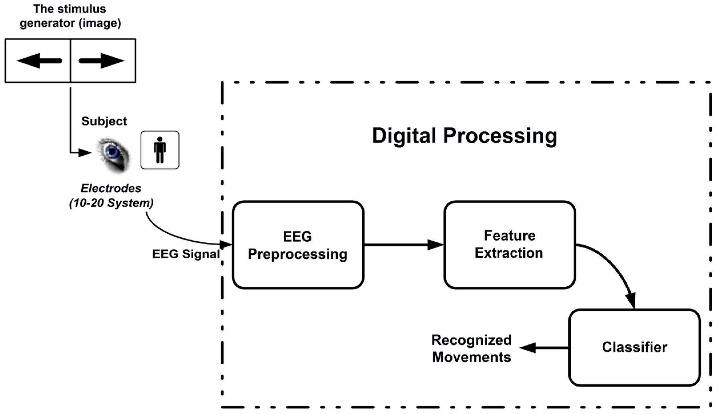
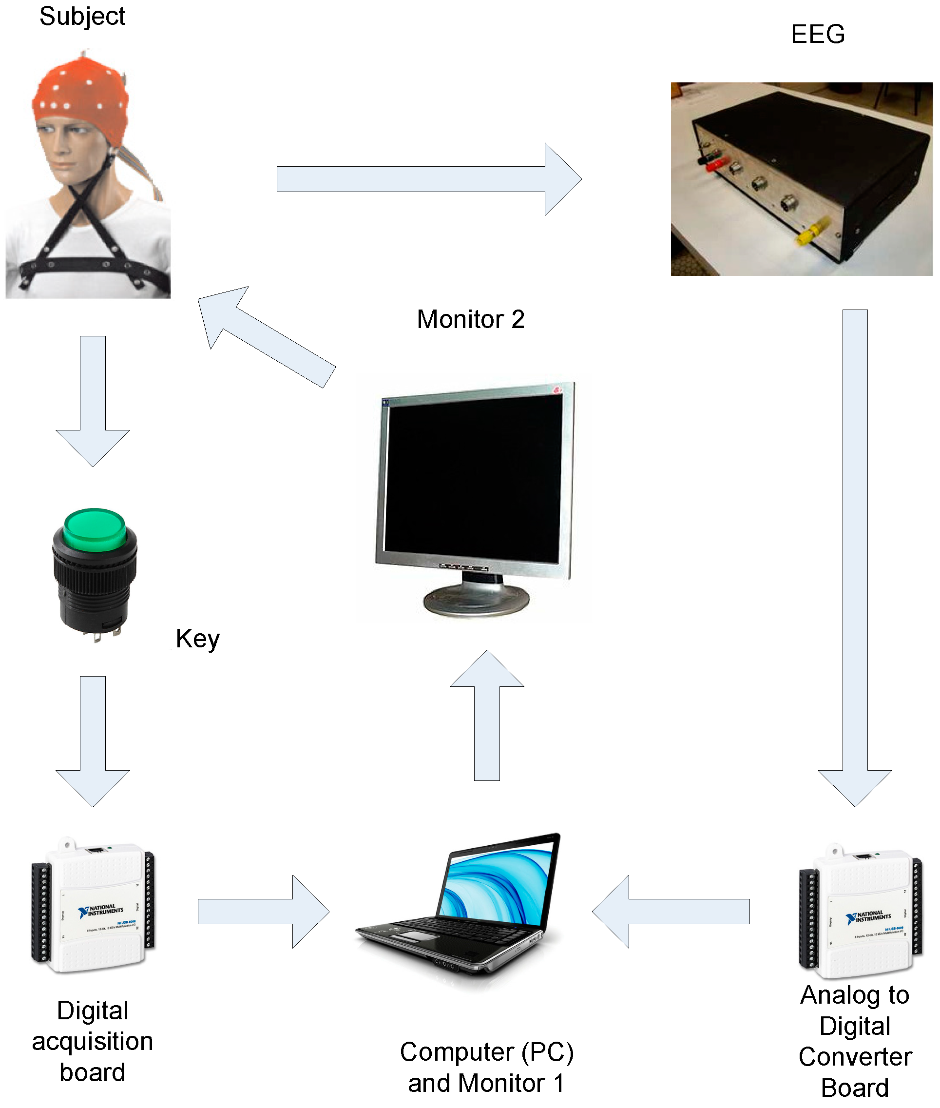
3.1. Materials and Data Synchronization

The proposed experimental BCI system is shown in Figure 2. We have based our experiment on computer-generated stimuli introduced by Monitor 2 to a volunteer who remained sitting in a chair. Data were first obtained from a 10–20 system EEG cap (Spes Medica, CAMSUMA20, Genova, Italy) [40] and then analogically amplified and filtered by an EEG to be digitally converted for the computer through an ADC (Analog to Digital Converter) from National Instruments (NI USB 6008, National Instruments, Austin, TX, USA). A key was placed both on the right and left arms of the chair to be triggered according to the stimulus; the signal reading was held through another ADC (NI USB 6008).

Both stimuli generation and data acquisition were synchronously performed by the computer shown in Figure 2. The acquisition was continuously performed until the ensembles were divided into 8-s windows. Thus, the stimuli presentation was synchronized in time to the signal by software. The stimuli sequence shown in Figure 3 was submitted as the following:

(1)

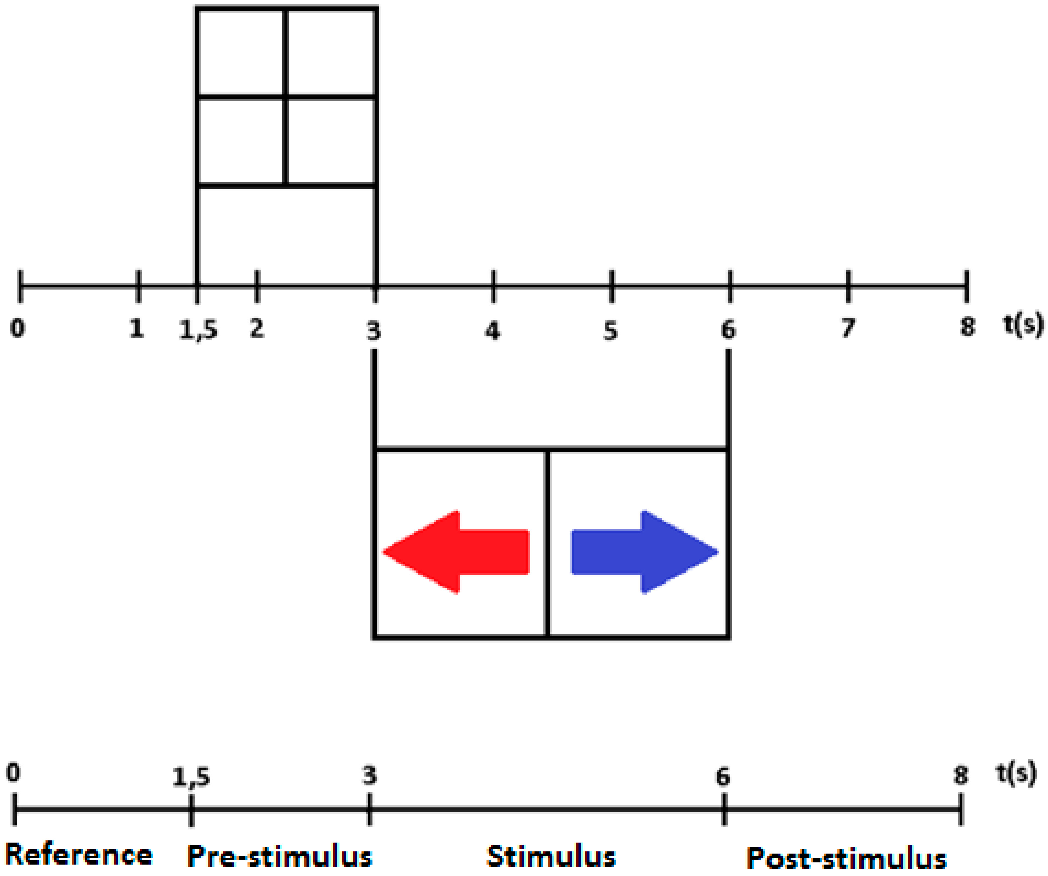
From 0 to 1.5 s: a white screen appeared establishing the so-called reference period;

(2)

From 1.5 to 3 s: a pre-stimulus a cross appeared on the screen;

(3)

From 3 to 6 s: the stimulus presentation occurred (a blue arrow pointing to the right or a red arrow pointing to the left);

(4)

From 6 to 8 s: a white screen appeared once again establishing the so-called post-stimulus period.

This experiment was based on previous studies [22,28] that proved that there exists a large bilateral desynchronization within the frequency bands of both µ and β rhythms during movement imagination, which always keep the energy ipsilateral to the movement superior to the energy contralateral to the movement. Such studies proved that during brief periods (from 1 to 3 s), the movement imagination shows a difference in energy within µ and β rhythms that is capable of distinguishing a movement from another. The choice of using the 8-swindow occurred experimentally.

Along the experiment, the volunteer was asked to push the mechanical keys installed on the chair. Every time a red arrow appeared on the screen, indicating the left-hand movement, the volunteer had to push the key located on the left arm of the chair using his left hand. Whenever a blue arrow appeared, he/she had to perform the same action, but this time using his/her right hand. Such an experiment was held in a synchronous way, i.e., it was possible to control the time when the movement was performed [41], supporting the identification of the ERS/ERD effect during the signal analysis. A post-stimulus period was generated in order to allow the brain enough time to return to its normal state after movement performance [42].

Figure 2. Block diagram of the proposed experiment.

Figure 2. Block diagram of the proposed experiment.

Figure 3. Ensemble time scale.

Figure 3. Ensemble time scale.

The ADC (NI USB6008) was configured to acquire 6 EEG channels (F3, F4, C3, C4, P3 and P4) with a sample frequency of 256 Hz. These channels were selected to cover the most important areas related to the motor cortex. For data configuration, acquisition and synchronization, we developed two software systems through the LabVIEW (Version 2009) development tool. One works like a control software (Software I) and is responsible for calling out the other (Software II), as well as gathering data and managing the digital-analog acquisition (Figure 2). The acquisition must be synchronized with stimuli presentation performed by Software II (Monitor 2), which is responsible for triggering the acquisition process by communicating with Software I (Monitor 1). Next, the presentation of a pre-determined number of ensembles starts as Software I saves the corresponding data; the sequence generating stimuli is randomly created and differs from one experimental run to another. Moreover, Software II also controls and saves data obtained from the keys. For this experiment, key control was performed, so that the volunteer could have a 1-s window after stimulus presentation (from 3 to 4 s) to push the key, so as to guarantee that it did not react if pushed before or after the appearing of the window.

The synchronization between stimulus presentation and time base (where the first sample equals 0 s and the $n$ sample equals $n\times T$ s; $T$ s being the sample period) was tested through feedback in the acquisition board. The acquisition board has analog inputs for A/D conversion, as well as digital inputs and outputs at TTL (Transistor-Transistor Logic) voltage levels. The feedback consisted of linking 2 digital outputs (S₀ and S₁) to 2 analog channels and codifying each segment through digital outputs. A small change was implemented in the Software II, so as to cause the digital output values to change according to a certain established pattern when changing the ensemble segment, e.g., as in the passage from the reference period to pre-stimulus.

The outputs connected to the 2 analog channels remained in their logic states during the whole period of the observed segment. Along the stimulus period, for instance, S₀ remained at a high logic level (5 V), while S₁ remained at a low logic level (0 V) during all 3 s. Therefore, it was possible to verify whether the transitions and the time base of data acquisition occurred synchronously by checking the data obtained through analog channels.

3.2. EEG Signal Processing

EEG signal preprocessing consists of applying a band pass filter both in µ and β rhythms (4th order Butterworth digital filter) and separating signals into ensembles according to each movement class (right or left). The Software I registers both the synchronism data and the pushed button. Data are then separated regarding both the class and the pushed button, e.g., in the case of the synchronism file indicating an ensemble pointing the arrow to the left and the volunteer pushes the right button or no button at all, the segment acquired is then automatically discarded.

CSP Filter

For our purposes, the first step to calculate the spatial filter W is to estimate the co-variance matrices of the training set using Equation (6). It is important to notice that every time the CSP filter was calculated, we used only the training set.

In order to maximize the discriminatory activity between the two classes during hand movement, we applied both 1- and 2-s windows to the EEG signal to further extract the channels’ spectral components and variances that best discriminate the classes in terms of the determined eigenvalues. According to previous studies, the ERD/ERS effects usually occur up to 2 s after movement performance [27,41,42]. Thus, we considered times 3 and 4 s of the ensemble shown in Figure 3 as the starting points of the window. Accordingly, to calculate W we need to:

(1)

Estimate ${\Sigma }^{\mathbf{\text{L}}}$ and ${\Sigma }^{\mathbf{\text{R}}}$ (which are the co-variance matrices for the left and right classes, respectively) through the training set;

(2)

Find the matrix $\Sigma ={\Sigma }^{\mathbf{\text{R}}}+{\Sigma }^{\mathbf{\text{L}}}$;

(3)

Perform the “whitening” operation in order to obtain the matrix P;

(3)

Decompose ${\Sigma }^{\mathbf{\text{L}}}$ and ${\Sigma }^{\mathit{R}}$ through matrix P to obtain the matrices $S^{\mathbf{\text{L}}}$ and $S^{\mathbf{\text{R}}}$, whose eigenvalues ${\Lambda }^{\mathbf{\text{L}}}$ and ${\Lambda }^{\mathbf{\text{R}}}$ represent the discriminatory activity in the new CSP channel space;

(5)

Select both the $n$ largest eigenvalues ${\Lambda }^{\mathbf{\text{L}}}$ and ${\Lambda }^{\mathbf{\text{R}}}$ that will maximize the variance in the left-hand movement condition while minimizing the variance in the right-hand movement condition;

(6)

Calculate the spatial filter and select $2\times n$ columns of the matrix W, which are related to the $n$ largest eigenvalues of ${\Lambda }^{\mathbf{\text{L}}}$ and ${\Lambda }^{\mathbf{\text{R}}}$, respectively.

To successfully accomplish the EEG signal classification, we need to properly choose the features; that is, for the LDA classifier, the energy of the two best CSP channels (for the NB classifier, Welch periodogram’s components are also used) that allow identifying and classifying both right- and left-hand movements. Many authors use algorithms to verify each feature’s relevance [43]. For this experiment, the manual method for choosing features performed by an expert was applied. Using an expert to virtually select the best features is a common practice that many times generates higher hit rates than automatic methods [41,43].

3.3. Features Extraction

It is important to notice that all of the features were selected using only the training set.

3.3.1. Energy of CSP Filtered EEG

The feature extracted through CSP filters is the logarithm of the energy of the signal projected with the best eigenvalues for each class. Accordingly:

$$\mathit{f}\mathit{e}\mathit{a}\mathit{t}\mathit{u}\mathit{r}{\mathit{e}}_j=\log \left({\mathit{w}}_{\mathit{j}}^{\mathit{T}}\times \mathit{X}\times {\mathit{X}}^{\prime }\times {\mathit{w}}_{\mathit{j}}\right)$$

(17)

where $\mathit{f}\mathit{e}\mathit{a}\mathit{t}\mathit{u}\mathit{r}{\mathit{e}}_j$ is the feature vector used for classification and ${\mathit{w}}_{\mathit{j}}$ is the $j$-th spatial filter. Operation $\log ()$ is applied in order to approach energy distributions as close as possible to a Gaussian. The EEG signal segment X is obtained considering previous discussions. The expert chooses the features for the column of the filter $\mathit{W}$ with the highest discriminatory activity.

3.3.2. Welch’s Periodogram Components

The first step to determine the spectral components was to find the initial instant of the cut of the window, by using the training set. It is well known that the ERD/ERS effects can occur during movement and/or movement planning, mainly in µ and β rhythms, where the signal is filtered. After band pass filtering it, the signal was squared to obtain its energy. Next, we calculated the energy average of all ensembles in each class to verify the ERD/ERS evidence, as described by [27,42]. The average energy of each channel is given by:

$$Energy=\frac{1}{M}{\displaystyle \sum }_{i=0}^M{C}_{ji}^{{(c)}^2}$$

(18)

where $C_j^{(c)}$ is the channel $j$ of the EEG signal in condition $(c)$ and M is the number of ensembles. To better visualize the data, a moving average filter was applied to the resulting signal, so as to smooth it. Results show the time instant in which the ERD/ERS occurs, determining the initial instant to be windowed. Effects are expected to be more prominent from the instant of the movement to about 2 s after it. Once the initial instant of the “windowing” was obtained, Equation (3) was applied within a 2-s window. For a 2-s window at 50% overlap, we used three 1-s windows, as shown in Figure 4.

Figure 4. Windowing for a 2-s segment at 50% overlap between windows according to the Welch method.

Figure 4. Windowing for a 2-s segment at 50% overlap between windows according to the Welch method.

By using 1-s windows, it was possible to obtain a frequency resolution of 1 Hz between each spectral component. Values were represented by graphs, as well as the lateralization index (LI), which shows the difference of energy between the right and left hemispheres [27,44]:

$$LI=\left[\left(EnergyLC{H}_{leftmovement}-EnergyRC{H}_{leftmovement}\right)+\left(EnergyRC{H}_{rightmovement}-EnergyLC{H}_{rightmovement}\right)\right]/2$$

(19)

where the Energy LCH of the channels in the left hemisphere and Energy RCH is the energy of channels in the right hemisphere. Energy LI values indicate a high contralaterality of the signal. By applying them to the energy of each frequency component, it was possible to observe which components best discriminate the classes. The LI can also be obtained in the time domain, so as to verify in which instants the highest LI values occur, indicating a larger discriminatory activity. The expert uses the components with high LI to compose the set of features.

Moreover, same spectral components used by [29,45,46,47] to classify EEG signals are suggested as features. In order to reach a good spectral component resolution, a rectangular window was used, since it possesses the lower central lobe. We separated it into three 1-s windows at 50% overlap between each window, as shown in Figure 4. The feature vector is given by:

$$\mathit{f}\mathit{e}\mathit{a}\mathit{t}\mathit{u}\mathit{r}{\mathit{e}}_{\mathit{F} }= \text{log}(\widehat{Gxx}\left(F\right) )$$

(20)

where $\mathit{f}\mathit{e}\mathit{a}\mathit{t}\mathit{u}\mathit{r}{\mathit{e}}_{\mathit{F}}$ is the feature vector used for signal classification and $\widehat{Gxx}\left(F\right)$ is the vector containing the estimated frequency components. Notice that it is not necessary to use all frequency components, but only the best ones. It is important to verify that operation $\log ()$ was applied in order to normalize the distributions. Time T (from the beginning of the “windowing”) was determined according to the considerations mentioned before.

In this study, both NB and LDA classifiers were used. The NB classifier is responsible for modeling the distributions. Since features were normalized through the $\log ()$ function, the normal distribution was used. The features’ vectors and quantity provide the number of distributions. For comparison, the LDA classifier was used in order to determine both the vector ${\mathit{p}}_{\mathit{j}}$ and the constant $p_0$. The number of constants of the vector ${\mathit{p}}_{\mathit{j}}$ is given by the amount of features used. It is important to point out that using large amounts of features in a linear classifier can cause an overfitting [37].

4. Results and Discussion

Our findings came from ten volunteer sin an uncontrolled environment.

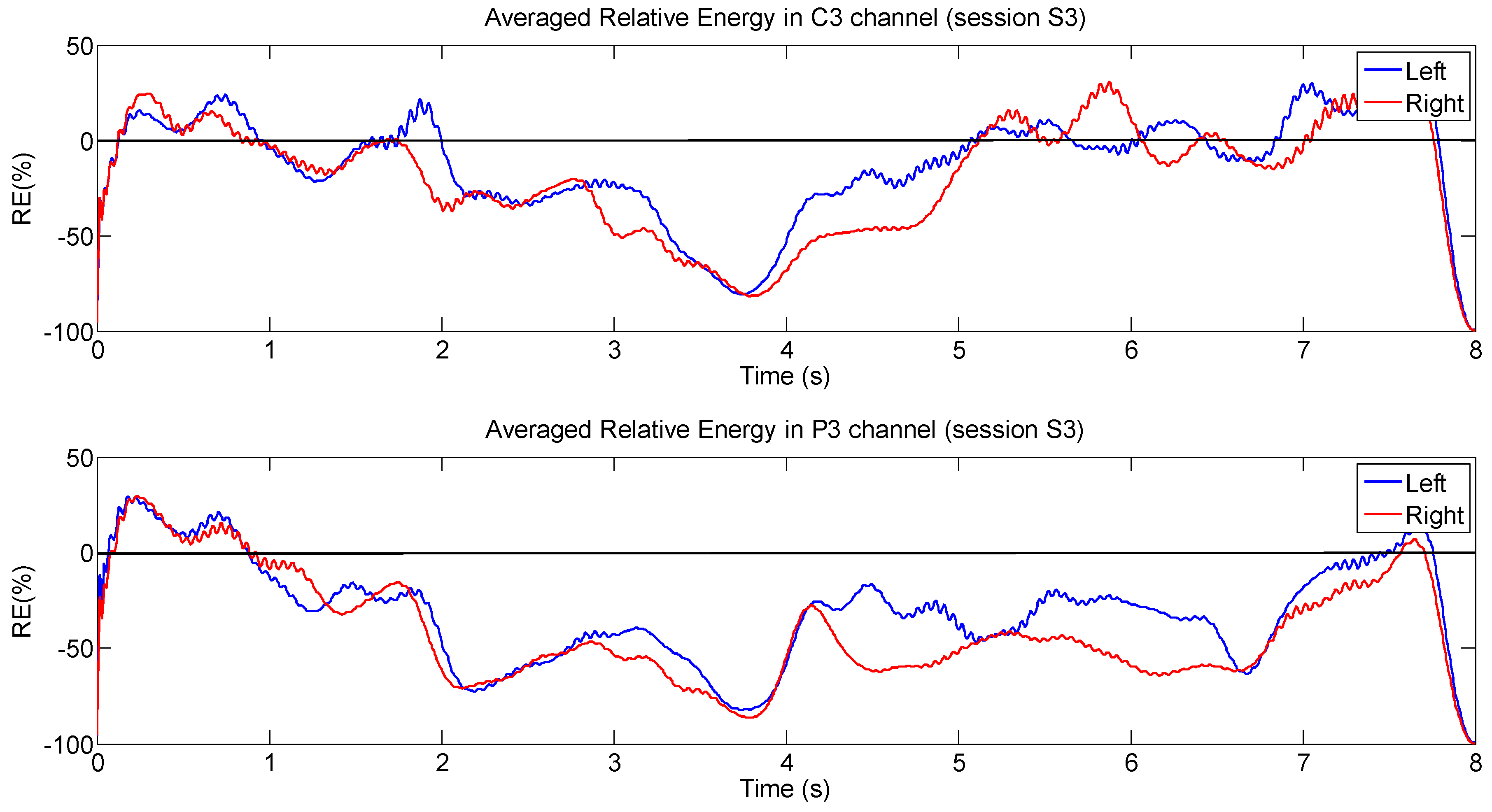
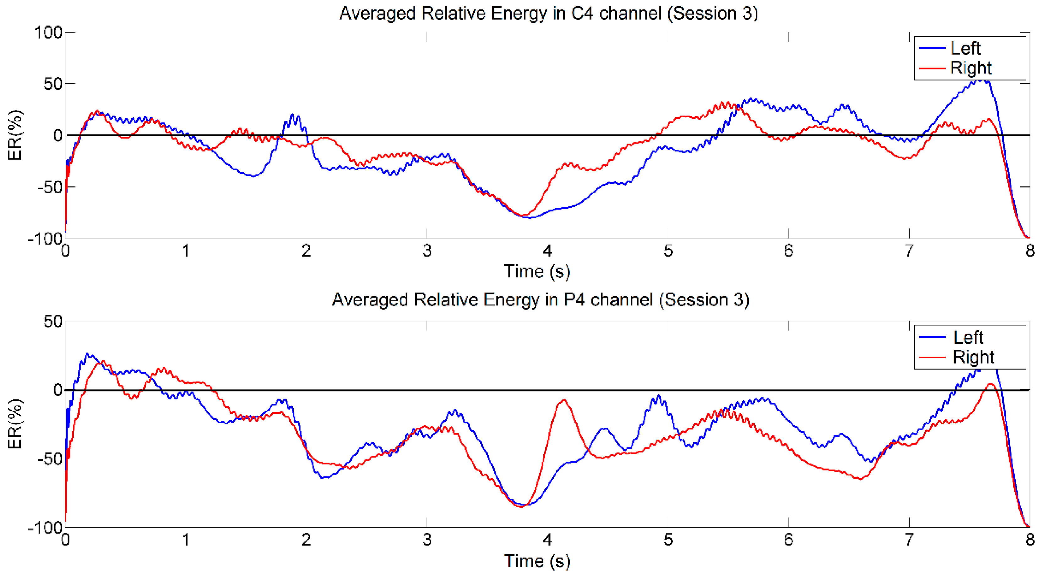
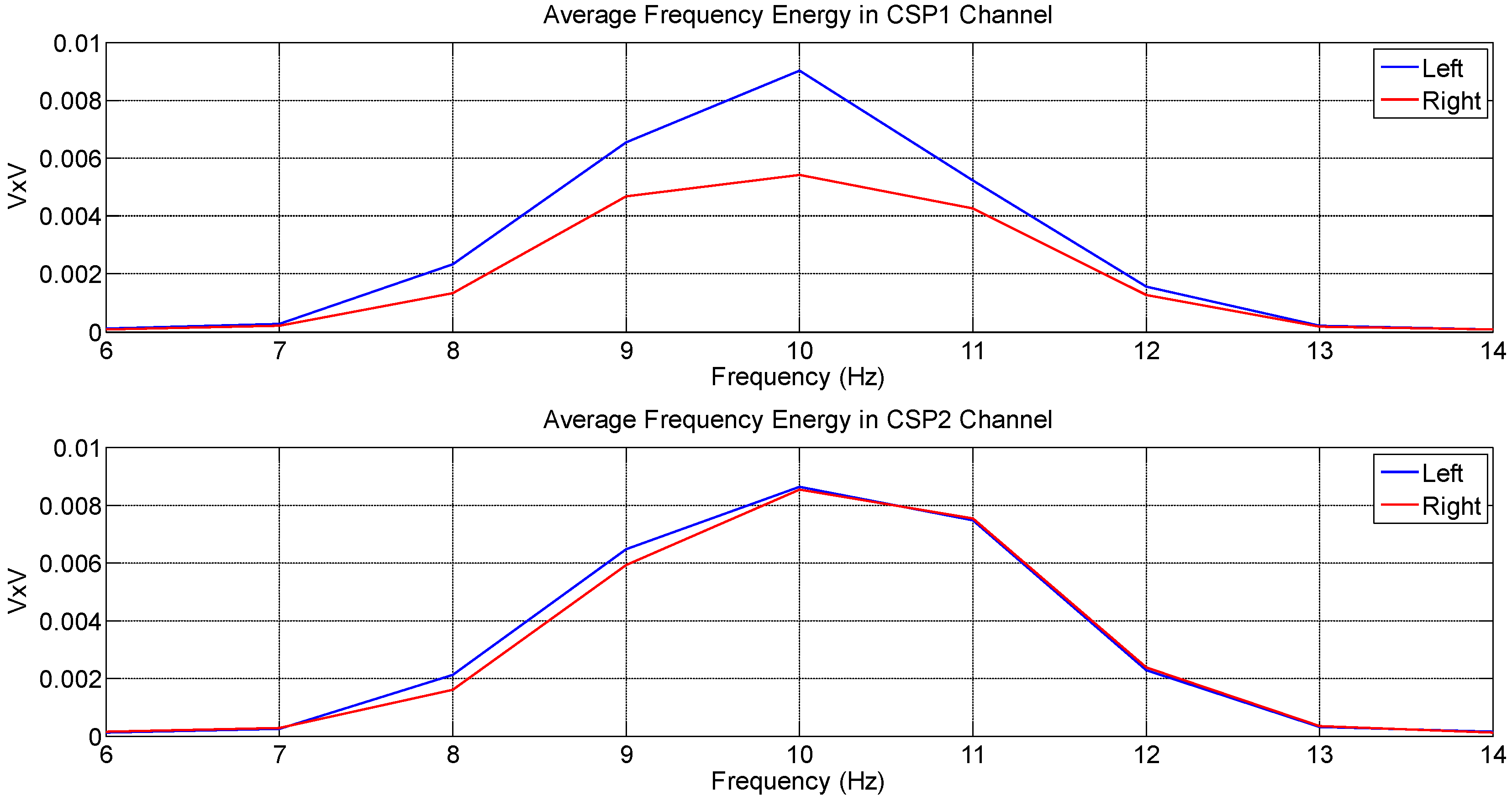
4.1. Analysis Based on Signal Energy

Through the signal energy and the LI analysis over time, it was possible to identify when the ERD/ERS occurred and to determine when the signal should be windowed in order to extract its features, so as to better discriminate movement classes. An analysis of the LI average energy of all of the EEG signal ensembles over time was held. The experiment had four sessions performed (S₁ to S₄) of up to 140 ensembles. However, the amount of ensembles varied according to the movement, since only the ensembles in which the volunteers had pushed the correct button were selected.

As an example, Figure 5 and Figure 6 show a graphic result of the analysis of the relative average energy of the signal for C3 and P3 channels and C4 and P4 channels, respectively, in session S₃. Both channels were band pass filtered in the µ band (from 8 to 12 Hz), and a 63-point moving average filter was applied over the average signal, so as to smooth the graph lines. In the y-axis is shown the relative energy between the reference times, while the x-axis shows time periods. Accordingly, it was possible to visualize how much the energy increases or decreases between no activity at all (reference period) and the performed movement (stimulus).

Figure 5. Relative average energy of channels C3 and P3 during S₃ (μ rhythm).

Figure 5. Relative average energy of channels C3 and P3 during S₃ (μ rhythm).

Figure 6. Relative average energy of channels C4 and P4 during S₃ (μ rhythm).

Figure 6. Relative average energy of channels C4 and P4 during S₃ (μ rhythm).

Results show a strong desynchronization about 500 ms after pre-stimulus presentation at 1.5 s in channels C3 and P3 for both types of movement (Figure 5). ERD/ERS effects can be observed both during and after movement in the channel covering the motor cortex (C3), always keeping the energy ipsilateral to the movement superior to the energy contralateral to the movement; however, an ERS appeared to be sharpest in the left hemisphere. The same effect had been observed in channels covering the parietal lobe, indicating motor activity. Notice that in all cases, the ERS effect of the ipsilateral side occurred about 800 ms after the arrow pointed at time 3 s, indicating a discriminatory effect between the energy of both classes. Thus, in order to extract the spectral components and the signal energy for signal windowing, we used initial values between 3.5 and 4 s (from 500 ms to 1 s after the appearance of the arrow). No discriminatory activity was observed in β rhythm and channels F3 and F4. Therefore, no signal from β rhythm was used for classification process, since it showed no relevant discriminatory feature.

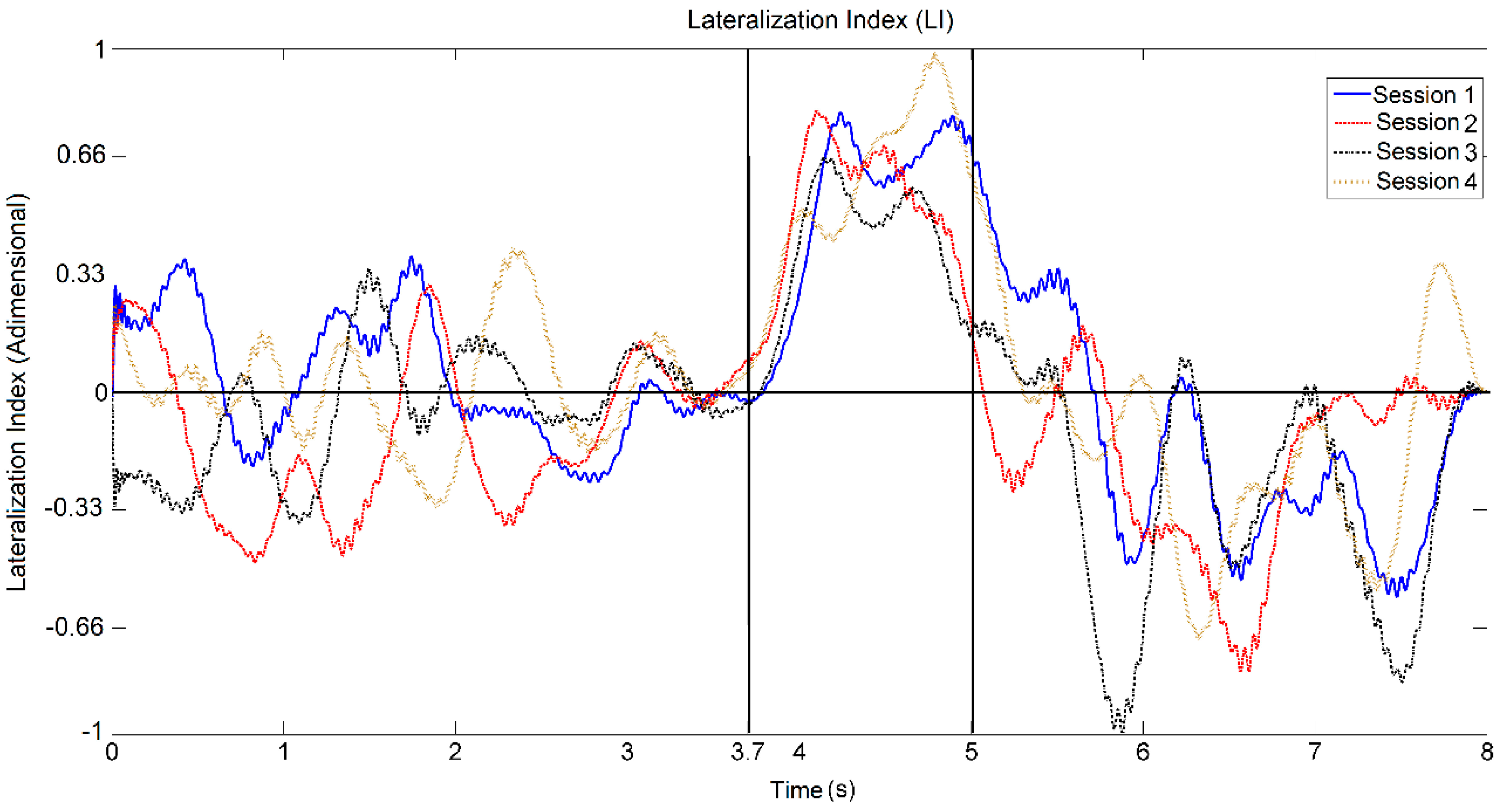
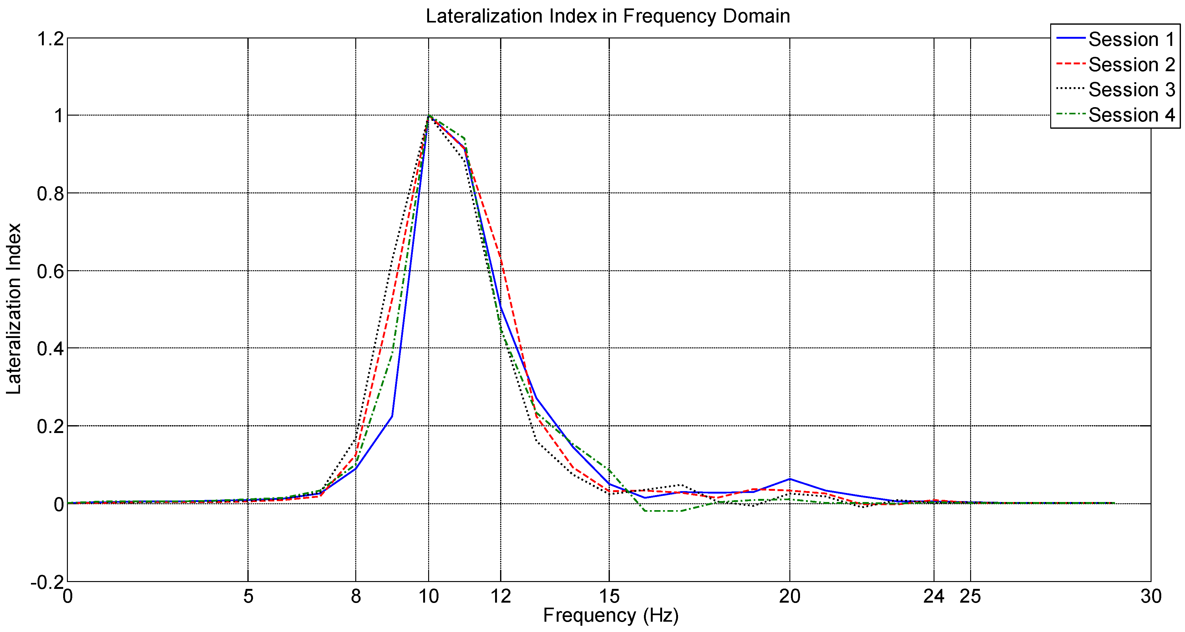
4.2. Analysis Based on LI

The LI was calculated through central channels (C3 and C4) and parietal channels (P3 and P4) only, using Equation (20), since they showed motor activity. Figure 7 shows the normalized LI average graph over time for all four sessions. LI results indicate a high signal lateralization on the central lobe from about 500 ms after the appearing of the arrow to about 2 s after its appearing at 5 s, corroborating the choice of starting the windowing at 3.5 s. The graph is normalized, and also note that when the curves are above the zero line, this indicates that an ERD is occurring; when below zero, this indicates that an ERD is occurring, and when is below zero, this indicates that an ERS is occurring, according to Equation (20).

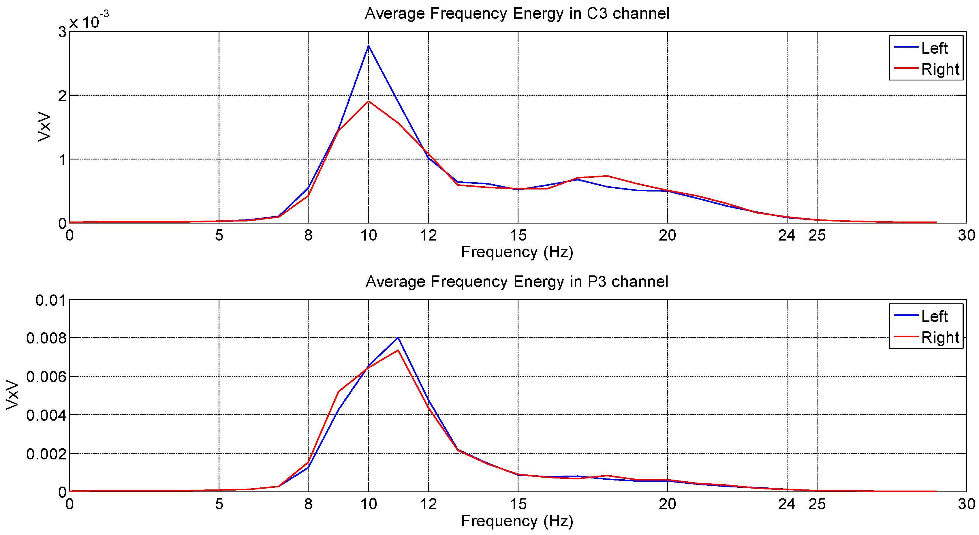
4.3. Analysis Based on the Welch Periodogram

This session shows the results obtained from the periodogram. The LI (see Figure 8) of the spectral components was also evaluated to determine which frequency components presented a larger discrimination. A 2-s window was used to obtain a frequency resolution of at least 1 Hz; signals were filtered by a band pass between 8 and 24 Hz, so as to entirely cover the sensorimotor rhythm. Only as an example, Figure 9 shows the analysis in the frequency of the experiment in session S₃. Our findings show a clear energy distinction between the movement classes in µ rhythm on channel C3 and a slightly distinction on channel P3, always keeping the energy ipsilateral to the movement superior to the energy contralateral to the movement. We found similar results for channels C4 and P4. No relevant discriminatory activity was observed within β rhythm, since, as mentioned before, there is no perceptive discriminatory activity in β rhythm regarding the volunteers.

Figure 7. Relative average LI for channels C3, C4, P3 and P4 in all sessions.

Figure 7. Relative average LI for channels C3, C4, P3 and P4 in all sessions.

Figure 8. LI on the frequency domain for all sessions.

Figure 8. LI on the frequency domain for all sessions.

Figure 9. Average energy on the frequency domain for channels C3 and P3.

Figure 9. Average energy on the frequency domain for channels C3 and P3.

4.4. Analysis Based on the Spatial Filter

In order to analyze the CSP filter, its coefficients had to be calculated based on the entire database and then applied to it. Filters were calculated through a two-second window starting at 3 s. These windows were chosen, because an evaluation of the filter functionality showed whether the segment of the signal creates a new channel space with discriminatory activities by analyzing the selected segment. As mentioned before, only central and parietal channels were considered for calculating the coefficients of the filter. Signals were filtered within µ rhythm. Original channels (C3, C4, P3 and P4) were linearly combined by the filter W obtained according to our methodology, so as to create a new space of channels, which were named CSP1, CSP2, CSP3 and CSP4. As an example, Figure 10 shows the average energy in the frequency domain for channels CSP1 and CSP2.

Figure 10. Average energy in the frequency domain for channels CSP1 and CSP2. CPS, common spatial pattern.

Figure 10. Average energy in the frequency domain for channels CSP1 and CSP2. CPS, common spatial pattern.

The eigenvalues matrices ${\Lambda }^{(\mathbf{\text{R}})}$ and ${\Lambda }^{(\mathbf{\text{L}})}$ indicate which channels present the highest discriminatory activity. Notice that the results obtained from ${\Lambda }^{(\mathbf{\text{R}})}$ and ${\Lambda }^{(\mathbf{\text{L}})}$ are in agreement with the graphic results. In channel CSP1 (${\Lambda }^{(k)}$ first column), ${\Lambda }^{(\mathbf{\text{R}})}$ has minimum value and ${\Lambda }^{(\mathbf{\text{L}})}$ has maximum value, indicating that the left movement class energy should be superior to the right movement class energy (also, ${\Lambda }^{(\mathbf{\text{R}})}+ {\Lambda }^{(\mathbf{\text{L}})}=I$):

$${\Lambda }^{(\mathbf{\text{R}})}=\begin{array}{cccc}0.37& 0& 0& 0\\ 0& 0.47& 0& 0\\ 0& 0& 0.50& 0\\ 0& 0& 0& 0.54\end{array}$$

(21)

The first and only column of matrices ${\Lambda }^{(\mathbf{\text{R}})}$ and ${\Lambda }^{(\mathbf{\text{L}})}$ shows the filters that best discriminate both classes, which is also in agreement with our graphic results. Applying the filter had also increased the discriminatory activity between both movement classes. We could verify this by analyzing the proportional energy between both classes for the same channel, according to:

$$E_P^{(c)}=\frac{E^{(c)}}{E^{(R)}+E^{(L)}}$$

(22)

where $E_P^{(c)}$ is the proportional energy in class $(c)$, $E^{(c)}$ is the energy of class (c) and $E^{(R)}$ and $E^{(L)}$ are the energies of the right class movement and the left class movement, respectively. By verifying the proportional energy in the right class for the 10-Hz component for the channel C4 of the original sensor space, for instance, we obtained the results shown in Table 1.

Thus, filter application increased the contrast between both classes according to the results. It is important to point out that the coefficients were estimated from all databases; for classification, however, the training set only was used.

Table 1. A comparison of the proportional energy between classes with and without the CSP filter.

Without CSP Filter, Channel C4	With CSP Filter, Channel CSP4
${\mathit{E}}_{\mathit{P}}^{(\mathit{R})}$ = 0.59	${\mathit{E}}_{\mathit{P}}^{(\mathit{R})}$ = 0.63

Table 1. A comparison of the proportional energy between classes with and without the CSP filter.

Without CSP Filter, Channel C4	With CSP Filter, Channel CSP4
${\mathit{E}}_{\mathit{P}}^{(\mathit{R})}$ = 0.59	${\mathit{E}}_{\mathit{P}}^{(\mathit{R})}$ = 0.63

4.5. Classification Based on Signal Energy

Results shown in this session were obtained from the cross-correlation procedure, where 9/10 of the data were separated for training and 1/10 for classification. The training and classification procedure were performed 100 times; both training and testing data were selected randomly. The classification rate was given by the average of all performances. The standard deviation is also presented.

The spatial filter was calculated first through four channels (C3, C4, P3 and P4) and then through two channels (C3 and C4). Calculating the filter through four channels allowed a new channel space with four CSP channels, where the two columns of filter W with the highest eigenvalues of each class were tested. All resulting channels (CSP channels) were considered. Calculating the filter through two channels allowed two new CSP channels to be used to calculate the classifier. As an example, Table 2 shows all four resulting CSP filters. Following the same methodology, Table 3 shows the results obtained from the NB classifier.

Table 2. Average hit rates with the LDA classifier using CSP channels and channels C3, C4, P3 and P4 to estimate W.

Window	Hit rate by session (% average ± standard deviation)
	S1	S2	S3	S4
W1	66.8 ± 10.6	68.5 ± 8.72	69.0 ± 10.3	64.8 ± 9.48
W2	66.5 ± 10.7	67.0 ± 8.91	69.9 ± 10.6	64.5 ± 7.95
W3	65.2 ± 9.51	66.8 ± 8.88	70.6 ± 10.1	65.1 ± 7.62
W4	66.7 ± 9.13	66.4 ± 8.45	68.5 ± 9.91	66.8 ± 8.77
W5	64.1 ± 10.6	67.8 ± 8.24	69.6 ± 9.01	65.4 ± 8.71
W6	64.9 ± 9.73	66.4 ± 8.71	68.1 ± 11.2	67.4 ± 9.12

Table 2. Average hit rates with the LDA classifier using CSP channels and channels C3, C4, P3 and P4 to estimate W.

Window	Hit rate by session (% average ± standard deviation)
	S1	S2	S3	S4
W1	66.8 ± 10.6	68.5 ± 8.72	69.0 ± 10.3	64.8 ± 9.48
W2	66.5 ± 10.7	67.0 ± 8.91	69.9 ± 10.6	64.5 ± 7.95
W3	65.2 ± 9.51	66.8 ± 8.88	70.6 ± 10.1	65.1 ± 7.62
W4	66.7 ± 9.13	66.4 ± 8.45	68.5 ± 9.91	66.8 ± 8.77
W5	64.1 ± 10.6	67.8 ± 8.24	69.6 ± 9.01	65.4 ± 8.71
W6	64.9 ± 9.73	66.4 ± 8.71	68.1 ± 11.2	67.4 ± 9.12

Table 3. Average hit rates with the NB classifier using all CSP channels and channels C3, C4, P3 and P4 to estimate W.

Window	Hit rate by session (% average ± standard deviation)
	S1	S2	S3	S4
W1	66.1 ± 10.5	66.2 ± 9.32	64.3 ± 9.76	62.9 ± 9.34
W2	64.4 ± 10.7	64.6 ± 8.86	64.6 ± 10.6	62.4 ± 8.15
W3	63.6 ± 9.93	65.2 ± 8.40	65.2 ± 10.6	62.1 ± 8.55
W4	64.6 ± 11.4	63.5 ± 8.50	65.0 ± 9.87	62.0 ± 9.85
W5	62.6 ± 10.5	65.1 ± 8.87	65.0 ± 10.4	59.7 ± 9.32
W6	63.1 ± 10.1	64.0 ± 8.94	62.6 ± 9.55	59.5 ± 9.34

Table 3. Average hit rates with the NB classifier using all CSP channels and channels C3, C4, P3 and P4 to estimate W.

Window	Hit rate by session (% average ± standard deviation)
	S1	S2	S3	S4
W1	66.1 ± 10.5	66.2 ± 9.32	64.3 ± 9.76	62.9 ± 9.34
W2	64.4 ± 10.7	64.6 ± 8.86	64.6 ± 10.6	62.4 ± 8.15
W3	63.6 ± 9.93	65.2 ± 8.40	65.2 ± 10.6	62.1 ± 8.55
W4	64.6 ± 11.4	63.5 ± 8.50	65.0 ± 9.87	62.0 ± 9.85
W5	62.6 ± 10.5	65.1 ± 8.87	65.0 ± 10.4	59.7 ± 9.32
W6	63.1 ± 10.1	64.0 ± 8.94	62.6 ± 9.55	59.5 ± 9.34

In general, no relevant variance on classification rates for differently-sized windows was observed. However, we noticed a large variability among sessions; S₃ indicated the highest hit rate. It is not possible to confirm whether the window size influenced it due to the high standard deviation found in the results; the variances among the types of window are smaller than the standard deviation of each window in the same session. Using two channels (C3 and C4) to estimate the spatial filter coefficients together with the two resulting CSP channels allowed for classification rates closer to that of using four channels (C3, C4, P3 and P4) to estimate the filter coefficients through the four resulting CSP channels. The worst result came from the tow CSP channels obtained by calculating the coefficients through all four EEG signals. These findings provide a good indication that using small windows (about 1 s) is an advantage, since it reduces the processing time, a common concern for systems tested online.

We also noticed that the increase of channels degraded the classification rates mainly for sessions S₃ and S₄. Its probable cause is the fact that only two channels (C3 and C4) showed high motor activity. Studies reporting the occurrence of high hit rates following this same methodology usually have a larger amount of channels, using 55 and 56 channels of a modified 10–20 system. Larger amounts of channels increase the resolution in the motor area, providing more discriminatory information among classes than only four channels, which probably leads to better classification rates. High variability indexes caused by high leakages indicate that classification depends both on training and testing sets, which is a common characteristic in this kind of study [36]. As a comparison, Table 4 shows the hit rate obtained only from channels C3 and C4 in session S3. Results were found by substituting matrix W with the identity matrix. Using an unfiltered signal allowed slightly lower rates than using a filter calculated by two EEG and two CSP channels and estimated by four EEG channels considering four CSP channels as the input characteristic. However, it is not possible to verify whether using the filter had significantly improved the classification result, because of the high variability. In order to verify whether the filter increases the EEG signal hit rate, further studies using larger amounts of channels covering the motor area and removing artifacts are necessary.

The LDA classifier again showed classification rates higher than the NB classifier. Using smaller windows significantly degraded classification, indicating that a significant amount of data is necessary for energy estimation. It is worth mentioning that the expected value of the signal energy gets closer to the real value by increasing the number of samples for its estimation [30]. Thus, smaller windows have a higher variability of values, which degrades the classification rate. Using higher sampling rates can lead to a better characterization of the signal energy in smaller windows.

Table 4. Average hit rates using channels C3 and C4 for classification.

Window	Hit rate session S3 (% average ± standard deviation)
	LDA	Naive Bayes
W1	67.8 ± 9.75	63.2 ± 10.5
W2	68.3 ± 8.85	63.3 ± 10.0
W3	68.2 ± 10.4	63.7 ± 11.5
W4	67.1 ± 9.65	63.3 ± 8.68
W5	68.8 ± 10.2	63.1 ± 10.7
W6	66.7 ± 9.65	61.2 ± 10.1

Table 4. Average hit rates using channels C3 and C4 for classification.

Window	Hit rate session S3 (% average ± standard deviation)
	LDA	Naive Bayes
W1	67.8 ± 9.75	63.2 ± 10.5
W2	68.3 ± 8.85	63.3 ± 10.0
W3	68.2 ± 10.4	63.7 ± 11.5
W4	67.1 ± 9.65	63.3 ± 8.68
W5	68.8 ± 10.2	63.1 ± 10.7
W6	66.7 ± 9.65	61.2 ± 10.1

4.6. Classification Based on the Spectral Components as the Input Feature

This session shows the classification results obtained from spectral components. The components selected according to the higher values given by the LI index of the frequencies were inserted into the features vector. As a comparison, we used 2, 4 and 10 spectral components with two (C3 and C4) and four (C3, C4, P3 and P4) channels. It is worth mentioning that the amount of features is given by the product of the number of spectral components by the number of channels. Table 5 and Table 6 show the results of four sessions using two and four channels, respectively.

Table 5. Average hit rates using the spectral components of two channels (C3 and C4).

Session	Spectral Components
	2		4		10
	LDA	NB	LDA	NB	LDA	NB
S1	62.5 ± 16.6	62.9 ± 17.5	62.5 ± 13.3	65.4 ± 15.3	61.2 ± 16.6	63.5 ± 16.3
S2	60.7 ± 14.9	52.8 ± 12.4	61.6 ± 13.6	55.7 ± 13.9	61.9 ± 14.5	56.1 ± 14.5
S3	60.9 ± 16.0	57.3 ± 15.9	60.6 ± 15.2	56.8 ± 15.2	60.6 ± 13.5	60.3 ± 14.3
S4	62.4 ± 14.0	59.4 ± 13.1	60.9 ± 11.8	58.8 ± 11.9	68.4 ± 11.8	65.4 ± 11.6

Table 5. Average hit rates using the spectral components of two channels (C3 and C4).

Session	Spectral Components
	2		4		10
	LDA	NB	LDA	NB	LDA	NB
S1	62.5 ± 16.6	62.9 ± 17.5	62.5 ± 13.3	65.4 ± 15.3	61.2 ± 16.6	63.5 ± 16.3
S2	60.7 ± 14.9	52.8 ± 12.4	61.6 ± 13.6	55.7 ± 13.9	61.9 ± 14.5	56.1 ± 14.5
S3	60.9 ± 16.0	57.3 ± 15.9	60.6 ± 15.2	56.8 ± 15.2	60.6 ± 13.5	60.3 ± 14.3
S4	62.4 ± 14.0	59.4 ± 13.1	60.9 ± 11.8	58.8 ± 11.9	68.4 ± 11.8	65.4 ± 11.6

Table 6. Average hit rates using the spectral components of four channels (C3, C4, P3 and P4).

Session	Spectral Components
	2		4		10
	LDA	NB	LDA	NB	LDA	NB
S1	62.6 ± 16.2	64.9 ± 18.4	59.6 ± 16.1	68.4 ± 17.3	54.6 ± 17.2	65.8 ± 13.5
S2	62.6 ± 13.9	50.7 ± 13.4	64.3 ± 12.5	54.1 ± 14.9	59.3 ± 13.6	51.7 ± 14.8
S3	56.1 ± 15.2	55.7 ± 13.3	52.7 ± 15.9	53.8 ± 16.1	45.9 ± 15.6	51.1 ± 15.9
S4	58.9 ± 12.4	51.0 ± 14.1	60.1 ± 12.6	55.4 ± 13.0	60.8 ± 12.7	54.7 ± 11.9

Table 6. Average hit rates using the spectral components of four channels (C3, C4, P3 and P4).

Session	Spectral Components
	2		4		10
	LDA	NB	LDA	NB	LDA	NB
S1	62.6 ± 16.2	64.9 ± 18.4	59.6 ± 16.1	68.4 ± 17.3	54.6 ± 17.2	65.8 ± 13.5
S2	62.6 ± 13.9	50.7 ± 13.4	64.3 ± 12.5	54.1 ± 14.9	59.3 ± 13.6	51.7 ± 14.8
S3	56.1 ± 15.2	55.7 ± 13.3	52.7 ± 15.9	53.8 ± 16.1	45.9 ± 15.6	51.1 ± 15.9
S4	58.9 ± 12.4	51.0 ± 14.1	60.1 ± 12.6	55.4 ± 13.0	60.8 ± 12.7	54.7 ± 11.9

Our findings indicate a lower average hit rate than those obtained through the energy of the CSP filtered signal. A higher variability was also observed, indicating irregularity in classification rates. The LDA classifier maintained a higher hit rate among sessions, except for S₁ when using four EEG channels. The number of channels had influenced mainly the hit rates given by the NB classifier, probably because the high dependence maintained by the channels’ signals violate its principle of considering only independent features. The number of spectral components had not significantly influenced classification rates, which is an interesting finding, since the number of features directly influences the computational efficiency in online applications. The high variability of the data shows that using this kind of feature made the classifier very dependent on the training set, so as not to generalize data classification in a satisfactory manner.

Results indicate both variability and hit rates similar to those obtained through the signal energy and the CSP filter. These results indicate that using spectral components as input feature requires “well behaved” stationary signals, since it is usually necessary to use larger windows for a good frequency spectrum resolution, so that non-stationary behavior is not desirable. By comparing the laterality indexes over time, we can verify that the volunteers are able to maintain the movement laterality for approximately 1 s between 4 and 5 s. The problem of using much smaller windows is that the loss of frequency leads to the loss of information within the sensorimotor rhythm, since it already has activity in narrow frequency rhythms.

To confirm the investigation, ANOVA and multiple comparisons were used. For the statistical validation methodology, three-factor experiments were used (three-factor fixed effects model). In general, factorial designs are most efficient for this type of experiment. By factorial design, we mean the investigation of all possible combinations of the levels of the factors in each complete trial or replicate of the experiment. ANOVA provides a statistical test of whether or not the means of several groups are all equal. If they are not all the same, you may need information about which pairs of means are significantly different and which are not. A multiple comparison procedure is a test that can provide such information. Two means are significantly different if their intervals are disjoint and not significantly different if their intervals overlap. This experimental design is a completely randomized design. Consider the three-factor factorial experiment with underlying model Equation (23):

$$Y_{ijkl}=\text{μ}+{\text{τ}}_i+{\text{β}}_j+{\text{γ}}_k+{\left(\text{τβ}\right)}_{ij}+{\left(\text{τγ}\right)}_{ik}+{\left(\text{βγ}\right)}_{jk}+{\left(\text{τβγ}\right)}_{ijk}+{ϵ}_{ijkl}\{\begin{array}{c}i=1,2,\dots ,a\\ j=1,2,\dots ,b\\ \begin{array}{c}k=1,2,\dots ,c\\ l=1,2,\dots ,n\end{array}\end{array}$$

(23)

where μ is the overall mean effect, ${\text{τ}}_i$ is the effect of the i-th level of factor A (electrode placement), ${\text{β}}_j$ is the effect of the j-th level of factor B (volunteers), ${\text{γ}}_k$ is the effect of the k-th level of factor C (different sessions), ${\left(\text{τβ}\right)}_{ij}$ is the effect of the interaction between A and B, ${\left(\text{τγ}\right)}_{ik}$ is the effect of the interaction between A and C, ${\left(\text{βγ}\right)}_{jk}$ is the effect of the interaction between B and C, ${\left(\text{τβγ}\right)}_{ijk}$ is the effect of the interaction between A, B and C and ${ϵ}_{ijkl}$ is a random error component having a normal distribution with mean zero and variance σ.

An analysis for an experiment using single factor (classifiers), using analysis of variance, was also made. It was found that the iteration between the classifiers is significant, i.e., they present distinct values for the database presented.

Notice that the model contains three main effects (A, B and C), three two-factor interactions, a three-factor interaction and an error term. The F-test on the main effects and interactions follows directly from the expected mean squares. These ratios follow F distributions under the respective null hypotheses. We used α = 0.05 (significance level). The analysis of variance for a three-factor experiment showed that the main effects, due to the electrode placement, volunteers and different sessions, are significant, i.e., there is strong evidence to conclude that the variances of the three main effects are different.

5. Conclusions

Our findings allow us to conclude that it is possible to classify EEG signals through information about hand movement behavior. We also verified the physiological effect of hand movement in the brain through noninvasive measurements by using six EEG channels. The volunteers showed activity lateral to the movement within the µ rhythm for channels located both in central and parietal areas of the lobe. Activity for central and parietal channels within the β rhythm was also observed; however, no relevant discriminatory activity within this band was verified. The spatial filter did not significantly increase the hit rate in either classifier. This probably happened because the obtained signals did not show good spatial resolution. Besides, there were only six channels available, of which only four showed activities related to sensorimotor rhythms. Furthermore, this technique is highly sensitive to artifacts for filter estimation, and the signals were not handled so as to remove these artifacts. Table 7 presents the classification hit rate for right and left hand of other studies. Note that this studies uses other databases and different feature extraction:

Table 7. Hit rate for other studies.

Classification Method	Accuracy (%)	Reference
Gaussian Support Vector Machines	86	[48]
LDA	61
Multi-Layer Neural Network	80.4	[49]
LDA	80.6
Hidden Markov Model	81.4	[50]
Finite Impulse Neural Network	87.4	[51]
Morlet Wavelet and Bayes Quadratic integrated over time	89.3	[52]
LDA	65.6	[53]

Table 7. Hit rate for other studies.

Classification Method	Accuracy (%)	Reference
Gaussian Support Vector Machines	86	[48]
LDA	61
Multi-Layer Neural Network	80.4	[49]
LDA	80.6
Hidden Markov Model	81.4	[50]
Finite Impulse Neural Network	87.4	[51]
Morlet Wavelet and Bayes Quadratic integrated over time	89.3	[52]
LDA	65.6	[53]

Further studies using a cap with higher electrode resolution are required to validate the CSP filter theory. By using signal energy, with or without the CSP filter, we were able to obtain a good behavior in the classifiers and to maintain the hit rates, even with small one-second windows. The use of spectral components proved to be very sensitive to the quality of the signal and, therefore, a secondary choice for using classification features. In turn, the periodogram proved to be a useful tool to show which frequency bands are more relevant for classification. Using the data obtained through the periodogram together with other preprocessing techniques, such as principal components analysis, allows the development of algorithms for the automatic selection of features. We found lower rates primarily due to the lack of training by the volunteers and feedback, as well as the use of uncertified equipment and experimental runs in an uncontrolled environment. In order to increase the discriminatory activity between the two movement classes, results show the necessity of using feedback during the experiment, such as was performed by the BCI Competition II [28]. Although the LDA classifier had maintained higher rates than the NB classifier, they showed similar performance.

It was possible to confirm whether the use of the LDA is different than NB by the ANOVA analysis, indicating that the use of LDA can improve the classification hit rate rather than NB. Thus, it is possible to say that the statistical parameters of the volunteers are quite distinct from each other. The results of this model showed that the interactions are true once ${\left(\text{τβ}\right)}_{ij}$, ${\left(\text{τγ}\right)}_{ik}$, ${\left(\text{βγ}\right)}_{jk}$ and ${\left(\text{τβγ}\right)}_{ijk}$ are significant.

References

1. Wolpaw, J.R.; Birbaumer, C.; McFarland, D.J.; Pfurtscheller, G.; Vaughan, T.M. Brain-computer interfaces for communication and control. Clinic. Neurophysiol. 2002, 113, 767–791. [Google Scholar] [CrossRef]
2. Neuper, C.; Muller, G.R.; Kubler, A.; Birbaumer, N.; Pfurtscheller, G. Clinical application of an EEG-based brain-computer interface: A case study in a patient with severe motor impairment. Clinic. Neurophysiol. 2003, 114, 399–409. [Google Scholar] [CrossRef]
3. Blankertz, B.; Dornhege, G.; Krauledat, M.; Muller, K.R.; Curio, G. The non-invasive Berlin brain-computer interface: Fast acquisition of effective performance in untrained subjects. NeuroImage 2007, 37, 539–550. [Google Scholar] [CrossRef] [PubMed]
4. Chatterjee, A.; Aggarwal, V.; Ramos, A.; Acharya, S.; Thakor, N.V. A brain-computer interface with vibrotactile biofeedback for haptic information. J. Neuroeng. Rehabil. 2007, 4, 4–40. [Google Scholar] [CrossRef] [PubMed]
5. Kamousi, B.; Amini, A.N.; He, B. Classification of motor imagery by means of cortical current density estimation and Von Neumann entropy for brain-computer interface applications. J. Neural Eng. 2007, 4, 17–25. [Google Scholar] [CrossRef] [PubMed]
6. Pfurtscheller, G.; Brunner, C.; Schlogl, A.; Lopes da Silva, F.H. Mu rhythm (de)synchronization and EEG single-trial classification of different motor imagery tasks. Neuroimage 2006, 31, 153–159. [Google Scholar] [CrossRef] [PubMed]
7. Pineda, J.A.; Silverman, D.S.; Vankov, A.; Hestenes, J. Learning to control brain rhythms: Making a brain-computer interface possible. IEEE Trans. Neural Syst. Rehabil. Eng. 2003, 11, 181–184. [Google Scholar] [CrossRef] [PubMed]
8. Birbaumer, N.; Ghanayim, N.; Hinterberger, T.; Iversen, I.; Kotchoubey, B.; Kubler, A. A spelling device for the paralysed. Nature 1999, 398, 297–298. [Google Scholar] [CrossRef] [PubMed]
9. Bayliss, J.D. Use of the evoked potential P3 component for control in a virtual apartment. IEEE Trans. Neural Syst. Rehabil. Eng. 2003, 11, 113–116. [Google Scholar] [CrossRef] [PubMed]
10. Hoffmann, U.; Vesin, J.M.; Ebrahimi, T.; Diserens, K. An efficient P300-based brain-computer interface for disabled subjects. J. Neurosci. Methods 2008, 167, 115–125. [Google Scholar] [CrossRef] [PubMed]
11. Lalor, E.C.; Kelly, S.P.; Finucane, C.; Burke, R.; Reilly, R.B. Steady-state VEP-based brain-computer interface control in an immersive 3D gaming environment. EURASIP J. Appl. Signal Process. 2005, 2005, 3156–3164. [Google Scholar] [CrossRef]
12. Middendorf, M.; McMillan, G.; Calhoun, G.; Jones, K.S. Brain-computer interfaces based on the steady-state visual-evoked response. IEEE Trans. Rehabil. Eng. 2000, 8, 211–214. [Google Scholar] [CrossRef] [PubMed]
13. Galan, F.; Nuttin, M.; Lew, E.; Ferrez, P.W.; Vanacker, G.; Philips, E. A brain-actuated wheelchair: Asynchronous and non-invasive brain-computer interfaces for continuous control of robots. Clinic. Neurophysiol. 2008, 119, 2159–2169. [Google Scholar] [CrossRef]
14. Pfurtscheller, G. Induced oscillations in the alpha band: Functional meaning. Epilepsia 2003, 44, 2–8. [Google Scholar] [CrossRef] [PubMed]
15. Decety, J.; Inqvar, D. Brain structures participating in mental simulation of motor behavior: A neuropsychological interpretation. Acta Psychol. 1990, 73, 13–34. [Google Scholar] [CrossRef]
16. Jeannerod, M.; Frak, V. Mental imaging of motor activity in humans. Curr. Opin. Neurobiol. 1999, 9, 735–739. [Google Scholar] [CrossRef] [PubMed]
17. McFarland, D.J.; Wolpaw, J.R. Brain-computer interface operation of robotic and prosthetic devices. IEEE Comput. Soc. 2008, 41, 82–86. [Google Scholar] [CrossRef]
18. Pfurtscheller, G. Functional topography during sensorimotor activation studied with event-related desynchronization mapping. J. Clinic. Neurophysiol. 1989, 6, 75–84. [Google Scholar] [CrossRef]
19. Neuper, C.; Pfurtschelle, G. Event-related negativity and alpha band desynchronization in motor reactions. EEG EMG Z Elektroenzephalogr. Elektromyogr. Verwandte Geb. 1992, 2, 55–61. [Google Scholar]
20. Pfurtscheller, G.; Neuper, C. Motor imagery activates primary sensorimotor area in humans. Neurosci. Lett. 1997, 239, 65–68. [Google Scholar] [CrossRef] [PubMed]
21. Caldara, R.; Deiber, M.P.; Andrey, C.; Michel, C.; Thut, G.; Hauert, C.A. Actual and mental motor preparation and execution: A spatiotemporal ERP study. Exp. Brain Res. 2004, 159, 389–399. [Google Scholar] [CrossRef] [PubMed]
22. Pfurtscheller, G.; Zalaudek, K.; Neuper, C. Event-related beta synchronization after wrist, finger and thumb movement. Electroencephalogr. Clinic. Neurophysiol. 1998, 2, 154–160. [Google Scholar] [CrossRef]
23. Neuper, C.; Pfurtscheller, G. Evidence for distinct beta resonance frequencies in human EEG related to specific sensorimotor cortical areas. Clinic. Neurophysiol. 2001, 11, 2084–2097. [Google Scholar] [CrossRef]
24. Stancak, A., Jr.; Feige, B.; Lucking, C.H.; Kristeva-Feige, R. Oscillatory cortical activity and movement-related potentials in proximal and distal movements. Clinic. Neurophysiol. 2000, 4, 636–650. [Google Scholar] [CrossRef]
25. Cassim, F.; Monaca, C.; Szurhaj, W.; Bourriez, J.L.; Defebvre, L.; Derambure, P.; Guieu, J.D. Does post-movement beta synchronization reflect and idling motor cortex? Neuroreport 2001, 3859–3863. [Google Scholar] [CrossRef]
26. Gernot, R.M.P.; Zimmerman, D.; Graimann, B.; Nestinger, K.; Korisek, G.; Pfurtscheller, G. Event-related beta EEG-changes during passive and attempted foot movements in paraplegic patients. Brain Res. 2007, 1137, 84–91. [Google Scholar] [CrossRef] [PubMed]
27. Nam, C.S.; Jeon, Y.; Kim, Y.J.; Lee, I.; Park, K. Movement imagery-related lateralization of event-related de(synchronization) (ERD/ERS): Motor-imagery duration effects. Clinic. Neurophysiol. 2011, 3, 567–577. [Google Scholar] [CrossRef]
28. BCI Competition II. Available online: http://www.bbci.de/competition/ii/ (accessed on 12 July 2011).
29. Herman, P.; Prasad, G.; McGinnity, T.M.; Coyle, D. Comparative analysis of spectral approaches to feature extraction for EEG-based motor imagery classification. IEEE Trans. Neural Syst. Rehabil. Eng. 2008, 4, 317–326. [Google Scholar] [CrossRef]
30. Bendat, J.; Piersol, A. Random Data Analysis: Analysis and Measurement Procedures; John Wiley: New York, NY, USA, 1986. [Google Scholar]
31. Dornhege, G.; Millán, J.R.; Hinterberger, T.; McFarland, D.; Muller, K.R. Towards Brain-Computer Interfacing; The MIT Press: Cambridge, MA, USA, 2007. [Google Scholar]
32. Oppenheim, A.; Schaefer, R.; Buck, J. Discrete-Time Signal Processing; Prentice Hall: Upper Saddle River, NJ, USA, 1998. [Google Scholar]
33. Stoica, P.; Moses, R. Spectral Analysis of Signals; Prentice Hall: Upper Saddle River, NJ, USA, 2005. [Google Scholar]
34. Welch, P.D. The use of Fats Fourier Transform for the estimation of power spectra: A method based on time averaging over shot, modified periodograms. IEEE Trans. Audio Electroacoust. 1967, 2, 70–73. [Google Scholar] [CrossRef]
35. Pfurtscheller, G.; Neuper, C.; Brunner, C.; Lopes da Silva, F. Beta rebound after different types of motor imagery in man. Neurosci. Lett. 2005, 378, 156–159. [Google Scholar] [CrossRef] [PubMed]
36. Ramoser, H.; Müller-Gerking, J.; Pfurtscheller, G. Optimal spatial filtering of single trial EEG during imagined hand movement. IEEE Trans. Rehabil. Eng. 1998, 8, 441–446. [Google Scholar] [CrossRef]
37. Mitchel, T. Machine Learning; McGraw-Hill Science: New York, NY, USA, 1997. [Google Scholar]
38. Fukunaga, K. Introduction to Statistical Pattern Recognition; Academic Press: San Diego, CA, USA, 1990. [Google Scholar]
39. Duda, R.O.; Hart, P.E.; Stork, D.G. Pattern Classification; Wiley-Interscience: Toronto, Canada, 2000. [Google Scholar]
40. Jasper, H.H. The ten twenty electrode system. Int. Fed. Electroencephalogr. Clinic. Neurophysiol. 1958, 10, 371–375. [Google Scholar]
41. Sanei, S.; Chambers, J.A. EEG Signal Processing; John Wiley & Sons Ltd.: Chichester, UK, 2007. [Google Scholar]
42. PfurtschNeller, G.; Lopes da Silva, F.H. Event-related EEG/MEG synchronization and desynchronization: Basic principles. Clinic. Neurophysiol. 1999, 11, 1842–1857. [Google Scholar] [CrossRef]
43. Carra, M.; Balbinot, A. Evaluation of sensorimotor rhythms to control a wheelchair. In Proceedings of the 2013 ISSNIP Biosignals and Biorobotics Conference (BRC2013), Rio de Janeiro, Brazil, 18–20 February 2013; pp. 1–4.
44. Doyle, L.M.F.; Yarrow, K.; Brown, P. Lateralization of event-related beta desynchronization in the EEG during pre-cued reaction time tasks. Clinic. Neurophysiol. 2005, 116, 1879–1888. [Google Scholar] [CrossRef]
45. Bhattacharyya, S.; Khasnobish, A.; Amit, K.; Tibarewala, D.N.; Nagar, A.K.; Irvine, D.; Gongora, M. Performance analysis of left/right hand movement classification from EEG signal by intelligent algorithms. In Proceedings of 2011 IEEE Symposium on Computational Intelligence, Cognitive Algorithms, Mind and Brain (CCMB), Paris, France, 11–15 April 2011; pp. 1–8.
46. Carra, M.; Balbinot, A. Development of a brain-computer interface system based on sensorimotor rhythms. In Proceedings of the 2012 ISSNIP Biosignals and Biorobotics Conference (BRC2012), Manaus, Brazil, 9–11 January 2012; pp. 21–25.
47. Garcia, G.N.; Ebrahimi, T.; Vesin, J.M. Support vector EEG classification in the Fourier and time-frequency correlation domains. In Proceedings of 1st International IEEE EMBS Conference on Neural Engineering, Capri Island, Italy, 20–22 March 2003; pp. 591–594.
48. Hoffmann, U.; Garcia, G.; Vesin, J.M.; Diserens, K.; Ebrahimi, T. A boosting approach to p300 detection with application to brain–computer interfaces. In Proceedings of 2nd International IEEE EMBS Conference Neural Engineering, Arligton, TX, USA, 16–19 March 2005; pp. 97–100.
49. Boostani, R.; Moradi, M.H. A new approach in the BCI research based on fractal dimension as feature and Adaboost as classifier. J. Neural Eng. 2004, 1, 51–56. [Google Scholar] [CrossRef]
50. Obermeier, B.; Guger, C.; Neuper, C.; Pfurtscheller, G. Hidden Markov models for online classification of single trial EEG data. Pattern Recognit. Lett. 2001, 22, 1299–1309. [Google Scholar] [CrossRef]
51. Haselsteiner, E.; Pfurtscheller, G. Using time-dependant neural networks for EEG classification. IEEE Trans.Rehabil. Eng. 2000, 8, 457–463. [Google Scholar] [CrossRef] [PubMed]
52. Lemm, S.; Schafer, C.; Curio, G. BCI competition 2003–data set III: Probabilistic modeling of sensorimotor mu rhythms for classification of imaginary hand movements. IEEE Trans. Biomed. Eng. 2004, 51, 1077–1080. [Google Scholar] [CrossRef] [PubMed]
53. Solhjoo, S.; Moradi, M.H. Mental task recognition: A comparison between some of classification methods. In Proceedings of BIOSIGNAL 2004 17th International EURASIP, Brno, Czech Republic, 23–24 June 2004; pp. 273–277.