Article

Modeling and Control of Electrowetting Induced Droplet Motion

1
IMEC, Kapeldreef 75, B3001 Leuven, Belgium
2
Department of Mechanical Engineering, KULeuven, Celestijnenlaan 300A, B-3001 Leuven, Belgium
*
Author to whom correspondence should be addressed.
Micromachines 2012, 3(1), 150-167; https://doi.org/10.3390/mi3010150
Submission received: 1 February 2012 / Revised: 2 March 2012 / Accepted: 12 March 2012 / Published: 14 March 2012
(This article belongs to the Special Issue Micro Flow Controllers)

Abstract

:
In this paper, a general methodology for the dynamic study of electrostatically actuated droplets is presented. A simplified 1D transient model is developed to investigate the transient response of a droplet to an actuation voltage and to study the effect of geometrical and fluid-thermal properties and electrical parameters on this behavior. First, the general approach for the dynamic droplet motion model is described. All forces acting on the droplet are introduced and presented in a simplified algebraic expression. For the retentive force, the empirically extracted correlations are used, and for the electrostatic actuation force, results from electrostatic finite element simulations are used. The dynamic model is applied to electrowetting induced droplet motion between parallel plates in the case of a single actuation electrode and for an array of electrodes. Using this methodology, the influence of the switching frequency and actuation voltage is studied. Furthermore, a linearized equivalent damped mass—spring model is presented to approximate the dynamic droplet motion. It is shown that the optimal switching frequency can be estimated by twice the natural frequency of the linearized damped mass—spring system.

Graphical Abstract

Nomenclature
SymbolDescriptionUnits
AAream2
cDamping coefficientNs∙m−1
DElectric displacementC∙m−2
EElectric fieldV∙m−1
EEnergyJ
FForceN
FCLContact line forceN
FDDrag forceN
FelElectrostatic forceN
FWFriction ForceN
fFrequencyHz
geGap between control electrodesm
HDroplet heightm
kSpring constantN∙m−1
MDroplet masskg
RRadiusm
UavAverage droplet velocitym∙s−1
VVoltageV
vVertical droplet velocitym∙s−1
VolDroplet volumem2
WEnergyJ
PowerW
weWidth of an electrodem
xDroplet positionm
Greek Symbols
αTilt anglerad
ζCoefficient of contact line frictionPa∙s
θAAdvancing contact anglerad
θRReceding contact anglerad
μFluid dynamic viscosityN∙s∙m−2
μfDynamic viscosity filler mediumN∙s∙m−2
ω0Natural angular frequencyrad/s

1. Introduction

Electrowetting is a technique to manipulate fluids on a millimetre or micrometre scale by altering the wetting properties under the application of an electrical field [1]. At microscale dimensions, the surface forces are dominant over the body forces [2]. Therefore, the control of surface energies can be used to manipulate droplet interfaces or induce bulk motion of liquid. The manipulation of small discrete amounts of liquid (nanolitres to microlitres) by the application of an electrical field is also referred to as digital microfluidics [3]. Two major groups of applications of electrowetting are microfluidic lab-on-chip devices and optical applications. In lab-on-chip devices, electrowetting is used for microfluidic actuation and manipulation. Droplet manipulations, such as transporting, creating, merging and splitting, using this electrowetting effect, are demonstrated in single plate or parallel plate systems [3,4,5,6]. The optical applications include tunable liquid lenses [7,8,9] and reflective [10] and fluorescence displays [11]. Instead of an aqueous solution, liquid metals can also be used in electrostatic actuation with applications as switches, latching relays and optical shutters [12,13,14]. In [1,15], they provide a comprehensive review discussing the principle of electrowetting and its applications.
Another application of digital microfluidics is the cooling of electronic systems. Researchers from Duke University [16,17,18] proposed to apply this actuation technique as a cooling method to cope with the thermal issue of hot spots in electronic devices. In order to further enhance the cooling capability, [19] proposed cooling with liquid metal droplets that have superior thermal properties in combination with more favorable operating temperature ranges. Other practical configurations based on parallel plate electrowetting systems [20,21,22] or droplet impingement using vertical channels have been proposed [23], designed [24] and fabricated [25]. The electrostatic forces manipulating the droplets are generated by an array of individually addressable electrodes. The actuation of the separate electrodes requires an efficient control algorithm to ensure a successful continuous flow of droplets. To develop such an algorithm for the electrode actuation, a detailed understanding of the dynamic droplet response to a voltage pulse is necessary. The study of the individual control of droplets is important to be able to predict the droplet motion, to optimize the voltage application and to precisely control the droplet manipulations, such as droplet generation, splitting, merging and mixing.
In this paper, a generic simplified macroscopic model is described to predict the dynamics of droplet motion as a reaction to the application of a voltage at a single electrode or subsequently at an array of electrodes. Inputs for this model are the experimentally-derived material characterization properties and the calculated electrostatic actuation force. In literature, several dynamic models are reported [26,27] that successfully predict the steady state velocity of the droplet flow under certain actuation conditions. The model developed in this paper describes both the steady state condition and the transient droplet behavior before reaching this steady state condition. Based on the transient behavior of an individual droplet, a suitable frequency can be chosen to switch the voltage between the subsequent electrodes that allows the development an efficient algorithm for the voltage application to optimize the flow rate, ensuring a continuous droplet flow through the channel and to minimize power consumption.

2. General Description of the Dynamic Droplet Model

A simplified one-dimensional model is presented to describe the dynamic response of a single droplet, based on the forces acting on the droplet. The droplet is considered as a single mass M moving through the channel as a result of the electrostatic actuation force. Since the droplet is simplified to a single mass, the droplet is assumed to be moving with average droplet velocity Uav, which is the volume-averaged velocity of the droplet. The internal motion inside the droplet and the consequent relative velocities are not considered here.

2.1. Dynamic Model Formulation

The driving force for the droplet motion is the electrostatic actuation force generated by the electrode. Important opposing forces acting on the droplet are the shear force between the droplet and channel Fw, the contact line friction force FCL and the viscous drag FD due to the droplet moving through the filler liquid [27,28]. The contact line friction force includes the threshold effect that is observed for droplet movement. The droplet will deform under the electrostatic force and lead to contact angle hysteresis between the advancing angle θA and the receding angle θR [29]. In order to move the droplet, this electrostatic force needs to overcome a critical force due to the contact angle hysteresis. Since the droplet is considered as a single discrete mass moving through the channel, a one-dimensional force balance of the forces acting on the droplet, projected on the actuation direction, can be written as follows:
Micromachines 03 00150 i001   (1)
with
  • M: mass of the droplet;
  • Uav: average velocity of the droplet;
  • Fel: electrostatic driving force;
  • Fw: shear force between the droplet and the channel;
  • FCL: contact-line friction force;
  • FD:drag force on filler liquid.
The differential Equation (1) describes the dynamic behavior of the droplet as a function of the driving force and the opposing forces. The formulation of the different forces acting on the droplet will be discussed more in detail in the next sections. In Section 2.1.2, these formulations will be combined in Equation (1) to present the complete dynamic model, including all parameters.

2.1.1. Formulation for the Forces Acting on the Droplet

The electrical modeling involves the computation of two coupled phenomena: the electric field distribution in the channel and the shape of the droplet. Because of their mutual influence, the two phenomena should be solved iteratively until a converged solution for net force and shape is achieved. The electrostatic actuation force Fel can be calculated as the negative gradient of the electrostatic energy. The total electrostatic energy Uel in the system, with a volume Vol, is given by
Micromachines 03 00150 i002   (2)
Because only the horizontal component of the electrostatic force contributes droplet motion and in the case where only the contribution of the electrostatic energy to the total energy is considered, the net actuation force is given by
Micromachines 03 00150 i003   (3)
First, the shape of the droplet is calculated using the software package Surface Evolver. This tool obtains the equilibrium shape of the droplet by minimizing the total potential energy of the system (gravitational, electrical and surface tension). Subsequently, the obtained shape is used in the finite element simulations using the software tool MSC.Marc to calculate the potential V, the electric field Micromachines 03 00150 i017 and the electric displacement Micromachines 03 00150 i018
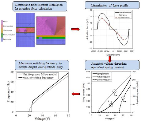
. The simulations are performed for conductive and dielectric liquids, using the applied voltages as boundary conditions: the voltage at the activated control electrode will be put at the applied voltage V. The voltages at the other control electrodes in the bottom layer and at the ground electrode are set to 0 V. In a quasi-static approach, the electrostatic actuation force is calculated from the computed electrostatic energy in Equation (2) at each droplet position. The electrostatic simulations are performed using 2D and 3D finite element models. For all simulations, a grid sensitivity analysis is performed to ensure a grid independent solution. The result of the grid sensitivity analysis indicates the number of cells and the required dimension of the cells. For the 2D case, the number of cells is typically in the order of 30,000 cells. In the case of a 3D simulation, the grid consists of around 250,000 elements. Figure 1 shows an example of a grid 2D electrostatic simulation.
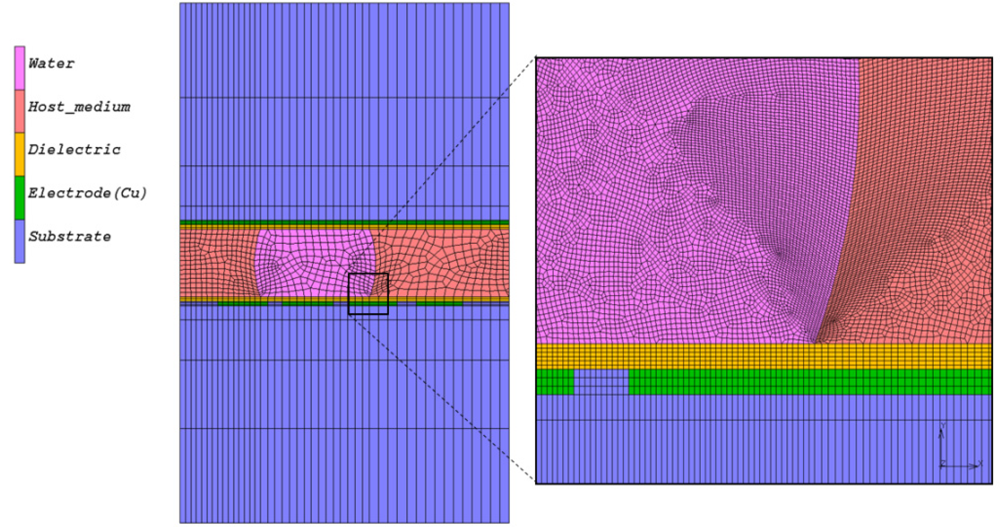
Figure 1. Example of a grid used in a 2D electrostatic simulation (left). Detail of the refined mesh around the three-phase line where high gradients in the electric field are expected (right).
Micromachines 03 00150 g001
The shear force Fw between the droplet and channel can be estimated when the velocity profile in the channel is known. A velocity profile can be assumed in the droplet with zero slip boundary conditions on top and bottom walls. Detailed simulations of the fluid flow inside the droplet show that a parabolic velocity profile is observed across the height of the channel if a no-slip boundary condition at the top and bottom wall is assumed [22]. Based on the average droplet velocity Uav, the vertical velocity profile in the channel can be determined. The geometrical properties of the system are as follows: Rc is the radius of the contact line circle and H is the gap between the top and bottom wall. The opposing forces can now be expressed as a function of the geometry of the droplet in the considered system. Assuming a parabolic velocity profile in the channel, the total shear force exerted by the top and bottom can be written as follows:
Micromachines 03 00150 i004   (4)
where μ is the droplet viscosity and A is the contact area between the droplet and the wall, v is the velocity profile parallel to the wall and y is the distance perpendicular to the wall.
Assuming that a droplet is moving through the filler fluid as a rigid body, the viscous drag force FD on the droplet can be estimated by:
Micromachines 03 00150 i005   (5)
where, CD is the drag coefficient and ρf is the density of filler fluid and Ac is the cross section area. The situation of a droplet moving through the filler fluid can be approximated by a cylinder in cross flow for the calculation of the drag coefficient. The drag coefficient CD depends on the Reynolds number of the flow. For a low Re number, which is the case in an electrowetting induced droplet flow, the drag coefficient CD is inversely proportional to the Reynolds number for the filler liquid and proportional to a constant a, depending on the geometry of the object. In the case of a sphere, a is 24. For a cylinder, a can be assumed to be 12. To estimate the drag coefficient on the droplet, a value between the sphere and cylinder case is chosen. As a result, the viscous drag force FD will scale linearly with the droplet velocity and can be written as follows:
Micromachines 03 00150 i006   (6)
In the case of air as a filler medium, the drag force is negligible compared to the dynamic contact line friction force and the viscous force.
The contact line friction force FCL originates from intermolecular attraction forces near the contact line of the droplet on the solid surface. Many different approaches exist to account for this effect, ranging from experimental empirical correlations [28,30,31] to complex molecular-kinetics modeling [32]. An excellent review of recent theoretical, experimental and numerical progress in the description of moving contact line dynamics can be found in [33]. In the work presented in this paper, an approximation for the static and the dynamic contact line friction force is used, for which the coefficients are experimentally determined. A dedicated test fixture is designed and fabricated to perform tilt tests for a droplet confined between two parallel surfaces. During the tilting of the fixture, the advancing and receding contact angle and the positions of the droplet interface (in the case of droplet motion) and the tilt angle required to initiate droplet movement between two parallel Teflon coated surfaces were studied (Figure 2). The gravitational force for this tilt angle corresponds to the static contact line friction. This also corresponds to the maximal static contact angle hysteresis. For a higher force, the contact angle hysteresis will not increase any more and the droplet will start moving. From the experimental results, the maximum static contact angle hysteresis factor [cos(θR) - cos θA]max can be experimentally determined as a function of the droplet volume, the channel height and the surface. In Figure 3(a), an image of the droplet during the tilt test is shown, indicating the advancing and receding contact angles. Figure 3(b) shows the evolution of the contact angles as a function of the tilt angle in the regime where the gravitational force is smaller than the contact line friction force. The expression for this static contact line friction force is [34]:
Micromachines 03 00150 i007   (7)
where w is the width of the drop in the direction perpendicular to the droplet motion, θA and θR are the advancing angle and the receding angle respectively and k is a constant depending on the shape of the droplet contact line.
Figure 2. Picture of the confined droplet between two Teflon coated surfaces during a tilt test (a). Evolution of the advancing and receding contact angle as a function of the tilt angle (b).
Micromachines 03 00150 g002
Figure 3. Measurement data for the evolution of the advancing and receding contact angle (a) and the total contact line friction force (b) as a function of the droplet velocity for a moving, confined droplet between two Teflon surfaces.
Micromachines 03 00150 g003
In the dynamic case, these contact angles are a function of the velocity of the moving contact line UCL. The left hand side of Figure 3 shows the evolution of the contact angles θA and θR as a function of the velocity. Since the contact line friction force depends on θA and θR, the friction force will also be a function of the velocity. Different algebraic expressions are presented in literature to approximate this dynamic behavior of the friction force. A commonly used expression based on the molecular interaction theory from [32] describes the dynamic part of the friction force as a power law function of the velocity:
Micromachines 03 00150 i008   (8)
where L is the length of the contact line and ζ is the coefficient of contact line friction defined in molecular kinetics and the exponent n varies between 0 and 2 [35]. Ren et al. [26] and Chen et al. [36] assume a linear relation between the friction and the velocity (i.e., n = 1) and extract the value of the coefficient of contact line friction ζ from a fitting of simulations of steady state velocities as a function of the applied voltage to experiments. This correlation is used to describe the dynamic contact line force: it is found that the coefficient of contact line friction ζ is 0.08 ± 0.03 Pa∙s. Figure 3 shows the measurements result of the advancing and receding contact angle (left) and the dynamic contact line friction (right) respectively as a function of the droplet velocity. The total contact line friction force for a droplet between two parallel surfaces can be written as a function of the droplet velocity:
Micromachines 03 00150 i009   (9)
with Rc the radius of the contact line and the droplet width w = 2Rc. For an actuation force smaller than the threshold force, the actuation force is compensated for by static contact line friction force, due to the droplet deformation. When the actuation force is high enough to overcome the threshold value of the static contact line friction force the droplet will start moving. Even for an increasing actuation force, the static contact line friction force is assumed to remain equal to the threshold force.

2.1.2. Summary for the Model Formulation

In the case of the actuation force being smaller than the threshold force, the static contact line friction force is equal to the actuation force and, as a result, the droplet will not move. The contact line force created by the droplet deformation will compensate for the actuation force on the droplet. Below the threshold force, the relation between the droplet deformation and the actuation force is given by Equation (8). For actuation forces higher than the threshold force, the droplet will move. For this dynamic case, the droplet motion can be described by Equation (1) using the description of the forces above:
Micromachines 03 00150 i010   (10)
The electrostatic actuation force is calculated by using finite element simulations. This force is calculated as a function of the applied voltage, the droplet volume, the electrode geometry (pitch and gap), the height of the channel or channel diameter, the dielectric constant and thickness of the insulation layer and the contact angle. Table 1 provides an overview of the independent parameters that are included in the dynamic model and a typical value used in the test case.
Table 1. Overview of the dynamic model parameters and the reference values used in the test cases.
CategoryDescriptionSymbolPlanar
GeometricalDroplet volumeVol2.7 μL
Channel height/diameterH/D1 mm
Electrode pitchwe + ge1 mm
Electrode gapge100 μm
Drag coefficientCd30
Insulation thicknesst1 μm
Material propertiesDroplet viscosityμd1.005 Pa∙s
Droplet densityρ1,000 kg/m3
Surface tensionγ72 Mn/m
Contact line friction (static)[cos( θR) - cos θA]max,st.~8 μN
Contact line friction coeff.ζ0.08 Ns/m2
Contact angleθ110°
Dielectric const. insulationεr3
ApplicationVoltageV45 V
Start positionx0−1 mm
Switching frequencyf25 Hz

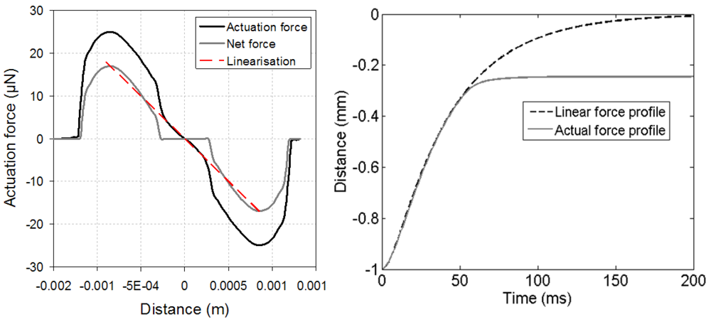
2.2. Model Linearization

The behavior of a moving droplet towards an activated electrode in the case of a sufficiently high actuation force Fel > FCL,static can be described as a damped mass-spring system. This simplified model can be used to develop a control strategy for the switching of the electrodes. The dynamic contact line friction, the drag force and the viscous dissipation force are proportional to the droplet velocity and can be described with an equivalent viscous damping coefficient ceq (Ns/m). The net actuation force Fel can be linearized in the region of the centre of the activated electrode and therefore be represented by an equivalent spring constant keq (N/m). The equivalent damping coefficient can be obtained from linearization of the function of the net actuation force as a function of the droplet position. This linearization can be derived from the analytical formulation of the actuation force. Such analytical descriptions can be found in [26,27,31]. In this paper, the linearization is numerically derived from a response surface model (RSM) that is fitted to a large design of experiments (DOE) of electrostatic simulations performed for the parameters listed in Table 1. The equivalent damping coefficient is
Micromachines 03 00150 i011   (11)
After linearization of the force profile, the droplet motion equation for a moving droplet in Equation (10), can be written as an equivalent equation of a damped spring-mass system:
Micromachines 03 00150 i012   (12)
Figure 4(left) shows the actuation force as a function of the droplet position for the parameters in Table 1 and an actuation voltage of 45 V. The net force acting on a moving droplet is approximated by the difference of the actuation force and the static contact line friction force. For droplet positions with an actuation force lower than the threshold force, the net actuation force is considered to be 0. In the region around the electrode centre, the net force can be linearized using an equivalent spring constant. The linearization is shown in Figure 4(left) as a dashed line. Figure 4(right) shows the comparison of the droplet motion calculated with the actual force profile and the equivalent linearized force profile.
Figure 4. Force profile as a function of the droplet position for an actuation voltage of 45 V: actual calculated profile (solid black line), difference between the actuation force and the static contact line friction (solid grey line) and the linearized force profile (dashed line).
Micromachines 03 00150 g004
Based on the nature of the motion equation, the droplet motion can exhibit oscillatory behavior. The linearized equation allows analysis of the droplet motion by calculation of an equivalent natural angular frequency ω0 and an equivalent damping ratio ζeq. In this way, the possible oscillatory behavior can be predicted and an optimal switching frequency for droplet motion over several subsequent electrodes can be obtained. The undamped angular frequency ω0, the damping ratio ζeq and the damped natural frequency ωd are defined as:
Micromachines 03 00150 i013   (13)
Figure 5. Force profile as a function of the droplet position for an actuation voltage of 45 V: actual calculated profile (solid black line), difference between the actuation force and the static contact line friction (solid grey line) and the linearized force profile (dashed line).
Micromachines 03 00150 g005
The value of the equivalent damping ratio ζeq determines the behavior of the droplet motion. For ζeq > 1, the system is overdamped and the droplet moves towards the electrode centre without oscillations. For ζeq = 1, the system is critically damped. For ζeq < 1, the system is underdamped, and the system oscillates with a damped natural frequency ωd. In the case of the electrostatically actuated droplet, the natural frequency and damping ratio depend on the actuation voltage for a certain configuration (system and material parameters). A certain voltage corresponds to a critical damped droplet behavior ζeq = 1. For lower voltages, the droplet motion will exhibit overdamped behavior and for higher voltages, oscillations will occur (Figure 5).

2.3. Model Limitations

The validity of the dynamic model is limited to a certain range of the system parameters. For parameter values outside this range, the dynamic model can no longer be used to accurately predict the droplet motion. Firstly, the application of the dynamic model is only valid for sufficiently small droplet volumes. The force calculations are performed for a certain droplet shape, assuming that the effect of surface tension dominates the effect of the gravity. For large droplet volumes, the droplet shape is flattened, due to the increased importance of the gravity. The characteristic length to assess the relative impact of the surface tension and the gravity is the capillary length λc. The capillary length is defined as follows:
Micromachines 03 00150 i014   (14)
In the case of a water droplet at 20 °C in air, the capillary length is around 2.7 mm. For droplets with dimensions smaller than the capillary length, surface tension dominates. For dimensions larger than the capillary length, gravity will have an impact on the droplet shape and the dynamic model cannot be used any more to predict the transient droplet motion.
Secondly, the dynamic model cannot be used for very high actuation voltages. The first reason is the effect of voltage saturation of the electrowetting effect. Above a certain threshold voltage, an increase in voltage will not result in a further contact angle decrease and consequently a higher actuation force acting on the droplet. The saturation limit of the voltage depends on the material properties of the solid surface and the liquid. The dynamic model should be used below this saturation limit. The second voltage-related limitation is caused by the required rise time of the voltage signal. In the model, a step function of the voltage application is assumed. In reality, a finite rise time is required to reach the desired voltage. This rise time is not included in the dynamic model.

3. Droplet Motion and Control

3.1. Model Solution Strategy

The electrostatic actuation force is known as a function of the droplet position x(t), whereas the shear force, drag force and contact line friction force are a function of the velocity U(t). Since the velocity is the derivative of the position, the differential Equation (10) of the force balance of a moving droplet can be solved numerically by integrating with respect to time to find the position x(t) and velocity U(t) of the droplet. By introducing the switching scheme of the electrodes, time dependent information is added to the electrostatic force. From the finite element simulations, this force is known as a function of the droplet position with respect to the activated electrode. The switching scheme describes which electrode is activated at which time, and with which voltage applied. This is schematically shown in Figure 6 for an array of 3 electrodes. On the left hand side, the force profile is shown as a function of the droplet position for three consecutive electrodes. On the right hand side, the time dependent voltage application at the different electrodes is shown for a switching frequency f. This means that each of the electrodes is powered for a time 1/f. As a result, the actuation force acting on the droplet is not only a function of the droplet position but also of time. For the droplet position, the centre of electrode ‘1’ is used as a reference. As an example, the time dependent force Fel(x,t) for three consecutive power electrodes with frequency f, can be written as follows :
Micromachines 03 00150 i015   (15)
where Fel,i(x) is the actuation force as a function of the distance from the centre of activated electrode ‘i’. Using a similar method, the time dependent force can be described for any switching pattern, including multiple electrodes activated at the same time, using superposition of the different force profiles.
Figure 6. (a) Electrostatic actuation force profile as a function of the droplet position at three subsequent electrodes. (b) Schematic representation of the switching of the voltage in the actuation electrodes.
Micromachines 03 00150 g006

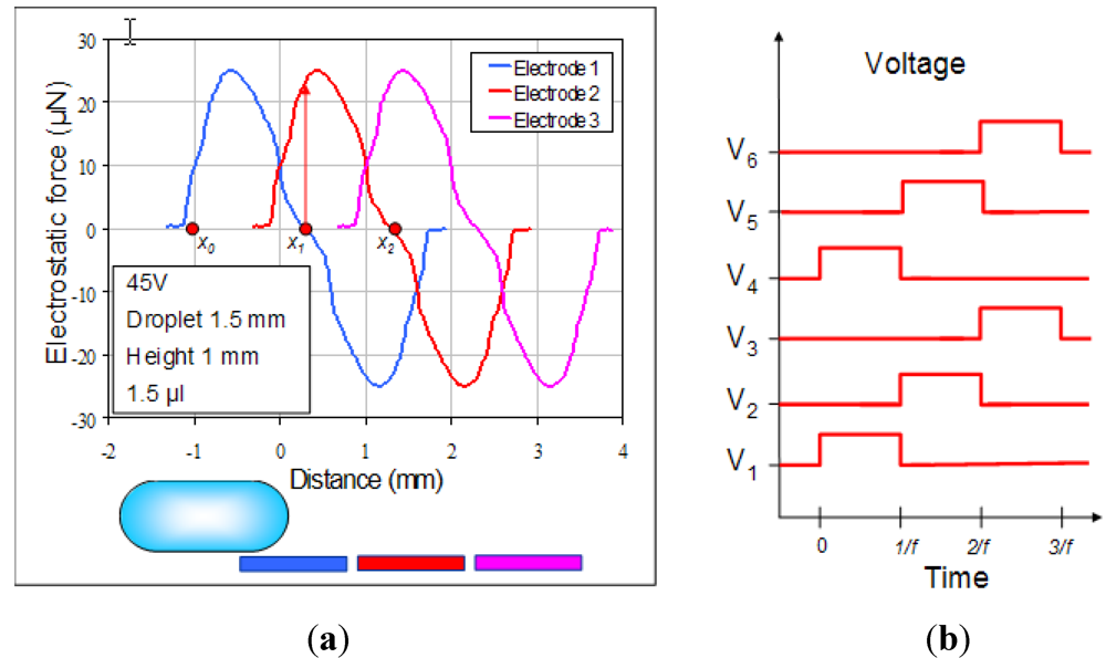
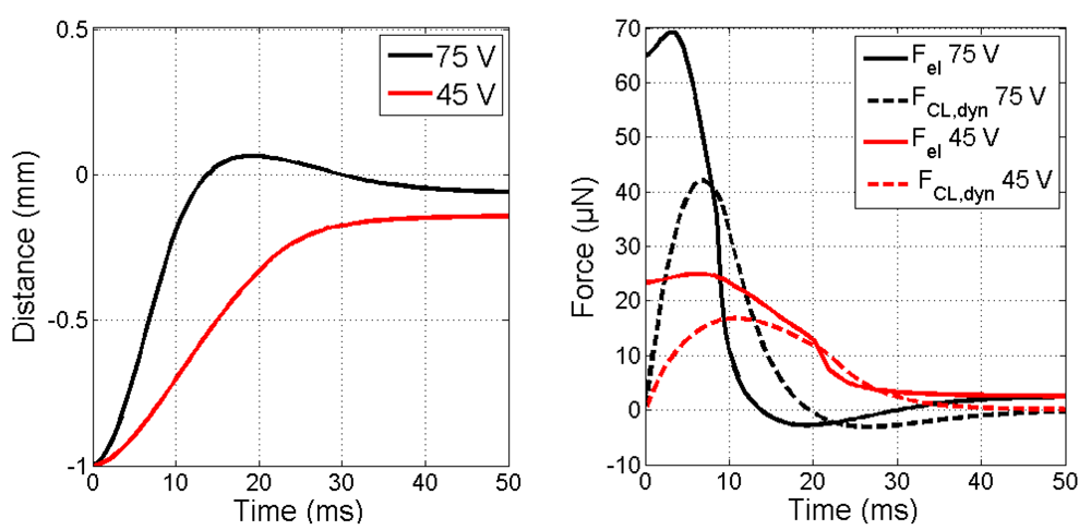
3.2. Single Electrode Response

In the considered test case, the electrode pitch is 1 mm, the electrode gap is 100 µm, the height of the channel is 1 mm and the droplet volume is 2.7 µL. First, the dynamic droplet motion of an individual droplet is calculated for a single activated electrode. A constant voltage is assumed to be applied to an electrode close to the droplet. This will be first illustrated for voltages of 45 V and 75 V. This can be considered an infinitely long voltage pulse. Even if the voltage is kept switched on, the droplet will stop at a position where the actuation force is lower than the opposing forces and the droplet does not have enough inertia to move on. The position after actuation depends on the applied voltage and the opposing forces. In this case, the force at the starting point is 22 µN. This is higher than the threshold force of 8 µN and therefore the droplet will start moving. As long as the net actuation force is higher than the opposing forces, the droplet will accelerate. When the opposing forces are higher than the actuation force the droplet will slow down and eventually stop. Depending on the opposing forces and applied voltage, this can mean that the droplet could stop before reaching the centre of the powered electrode if the voltage is too low (in the case of 45 V), or on the other hand that the droplet will overshoot the centre (in the case of 75 V). When the droplet overshoots the centre of the electrode, the droplet is pulled back towards the centre by the reverse electrostatic force. As a result, the droplet will perform an oscillation around the centre until its inertia is too small to overcome the opposing forces. The result is a damped oscillation around the centre of the powered electrode. The point where the droplet stops is important to ensure actuation by the next electrode in an array of subsequent electrodes. Figure 7 shows the first 50 ms of the results of the dynamic model for an applied voltage of 45 and 75 V. It can be observed that a minimal voltage required to actuate the droplet exists. At 18 V, the resulting electrostatic force is large enough to overcome the opposing force, however the net force is not sufficient to accelerate the droplet in such a way that the centre of the electrode is reached in a short time. In this case, after 100 ms only one quarter of the distance has been covered. This will have an influence on the switching frequency that can be achieved. To achieve a high flow rate, a switching frequency should be sufficiently high. Therefore, a higher actuation voltage might be required.
Figure 7. Results of the dynamic droplet position model for the parameters listed in Table 1 for the parallel plate test case for actuation voltages of 45 V and 75 V.
Micromachines 03 00150 g007

3.3. Droplet Trajectory over an Array of Electrodes

The purpose of the array of electrodes in the microfluidic system is to generate a continuous flow of discrete liquid droplets. To generate a continuous motion of the droplet through the channel, the droplet should be attracted from one electrode to the next by subsequently applying a voltage to the array of electrodes. This means that analysis for a single electrode can be repeated for all the electrodes in the array. What the droplet motion through the channel looks like, depends on the actuation voltage, the switching frequency, the starting position of the droplet and the opposing forces. The end position of the droplet motion for the first activated electrode is the starting position of the motion for the second actuated electrode. The droplet motion from one electrode to the next will be successful if the actuation force of the next electrode acting on the droplet is sufficiently high for the position the droplet is in at the moment. The voltage is switched off in the first electrode and switched on in the second. It is important to carefully control the switching frequency. If the frequency is set too high, the electrodes will switch before the droplet reaches the region of attraction of the next electrode and the droplet will stop. The safest option is to wait to switch until the droplet has stabilized. However, a successful droplet motion can be achieved by switching before this time at the right side of the oscillation. On the other hand, if the velocity is too low, the flow rate is suboptimal and the droplet will be waiting before being switched to the next electrode. In this case, the power consumption will be unnecessarily high. To develop an efficient control of the voltage and frequency of the droplet actuation, the transient droplet motion across multiple electrodes is studied more in detail. Figure 8 shows the transient droplet motion for the reference parameters during the actuation over three electrodes using a switching frequency of 20 Hz.
Figure 8. (a) Dynamic droplet response for the actuation over three subsequent electrodes for an actuation voltage of 40 V. (b) Evolution of the actuation and opposing force on the droplet as a function of time.
Micromachines 03 00150 g008

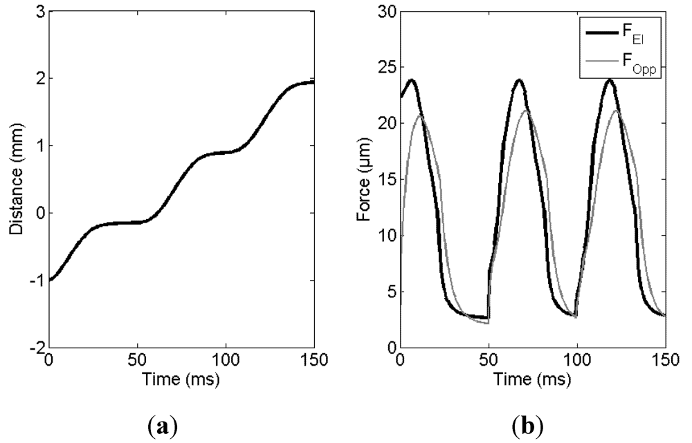
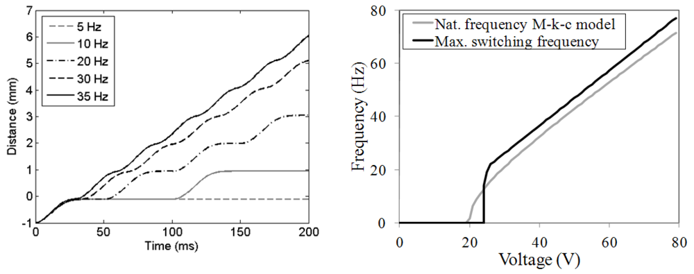
3.4. Influence of Switching Frequency

From the previous graphs, it could be observed that the chosen frequency is safe to actuate the droplet over that particular array of electrodes. However, it is also clear that there is still room for improvement to increase the flow rate for the same voltage by increasing the frequency. Figure 9(left) shows the effect of frequency on the droplet motion for a range of the frequency of 5 to 35 Hz for an actuation voltage of 40 V. In the graph, the first 200 ms of the motion is shown. This corresponds to one cycle for a frequency of 5 Hz. The droplet can follow the voltage switches up to a frequency of 35 Hz. For the case of 40 Hz, the droplet is too far away from the second electrode at the moment of switching and the droplet is stuck close to the center of the first electrode. Further study shows that the maximum switching frequency for this case with an actuation voltage of 40 V is 36 Hz. A maximum frequency can be determined for each actuation voltage. In the case of an actuation voltage of 60 V, the maximum switching frequency is 62 Hz. This is important information to develop an efficient and robust control for the droplet actuation. For each value of the actuation voltage, a maximum frequency can be found. Figure 9(right) shows the maximum frequency that can be used for successful droplet transportation over multiple electrodes for a voltage range of 0 to 80 V. The minimal voltage that is required to move the droplet is 18 V. However, for this actuation voltage the droplet does not reach the centre of the powered electrode. Simulations show that the minimal voltage for which droplet motion over multiple electrodes can be achieved is 28 V. For the range in between 18 and 28 V, the droplet will move but will not move far enough to be close enough to the second electrode. For voltages higher than 28 V, increasing frequencies can be reached for increasing actuation voltages. However, the voltage is limited by the dielectric breakdown in the insulating material. Therefore, a trade-off needs to be made between the voltage and frequency, considering the limitations of the insulating material, the specifications of the power supply and the complexity of control.
Figure 9. Maximum switching frequency as a function of the actuation voltage for the planar electrode configuration with air as filler liquid and with the system parameters listed in Table 1. The switching frequency is compared for the results of the dynamic model using the actual force profile and the results of the linearized damped spring-mass model (two times the natural frequency).
Micromachines 03 00150 g009
In Figure 9(right), the maximum switching frequency is compared to the double of the natural frequency of the linearized damped mass-spring model. In the linearized model, the mass moves from one extreme point to the opposite (Figure 4(left)). After one half of the period, the opposite position is reached. At this moment, the voltage can be switched to the next electrode to move the droplet forward towards this next electrode. Therefore, the optimal switching frequency, extracted from the linearized model, can be written as follows:
Micromachines 03 00150 i016   (16)
where ω0 is the angular natural frequency of the damped mass-spring system in Equation (13). By comparing the switching frequency to the maximum frequency obtained from the simulations with the actual force profile, two differences can be observed. The first difference is that the damped mass-spring system predicts a continuous droplet motion from one electrode to the next for a lower voltage than the actual force profile. For voltages higher than 18 V, a droplet motion is realized. For this moving droplet, using the linearized model, a natural frequency and consequently a switching frequency can be found. In reality however, the droplet will not move far enough to be actuated by the next electrode. Only for a voltage of minimum 25 V can continuous droplet motion be achieved. The second deviation between the linearized model and the actual force profile is that the linearized model underpredicts the value of the switching frequency. This can be explained by the fact that the actuation force on the droplet already starts acting before the droplet reaches the centre of the previous electrode. As a result, the voltage can be switched slightly before this position is reached, leading to a slightly higher achievable switching frequency. Despite those two deviations, the linearized model provides a useful approximation of the optimal switching frequency within 10% of the results obtained by the dynamic model using the actual force profile. Therefore, the linearized model can be used as a fast tool to develop a control strategy for the activation of the electrodes in order to optimize the droplet flow.

4. Conclusions

In this article, a general methodology for the dynamic modeling of electro-actuated droplets is presented to predict transient droplet motion. In this simplified approach, the droplet is dealt with as a single mass. The dynamic model predicts the macroscopic droplet motion, based on a force balance of all forces acting on the droplet. The opposing forces on the droplet are, as described, algebraic expressions as a function of the average droplet velocity. For the electrostatic actuation force, simulation results are used. Empirical models are derived from tilt tests of confined droplets to describe the contact line friction forces. Furthermore, a linearized equivalent damped mass—spring model has been derived to approximate the dynamic droplet motion. This linearized model can be used to develop control strategies for the switching of the electrodes.
Next, the methodology is applied to an array of electrodes. The voltage is switched subsequently from one electrode to the next. For each actuation voltage, a maximum switching frequency is found that the droplet will be able to follow. For higher frequencies, the droplet will not reach the next electrode before the voltage is switched. The maximal switching frequency can be approximated by twice the natural frequency of the linearized damped mass—spring system. Therefore, the linearized model can be used for the development of control strategies to optimize the switching of the electrodes. Using an optimized switching frequency, the dynamic model predicts droplet velocities in the range of 5 to 10 cm/s for a voltage range from 30 to 80 V.

References

  1. Mugele, F.; Baret, J.-C. Electrowetting: From basics to applications. J. Phys. Condens. Matter. 2005, 17, R705–R774. [Google Scholar] [CrossRef]
  2. De Gennes, P.-G.; Brochard-Wyart, F.; Quere, D. Capillarity and Wetting Phenomena; Springer: New York, NY, USA, 2004. [Google Scholar]
  3. Fouillet, Y.; Jary, D.; Chabrol, C.; Claustre, P.; Peponnet, C. Digital microfluidic design and optimization of classic and new fluidic functions for lab on a chip systems. Microfluid. Nanofluid. 2007, 4, 159–165. [Google Scholar]
  4. Pollack, M.G.; Shenderov, A.; Fair, R.B. Electrowetting-based actuation of droplets for integrated microfluidics. Lab Chip 2002, 2, 96–101. [Google Scholar] [CrossRef]
  5. Cho, S.K.; Moon, H.; Kim, C.J. Creating, transporting, cutting, and merging liquid droplets by electrowetting-based actuation for digital microfluidic circuits. J. Microelectromechan. Syst. 2003, 12, 70–80. [Google Scholar] [CrossRef]
  6. Chakrabarty, K.; Su, F. Digital Microfluidic Biochips: Synthesis, Testing, and Reconfiguration Technique; CRC Press: Boca Raton, FL, USA, 2006. [Google Scholar]
  7. Berge, B.; Peseux, J. Variable focal lens controlled by an external voltage: An application of electrowetting. Eur. Phys. J. E 2000, 3, 159–163. [Google Scholar] [CrossRef]
  8. Yang, S.; Krupenkin, T.N.; Mach, P.; Chandross, E.A. Tunable and latchable liquid microlens with photopolymerizable components. Adv. Mater. 2003, 15, 940–943. [Google Scholar] [CrossRef]
  9. Kuiper, S.; Hendriks, B.H.W. Variable-focus liquid lens for miniature cameras. Appl. Phys. Lett. 2004, 85, 1128–1130. [Google Scholar]
  10. Hayes, R.A.; Feenstra, B.J. Video-speed electronic paper based on electrowetting. Nature 2003, 425, 383–385. [Google Scholar]
  11. Heikenfeld, J.; Steckl, A.J. High-transmission electrowetting light valves. Appl. Phys. Lett. 2005. [Google Scholar] [CrossRef]
  12. Washizu, M. Electrostatic actuation of liquid droplets for microreactor applications. IEEE Trans. Ind. Appl. 1998, 34, 732–737. [Google Scholar] [CrossRef]
  13. Lee, J.; Kim, C.-J. Surface-tension-driven microactuation based on continuous electrowetting. J. Microelectromech. Syst. 2000, 9, 171–180. [Google Scholar] [CrossRef]
  14. Yun, K.S.; Cho, I.J.; Bu, J.U.; Kim, C.-J.; Yoon, E. A surface-tension driven micropump for low-voltage and low-power operations. J. Microelectromech. Syst. 2002, 11, 454–461. [Google Scholar] [CrossRef]
  15. Quilliet, C.; Berge, B. Electrowetting: A recent outbreak. Curr. Opin. Colloid Interface Sci. 2001, 6, 34–39. [Google Scholar] [CrossRef]
  16. Pamula, V.K.; Chakrabarty, K. Cooling of integrated circuits using droplet-based microfluidics. In Proceedings of the 13th ACM Great Lakes Symposium on VLSI 2003, Washington, DC, USA, 28–29 April 2003; pp. 84–87.
  17. Paik, P.Y.; Pamula, V.K.; Chakrabarty, K. Thermal effects on droplets transport in digital microfluidics with application to chip cooling. In Proceedings of theInter Society Conference on Thermal Phenomena, Las Vegas, NV, USA, 1–4 June 2004; pp. 649–654.
  18. Paik, P.Y.; Pamula, V.K.; Chakrabarty, K. Droplet-based hot spot cooling using topless digital microfluidics on a printed circuit board. In Proceedings of the IEEE International Workshop on Thermal Investigations of ICs and Systems, Belgirate, Italy, 27–30 September 2005; pp. 278–283.
  19. Mohseni, K. Effective cooling of integrated circuits using liquid alloy electrowetting. In Proceedings of the 21st Semi-Therm Symposium, San Jose, CA, USA, 15–17 March 2005; pp. 20–25.
  20. Nicole, C.; Lasance, C.J.M.; Prins, M.W.J.; Baret, J.-C.; Decre, M.M.J. A Cooling System for Electronic Substrates. WIPO Patent WO 2006/016293 A1, 16 February 2005. [Google Scholar]
  21. Garimella, S.V.; Bahadur, V. Electrowetting Based Heat Spreader. U.S. Patent 11/752702, 23 May 2007. [Google Scholar]
  22. Oprins, H.; Danneels, J.; van Ham, B.; Vandevelde, B.; Baelmans, M. Convection heat transfer in electrostatic actuated liquid droplets for electronics cooling. Microelectron. J. 2008, 39, 966–974. [Google Scholar] [CrossRef]
  23. Oprins, H.; Vandevelde, B.; Fiorini, P.; Beyne, E.; de Vos, J.; Majeed, B. Device for cooling integrated circuits. U.S. Patent 20110304987 A1, 1 June 2011. [Google Scholar]
  24. Oprins, H.; Fiorini, P.; de Vos, J.; Majeed, B.; Vandevelde, B.; Beyne, E. Modeling, design and fabrication of a novel electrostatically actuated droplet based impingement cooler. In Proceedings of the 10th PowerMEMS, Leuven, Belgium, 30 November–3 December 2010; pp. 191–194.
  25. Majeed, B.; Jones, B.; Oprins, H.; Vandevelde, B.; Sabuncogolu, D.; Fiorini, P. Fabrication of an electrostatically actuated impingement cooling device. In Proceedings of the 44th International Symposium on Microelectronics, Long Beach, CA, USA, 9–13 October 2011.
  26. Ren, H.; Fair, R.B.; Pollack, M.G.; Schayghnessy, E.J. Dynamics of electrowetting droplet transport. Sens. Actuat. B 2002, 87, 201–206. [Google Scholar] [CrossRef]
  27. Bahadur, V.; Garimella, S.V. An energy-based model for electrowetting-induced droplet actuation. J. Micromech. Microeng. 2006, 16, 1494–1503. [Google Scholar] [CrossRef]
  28. Ren, H.; Fair, R.B.; Pollack, M.G. Automated on-chip droplet dispensing with volume control by electro-wetting actuation and capacitance metering. Sens. Actuat. B 2004, 98, 319–327. [Google Scholar] [CrossRef]
  29. Berthier, J.; Dubois, P.; Clementz, P.; Claustre, P.; Peponnet, C.; Fouillet, Y. Actuation potentials and capillary forces in electrowetting based microsystems. Sens. Actuat. A 2007, 134, 471–479. [Google Scholar] [CrossRef]
  30. Shapiro, B.; Moon, H.; Garrell, R.L.; Kim, C.-J. Equilibrium behaviour of sessile drops under surface tension, applied external fields, and material variations. J. Appl. Phys. 2003, 93, 5794–5811. [Google Scholar] [CrossRef]
  31. Mohseni, K.; Baird, E. Digitized heat transfer using electrowetting on dielectric. Nanoscale Microscale Thermophys. Eng. 2007, 11, 99–120. [Google Scholar] [CrossRef]
  32. Blake, T.D. The physics of moving wetting lines. J. Colloid Interface Sci. 2006, 299, 1–13. [Google Scholar] [CrossRef]
  33. Bonn, D.; Eggers, J.; Indekeu, J.; Meunier, J.; Rolley, E. Wetting and spreading. Rev. Mod. Phys. 2009, 81, 739–805. [Google Scholar] [CrossRef]
  34. Extrand, C.W.; Kumagai, Y. Liquid drops on an inclined plane: The relation between contact angles, drop shape and retentive force. J. Colloid Interface Sci. 1995, 170, 515–521. [Google Scholar] [CrossRef]
  35. Chen, J.H.; Hsieh, W.H. Electrowetting-induced capillary flow in a parallel-plate channel. J. Colloid Interface Sci. 2006, 296, 276–283. [Google Scholar] [CrossRef]
  36. Chen, N.; Kuhl, T.; Tadmor, R.; Lin, Q.; Israelachvili, J. Large deformations during the coalescence of fluid interfaces. Phys. Rev. Lett. 2004. [Google Scholar] [CrossRef]

