3.1. Comparisons between SGM and SHM
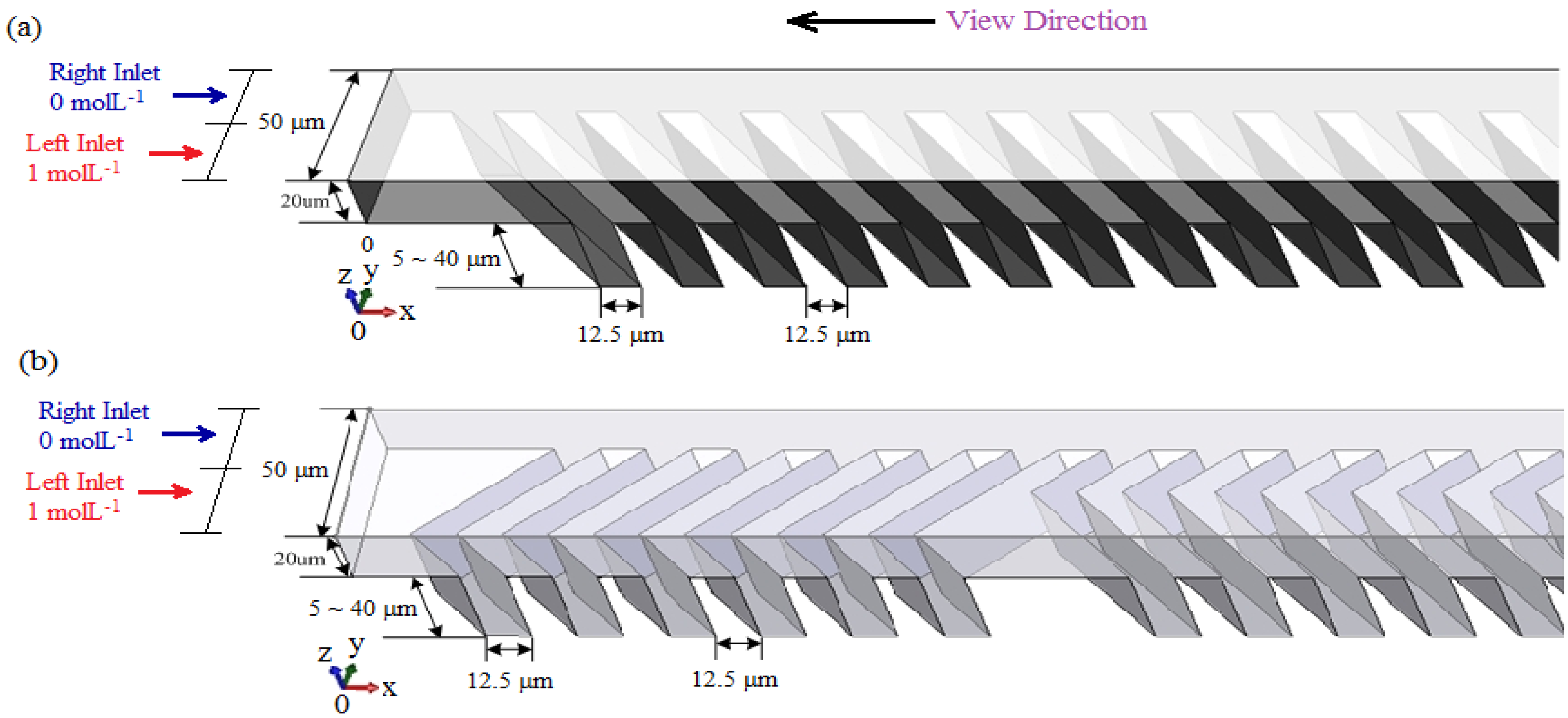
For simplicity of discussion, a specific micromixer is represented by the type of micromixer followed by the numerical value of its groove depth. For example, SGM 5 represents a SGM with groove depth at 5 μm, and SHM 10 represents a SHM with groove depth at 10 μm. To compare mixing processes in SGM and SHM, we first took SGM 10 and SHM 10 as examples.
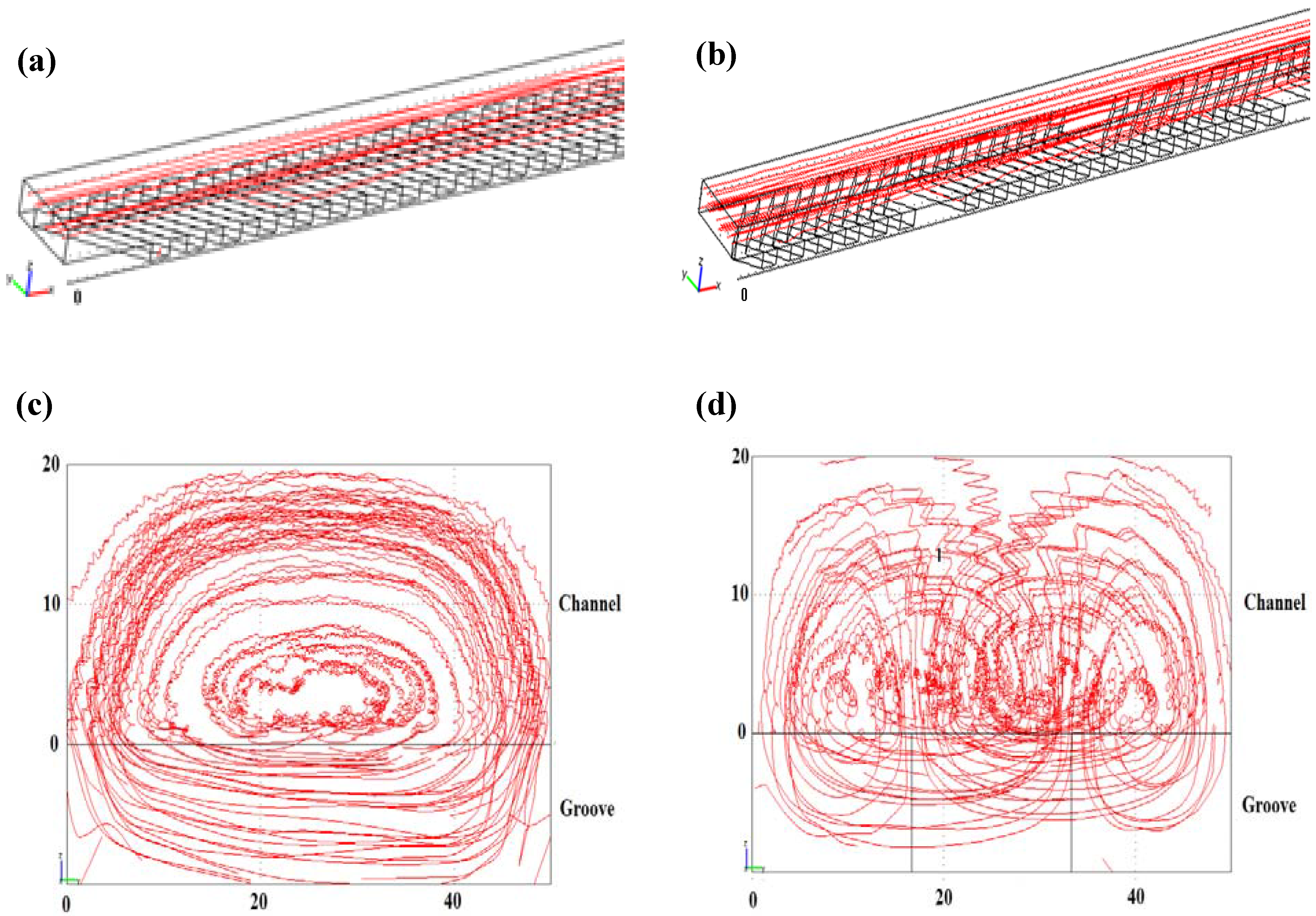
In principle, concentration-based analysis is the most reliable method in studying molecular micromixing because every aspect of the mixing process, such as bulk advection and molecular diffusion, will eventually be reflected in changes in concentration. The velocity field in SGM and SHM, as shown in
Figure 2, can be helpful to understand the concentration change in a microchannel. In a steady flow, the streamlines coincide with the particle traces and the velocity vectors are tangent to the streamlines at all points [
19]. As seen from the cross-section streamlines in
Figure 2(c) and (d), there is only one overall helical flow in the SGM while two helical flows exist in the SHM. This is in good agreement with other reports in literature [
19,
21]. Before mixing, the fluids at two inlets had concentrations of 1 mmol/L and 0 mmol/L, respectively. With the rotation motions of the helical flow caused by either one vortex in SGM or two vortices in SHM to transport mass (thus mixing two fluids of two concentrations to be mixed), two completely different concentration profiles within the channels would result. Therefore, as the vortex flows transport masses to be mixed within a cross section and along the channels—before the fluids are completely mixed—one can imagine that the concentration of a specific point within a cross section will be different (either higher or lower) from that of the same point but at another cross section along the channel. The oscillations appear in the concentration
vs. channel length profiles.
To study the mixing mechanics in SGM and SHM, we compared their concentration profiles, as shown in
Figure 3.
Figure 2.
Streamlines of velocity fields in (a), (c) SGM and (b), (d) SHM. (a), (b), 3D view. (c), (d), y-z plane viewed from inlet.
Figure 2.
Streamlines of velocity fields in (a), (c) SGM and (b), (d) SHM. (a), (b), 3D view. (c), (d), y-z plane viewed from inlet.
Figure 3.
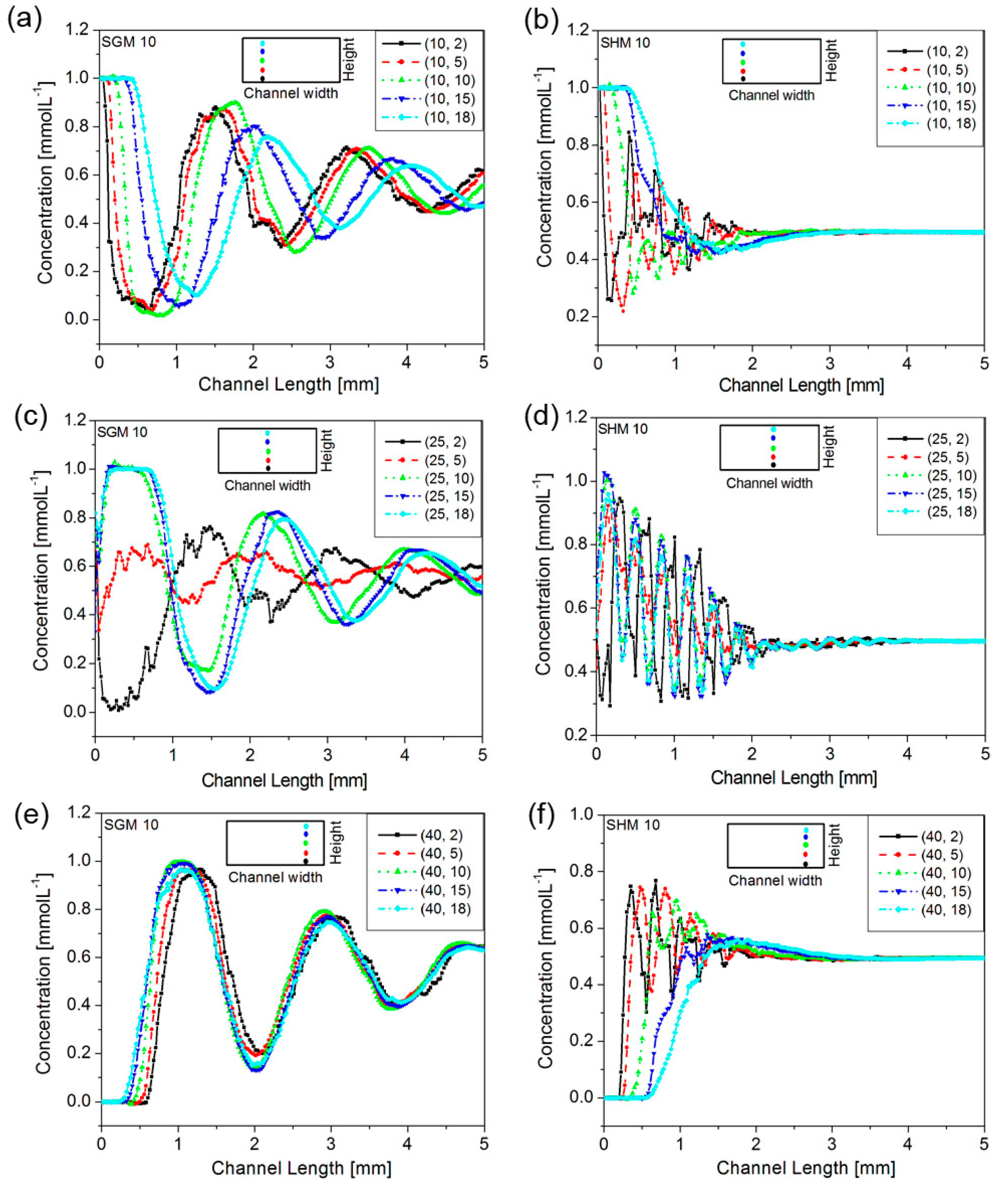
Concentration profiles within SGM 10 (a, c, e) and SHM 10 (b, d, f) along the channel length (in x-direction) (unit in mm). The concentration data were collected in the y–z coordinate system of the channel cross section with its bottom-left set as the origin (0, 0) (unit in μm). Channel dimension: 20 (h) × 50 (w) μm; groove dimension: 12.5 (w) × 10 (d) μm.
Figure 3.
Concentration profiles within SGM 10 (a, c, e) and SHM 10 (b, d, f) along the channel length (in x-direction) (unit in mm). The concentration data were collected in the y–z coordinate system of the channel cross section with its bottom-left set as the origin (0, 0) (unit in μm). Channel dimension: 20 (h) × 50 (w) μm; groove dimension: 12.5 (w) × 10 (d) μm.
As generally discussed in the literature, a helical flow is created inside the microchannel of SGM due to a down-channel flow component as well as transversely rotational flow component [
10,
19,
30]. All concentration profiles of SGM, as seen in
Figure 3(a), (c) and (e), showed that the concentrations oscillated along the channel length as the two mixing fluids travelled helically and mixed along the channel length. In addition, these oscillations showed, in comparison with those in SHM, nearly the same amplitudes, larger peak-to-peak pitches and slower concentration convergences to the expected concentration. This suggests that the single helical flow causes the concentration change at each cross-section location and that the overall mixing in SGM is coarse and slow. The concentration profiles collected at the middle of the SGM channel cross-section, as shown in
Figure 3(c) were of particular interest. In this case, the concentrations at locations close to the grooves first decreased, likely due to the first arrival of low-concentration fluid from the right inlet (cf.
Figure 1 for viewing directions); conversely, the concentrations at locations further away from the grooves first increased, likely due to the first arrival of high-concentration fluid from the left inlet. This observation further confirms that a clockwise (depending on the orientation of the grooves) helical flow is created in SGM mixers along the channel length to promote mixing. This is in good agreement with the results obtained by particle tracking method in the literature [
19].
In the case of the SHM, one large clockwise vortex was created at long arms of the grooves, and one small counter-clockwise vortex was created at short arms of the grooves. These two transverse vortices changed periodically with the alternation of the asymmetry of structure and produced substantial oscillations and faster concentration convergence in the concentration profiles, as shown in
Figure 3(b), (d) and (f). This clearly suggests that, in comparison with SGM, SHM enables finer (
i.e., more frequent) and faster mixing for the given flow rate investigated. Moreover, as seen from
Figure 3(b) and
Figure 3(f), the oscillations were more violent and with larger amplitudes at locations near the grooves; in contrast, the oscillations were delayed and less vigorous at locations further away from the grooves. These observations strongly indicate that the initial chaotic mixing in SHM is only limited to the regions close to the grooves until the upper portion of the channel fluid is sufficiently affected by the two opposing vortices. Since the two mixing fluids are first turned clockwise and then counter-clockwise by two vortices, the interface of two fluids (not the interface of two vortices) remains in the middle of the channel [
12]. As the concentrations at the middle of the channel cross-section are always controlled by the large vortex, either left-positioned (high concentration) or right-positioned (low concentration), the concentration profiles at the middle of the channel cross-section, showed substantial oscillations at all times until mixing completed, as shown in
Figure 3(d).
Since the groove depth has been shown to be one of the most effective parameters to affect mixing efficiency [
31,
32], we compared the effect of groove depth on the mixing performance in both SGM and SHM. As shown in
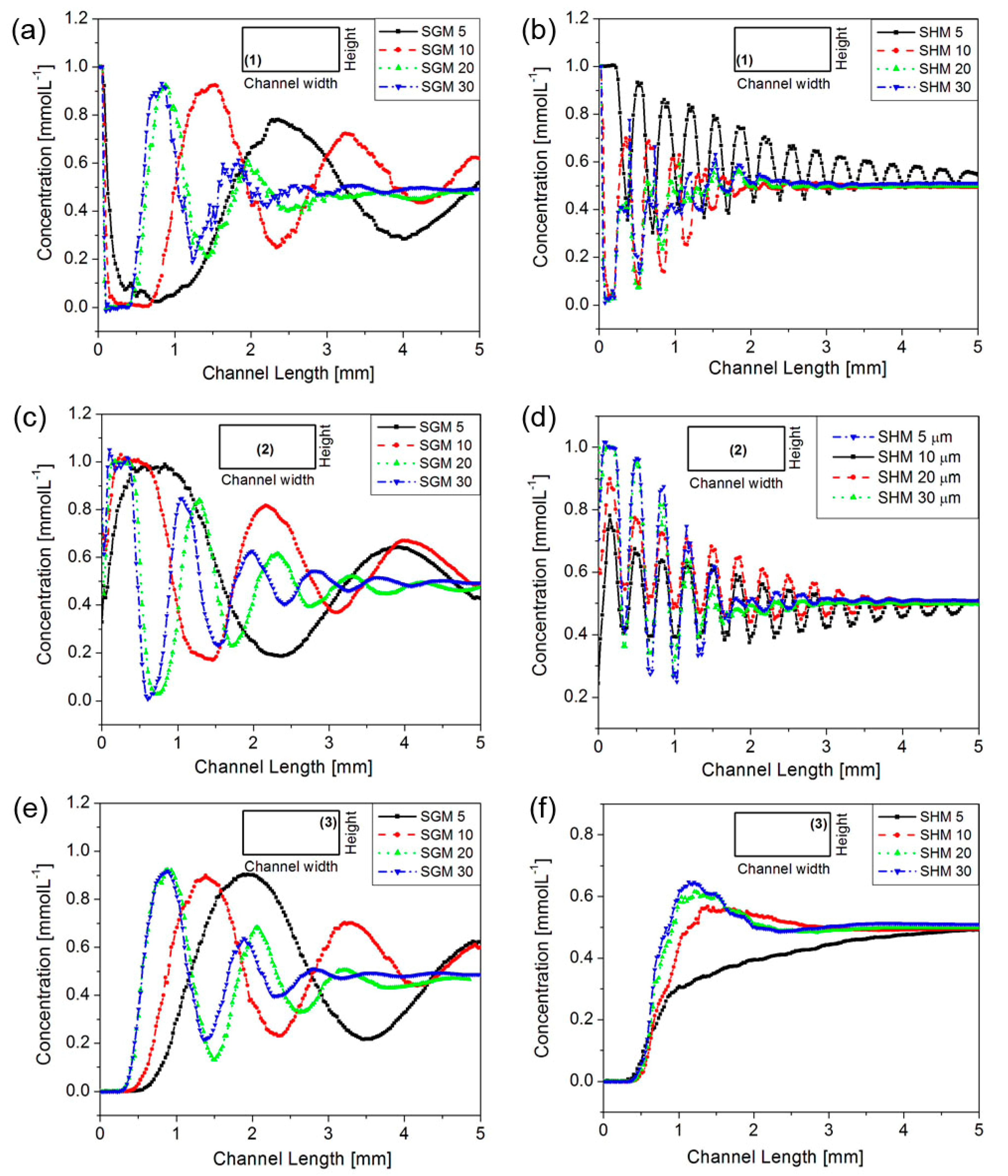
Figure 4, the concentration data were collected at three different representative cross-section locations. At Location (1) which is near the grooves, all concentration profiles in both SGM and SHM showed increased initial slopes—concentration changed faster for a given mixing length in the channels—as groove depth increased from 5 μm to 30 μm, suggesting that mixing was significantly improved as the groove became deeper. This is in good agreement with a previously reported observation [
25]. Comparing
Figure 4(a) with
Figure 4(b), it is evident that the concentration oscillations in the SHMs were more frequent than those in the SGMs and therefore the pitches of the SHM were much smaller than those of the SGM; this is likely a indication of a more active mixing in the SHM than in the SGM under the same fluidic conditions. As a result, the SHM demonstrated a significantly faster concentration convergence to the perfectly mixed value than the SGM at a given groove depth, as shown in
Figure 4(a) and (b). This trend became more significant with increased groove depths. Likewise, the concentration profiles of the center-point of the mixers, both the SGM and the SHM, are shown in
Figure 4(c) and
Figure 4(d), respectively. As expected, the average pitches of SGM decreased with increasing groove depth, indicating more effective mixing efficiency due to increased groove depth. Interestingly, pitches of the SHM remained the same regardless of the groove depth, and the pitch length was consistent with the channel length occupied by one full SHM structure cycle, indicating the full helical-flow cycle was
only related to the structures in SHM. This observation was also noted in
Figure 4(b). Like at Locations (1) and (2), similar mixing dependence on groove depth in SGM was observed at Location (3), a location further away from the grooves, as shown in
Figure 4(e). However, in the case of SHM, as shown in
Figure 4(f), the concentration streamlines showed small concentration oscillations before converging to the final concentration for all the groove depths investigated in this study. This strongly suggests that mixing by the two opposing vortices is less effective in the SHM at locations far away from the groove. This is in sharp contrast with the SGM of which the concentration streamlines showed less location dependence.
Nevertheless, based on the above discussion, we conclude that deep grooves are in favor of the chaotic mixing in both SGM and SHM and that the mixing is improved as the depth of the groove increases, as also described in previous reports [
8,
11,
25].
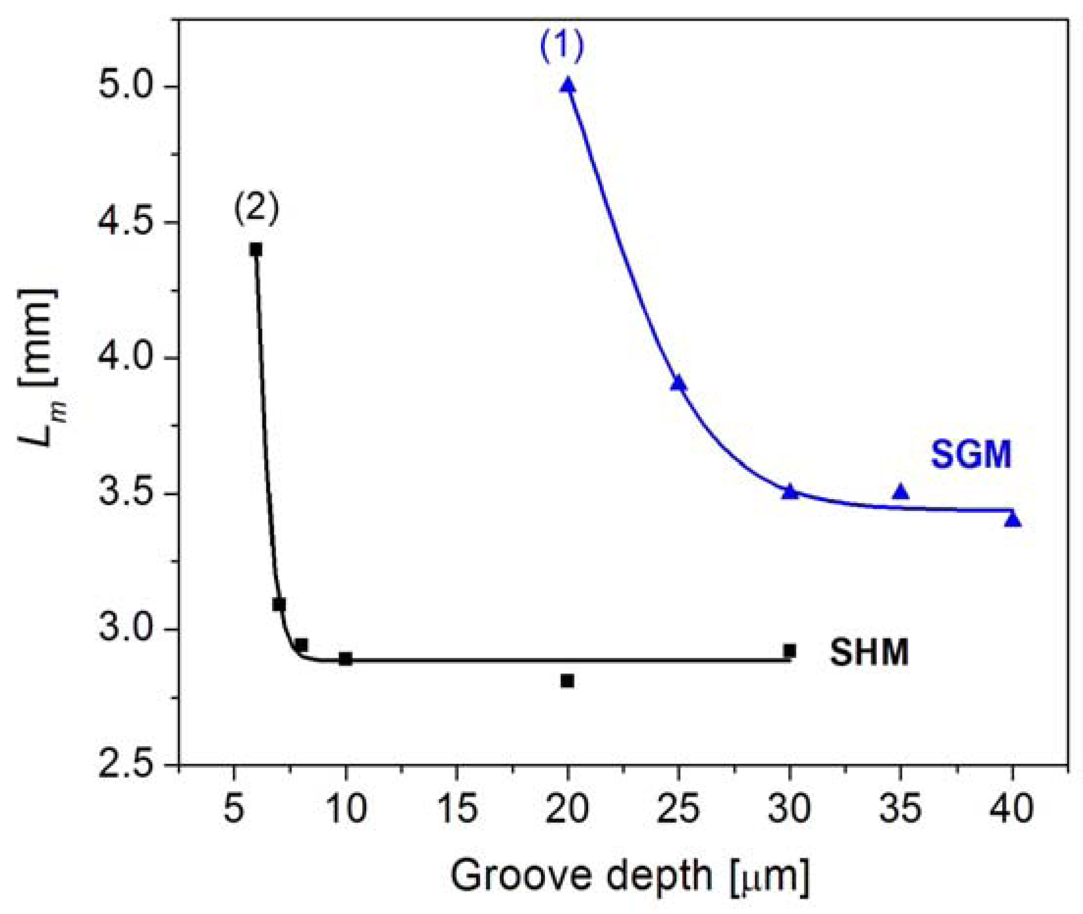
From the concentration profiles, mixing completion length, Lm, can be easily calculated. Defined as the channel length needed to achieve a concentration value of C = 0.5 ± ε mol/L where ε is an assigned small value called mixing extent depending to specific application requirements. The Lm is the most straightforward parameter to characterize the mixing performance as a small Lm value corresponds to an efficient mixing.
We compared the effects of groove depth on the
Lm at a specific
ε = 0.01 for both SGM and SHM. As shown in
Figure 5, both lines first fell sharply and then leveled off with further increased groove depths, indicating that deepening groove within a certain range was effective in enhancing the mixing, and any further increase in groove depth beyond a threshold was ineffective. More specifically, for SGM as shown of Line (1) of
Figure 5,
Lm values (while keeping
ε = 0.01) decreased from 5 mm to 3.5 mm as the SGM groove depths increased from 20 μm to 30 μm. When the groove depths were further increased from 30 to 40 μm, the
Lm remained almost constant at ~3.5 mm. For the SHM, as shown of Line (2) of
Figure 5, mixing was significantly enhanced when groove depths were increased from 6 μm to 8 μm. However, when the SHM groove depths were further increased from 10 to 30 μm, the dependence of
Lm on groove depth was insignificant. This result confirms the notion that a deeper groove does not always lead to a better mixing, as suggested by Aubin
et al. who observed that a maximum groove depth existed whereby decrease in the maximum striation thickness was no longer significantly improved [
23]. The reason for this to happen is that very deep grooves may also bring a significant negative contribution that would offset their positive effect on mixing. It is known that the groove-caused transverse fluid transportation within a microchannel simultaneously happens above the grooved floor and under the floor (
i.e., within the grooves). Those flowing above the floor are mostly in the vortices and experience a fast chaotic mixing, and those flowing within the grooves are basically in a typical laminar flow and are mostly exposed to a slow diffusion-dominated mixing. When the groove depth is overly increased, a large quantity of fluid enters the grooves and its slow mixing becomes significant to the overall mixing within the channel. The explanation is also in good agreement with the results reported in the literature that deep wells had a large dead volume which increased the residence time of the sample within the wells [
10]. Furthermore, it is evident that at the same groove depth, a much smaller
Lm value is needed for the SHM than the SGM, confirming that mixing within the SHM is more effective and faster than that within the SGM. This is consistent with reported simulation and experimental results [
11,
12].
Figure 4.
Concentration profiles in SGM (a, c, e) and SHM (b, d, f) with different groove depths. The concentration data were collected along channel length in its flow direction at the fixed cross-section locations represented by Location (1) at (5, 3) (coordinate units in μm), Location (2) at (25, 10), and Location (3) at (45, 17) in the y–z coordinate system of the channel cross section with its bottom-left point set as origin (0, 0). Channel dimension: 20 (h) μm × 50 (w) μm; groove width, 12.5 μm.
Figure 5.
Effects of groove depths on Lm in SGM and SHM. Note that Lm simulation results did not converge for the mixing extent of ε = 0.01 within the simulated 5-mm channel length when the groove depths were less than 20 μm for SGM and 5 μm for SHM.
Figure 5.
Effects of groove depths on Lm in SGM and SHM. Note that Lm simulation results did not converge for the mixing extent of ε = 0.01 within the simulated 5-mm channel length when the groove depths were less than 20 μm for SGM and 5 μm for SHM.
3.2. Hybrid floor-grooved micromixers
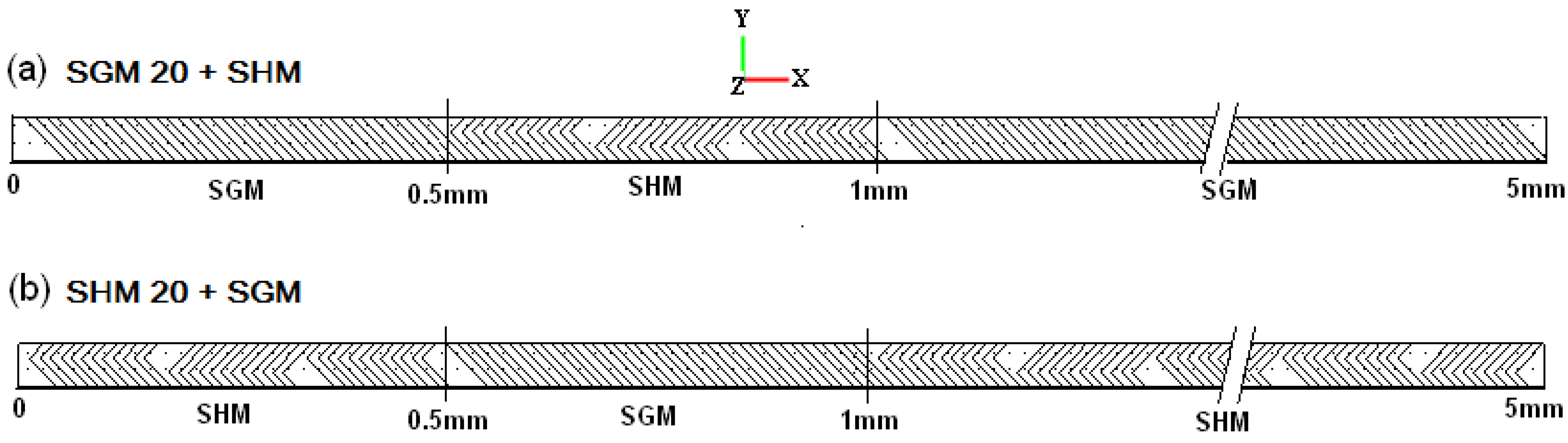
As has been clearly illustrated above, both the SGM and SHM mix different fluids via different mechanisms, and factors influencing their mixing efficiencies also work differently on the two different types of mixers. Therefore, in an attempt to design a more effective micromixer and to study the interactions between the SGM and the SHM, we designed hybrid floor-grooved micromixers of which two representative structures as examples are shown in
Figure 6. Furthermore we quantitatively characterized and compared the micromixing in the hybrid floor-grooved micromixer using the concentration profile-based method as we have done earlier in this study.
Figure 6.
The structures of hybrid floor-grooved micromixers: (a) SGM20+SHM; (b) SHM20+SGM. Channel dimension: 20 (h) × 50 (w) μm; groove dimension 12.5(w) × 20 (d) μm.
Figure 6.
The structures of hybrid floor-grooved micromixers: (a) SGM20+SHM; (b) SHM20+SGM. Channel dimension: 20 (h) × 50 (w) μm; groove dimension 12.5(w) × 20 (d) μm.
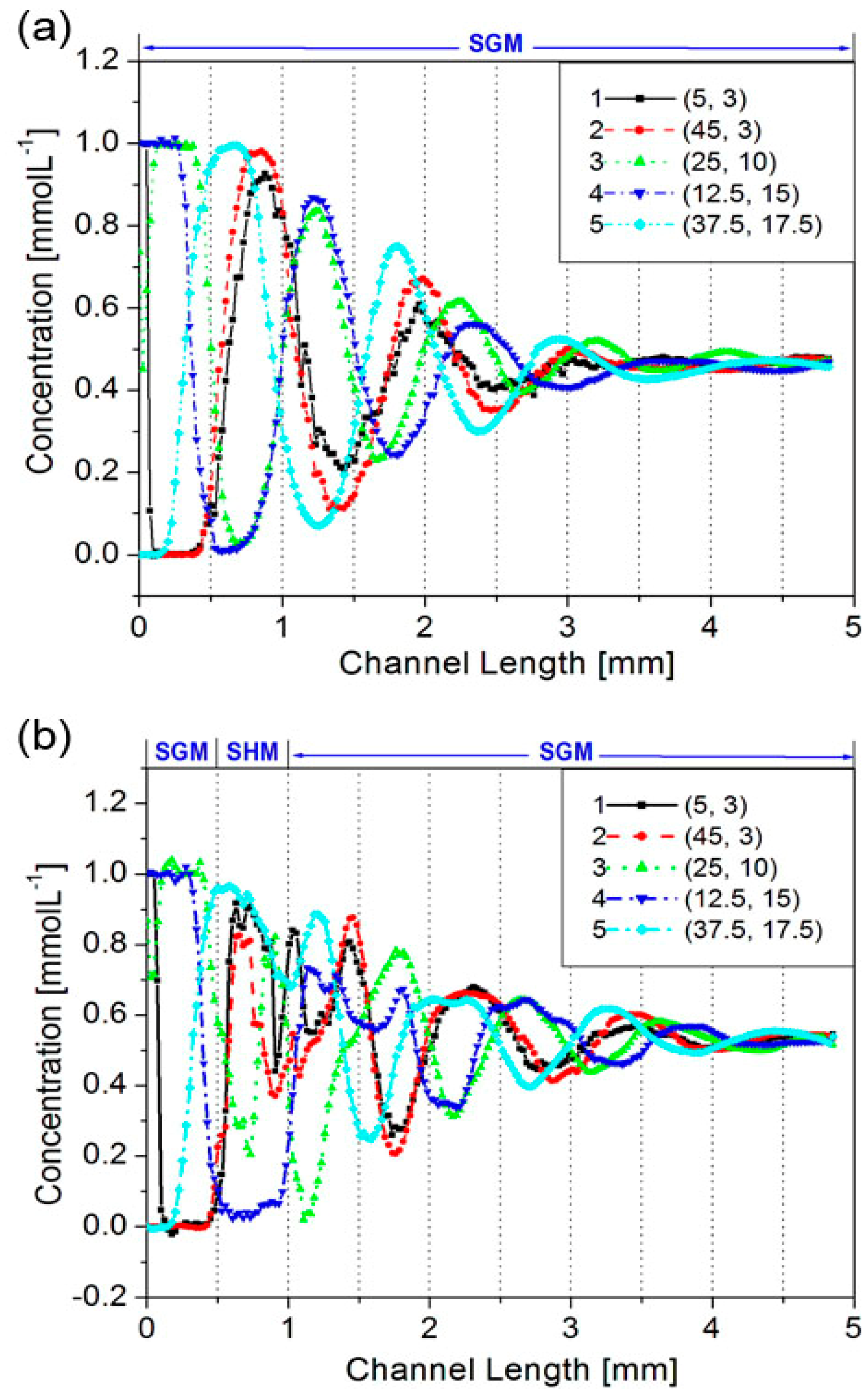
In comparison with the concentration profiles of SGM20, those of SGM20+SHM as shown in
Figure 7(b) appeared to have more chaotic oscillations along the channel length from 0.5 to 1.5 mm. In considering the location of the inserted SHM portion is from 0.5 mm to 1 mm, one should also note that oscillation inertia requires a certain distance along the channel to return to the original fluidic patterns as controlled by the slanted groove. This can be further confirmed by the mixing completion lengths
Lm at different
ε values. As seen from
Table 1, for SGM20+SHM, an
Lm value of 3.4 mm was needed at mixing extent of ε = 0.05, which was larger than 2.6 mm needed in a SGM20 only under same flow conditions. And yet, both of them achieved the mixing extent of ε = 0.01 at almost the same length, with respective
Lm values of 4.6 and 4.7 mm. These results suggested that the mixing within SGM20+SHM did not improve mixing efficiency when a short staggered herringbone grooves segment was inserted into the slanted grooves.
Figure 7.
Concentration profiles for (a) SGM20 and (b) SGM20+SHM. The concentration data were collected along channel length in its flow direction at the fixed cross-section locations represented with [
1] at (5, 3) (unit in μm), [
2] at (45, 3), [
3] at (25, 10), [
4] at (12.5, 15), [
5] at (37.5, 17.5) in the y–z coordinate system of the channel cross section with its bottom-left point set as origin (0, 0). Channel: 20 (h) × 50 (w) μm; groove: 12.5 (w) × 20 (d) μm.
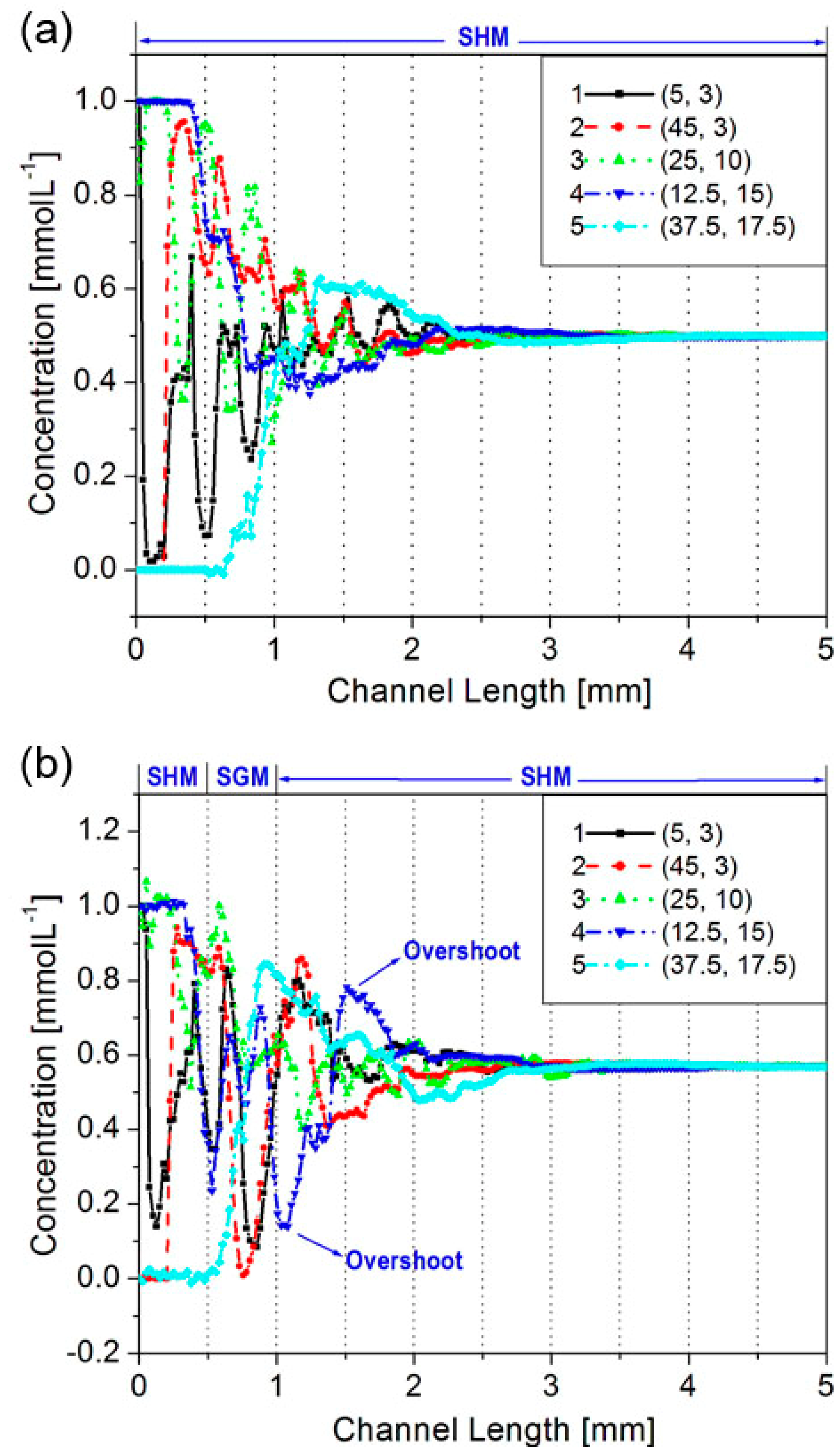
Conversely, we compared the concentration profiles of SHM20 and those of SHM20+SGM, which are shown in
Figure 8. The concentration oscillations in SHM20+SGM became more complex and irregular along the channel length from 0.5 to 1.0 mm. Take Location (12.5, 15) as an example, its concentration oscillated violently along the channel occupied with slanted grooves and then showed two evident overshoots—one downward and one upward—which likely delayed the completion of mixing in the whole channel. Therefore, the resulting
Lm in the SHM20+SGM was greater than that needed in SHM20, as shown in
Table 1. This indicates a less efficient mixing within the SHM20+SGM.
Figure 8.
Concentrations profiles for (a) SHM20 and (b) SHM20+SGM. Other conditions same as in
Figure 7.
Figure 8.
Concentrations profiles for (a) SHM20 and (b) SHM20+SGM. Other conditions same as in
Figure 7.
Furthermore, we calculated the Lm for the other hybrid floor-grooved micromixers with different groove depths or channel heights, and found that all of Lm values in hybrid floor-grooved micromixers were larger than those in the SGM and the SHM. This is probably because the interactions/transitions of the SGM and the SHM interfere the inherent oscillation of flow partners controlled by individual SGM or SHM. As a result, a longer channel length is generally required for the oscillation to return to the original mixing patterns to achieve a complete mixing.
For many micromixing applications, it is important to characterize the mixing length, i.e., Lm. While Lm doesn’t provide detailed information about the mixing process, it is an essential performance parameter. Given that a significant research in the field of lab-on-a-chip is focused on various different applications, such a comprehensive performance parameter is useful for researchers to design specific micromixers. Therefore, the numerical method employed the current has two obvious advantages: (1) to directly reveal the detailed mixing process and (2) to provide a simple guide for a micromixer design in practical applications.
Table 1.
Lm (in mm) for four micromixers at different ε values.
Table 1.
Lm (in mm) for four micromixers at different ε values.
| | ε = 0.05 | ε = 0.01 | ε = 0.005 |
| (1) SGM 20 | 2.6 | 4.7 | —a |
| (2) SGM 20+SHM | 3.4 | 4.6 | —a |
| (3) SHM 20 | 1.8 | 2.8 | 3.3 |
| (4) SHM 20+SGM | 2.1 | 3.1 | 3.7 |


