
Classification for High Resolution Remote Sensing Imagery Using a Fully Convolutional Network


Abstract
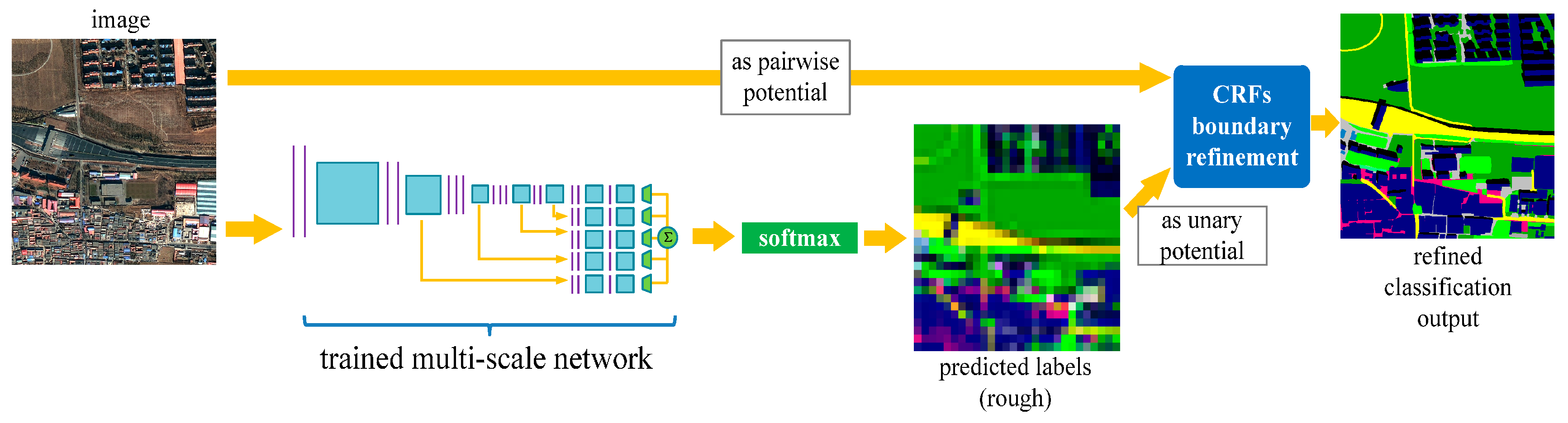
:
1. Introduction
2. Methods
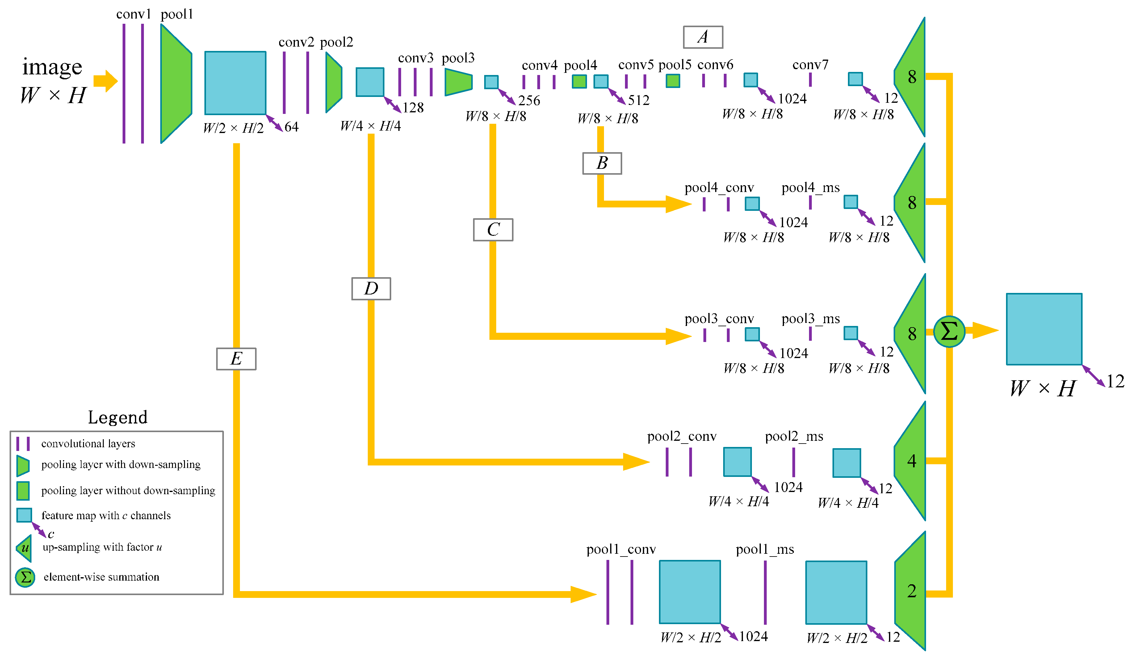
2.1. Network Architecture
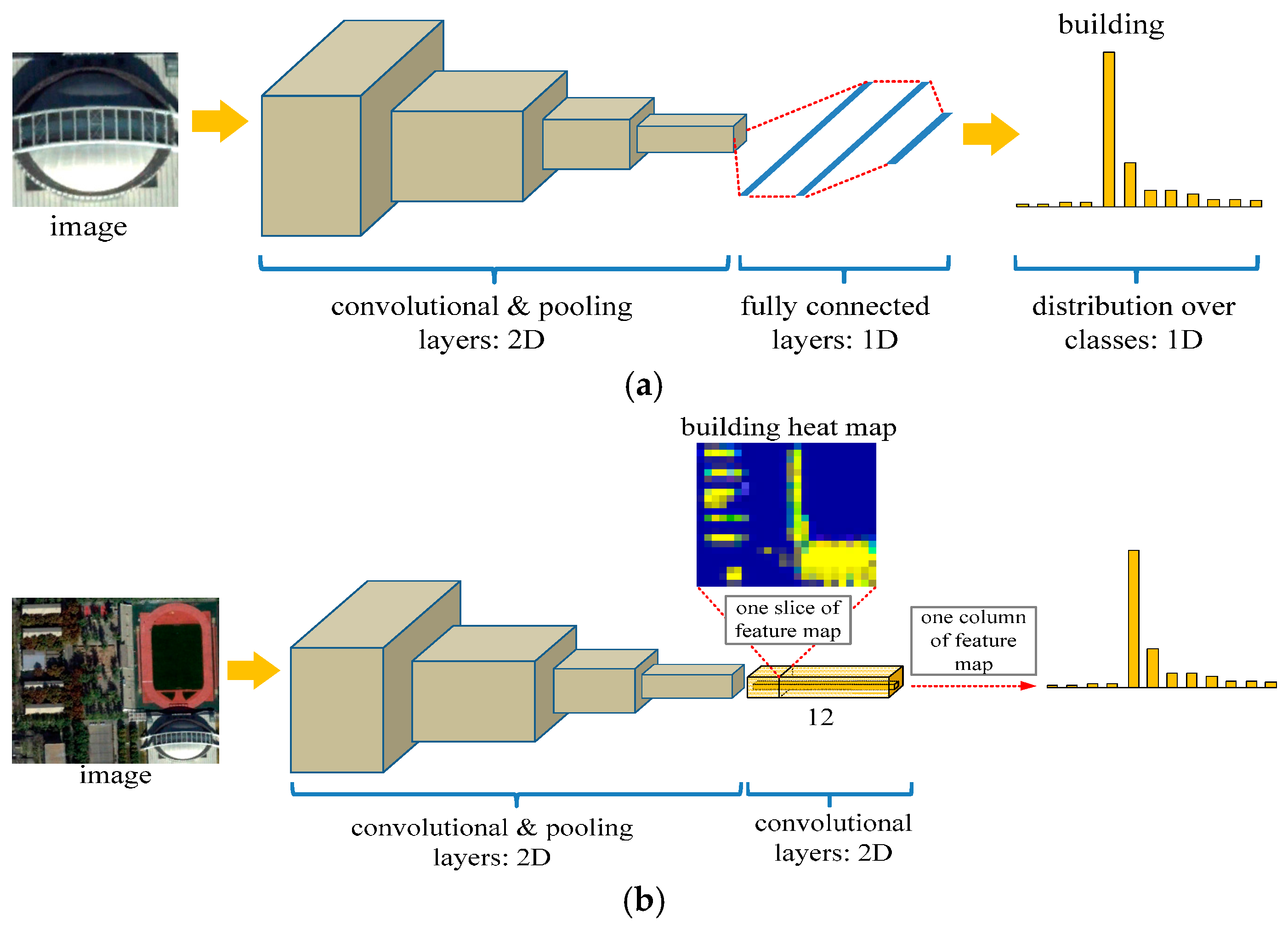
2.1.1. Fully Convolutional Network
- Easy implementation: The FCN architecture is designed brilliantly by replacing the FC layers by convolutional layers, which enables us to take arbitrary sized images as inputs. Additionally, by training entire images at a time instead of patch cropping, FCN does not have to rearrange the output labels together to obtain the label predictions and thus reduces the implementation complexity.
- Higher accuracy: Under the patch-based CNN learning framework, only the “intra-patch” context information is taken into account. Nevertheless, correlations among patches are ignored, which might lead to obvious gaps between patches. Unlike the patch-based CNN, FCN performs the classification in a single-loop manner, and considers the context information overall and seamlessly. Please refer to Section 4.2 for more details.
- Less expensive computation: In patch-based CNN, when using overlapped patches for dense class label generation, such as the study of Martin Lagkvist et al. [28], it introduces too much redundant computations (especially convolutions) on the overlapped regions. By performing a single loop operation, the FCN model makes remarkable progress and allows the large image classification to be implemented in a more effective way.
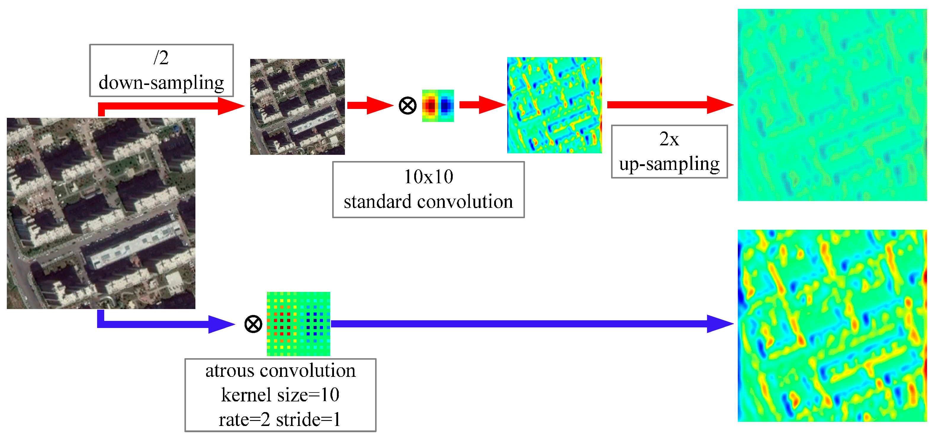
2.1.2. Atrous Convolution for Dense Feature Extraction
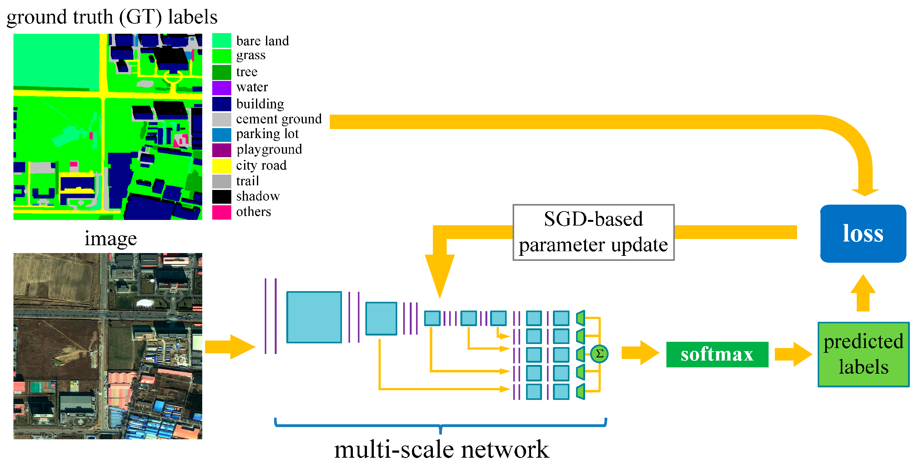
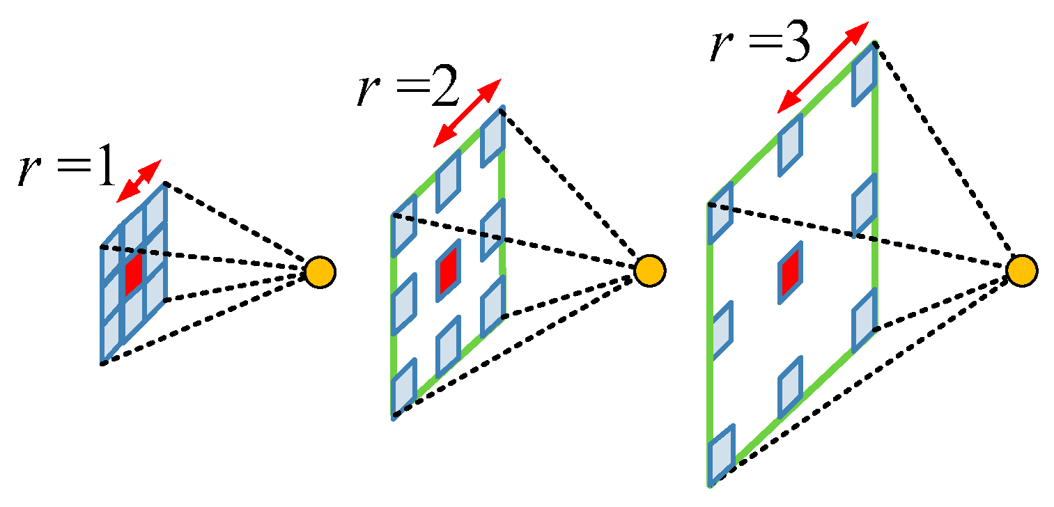
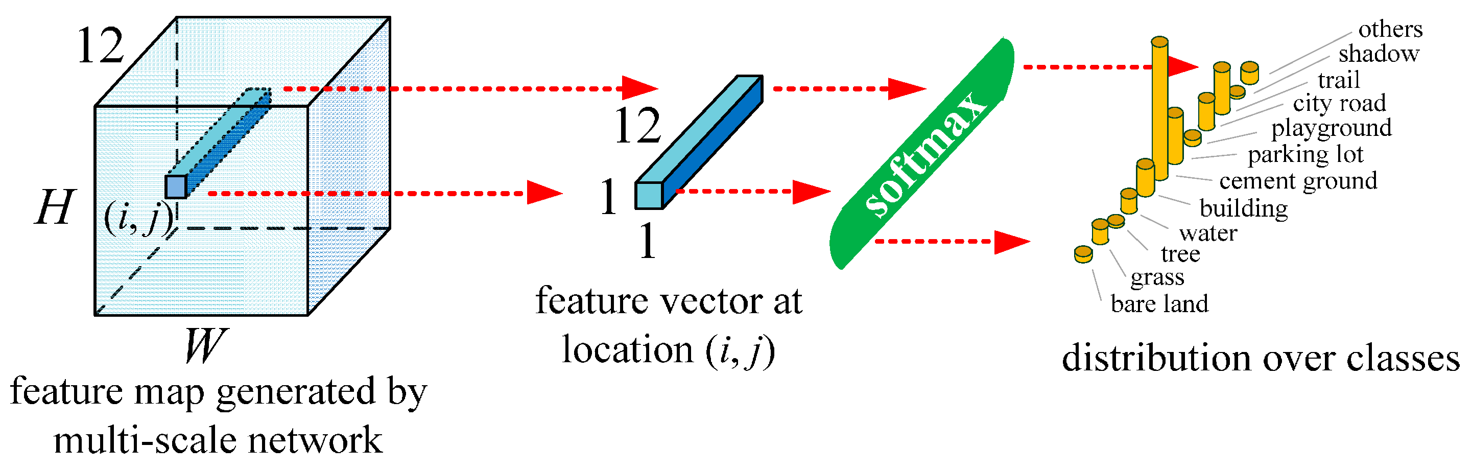
2.1.3. Network Architecture for Multi-Scale Classification
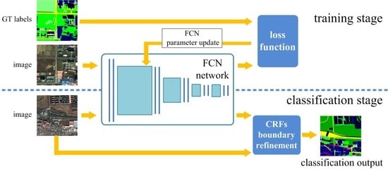
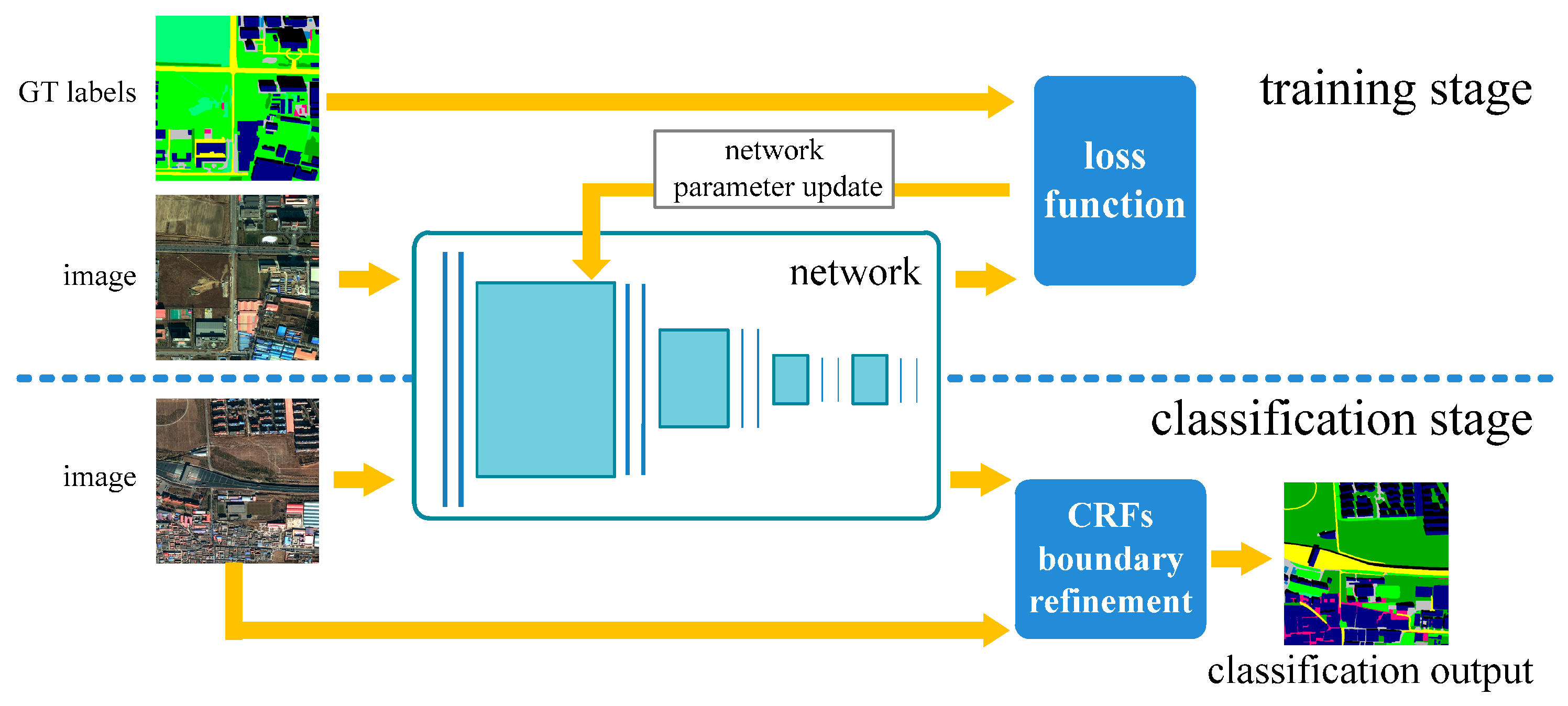
2.2. Network Training
2.3. Classification Using the Trained Network
3. Experiment and Comparison
3.1. Comparison Setup
3.1.1. MR-SVM
- Spectral features: mean, standard deviation, brightness, and max difference for each band.
- Geometric features: area, length, width, length-width ratio, border length, compactness, elliptic fit, rectangular fit, density, shape index, main direction, and symmetry.
- Texture features: Features calculated from the Gray Level Co-occurrence Matrix (GLCM) and the Gray Level Difference Vector (GLDV) with all directions, etc.
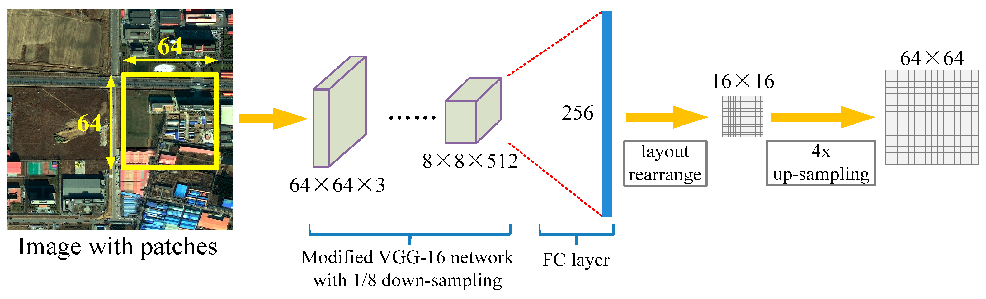
3.1.2. Patch-Based CNN
3.1.3. FCN-8s
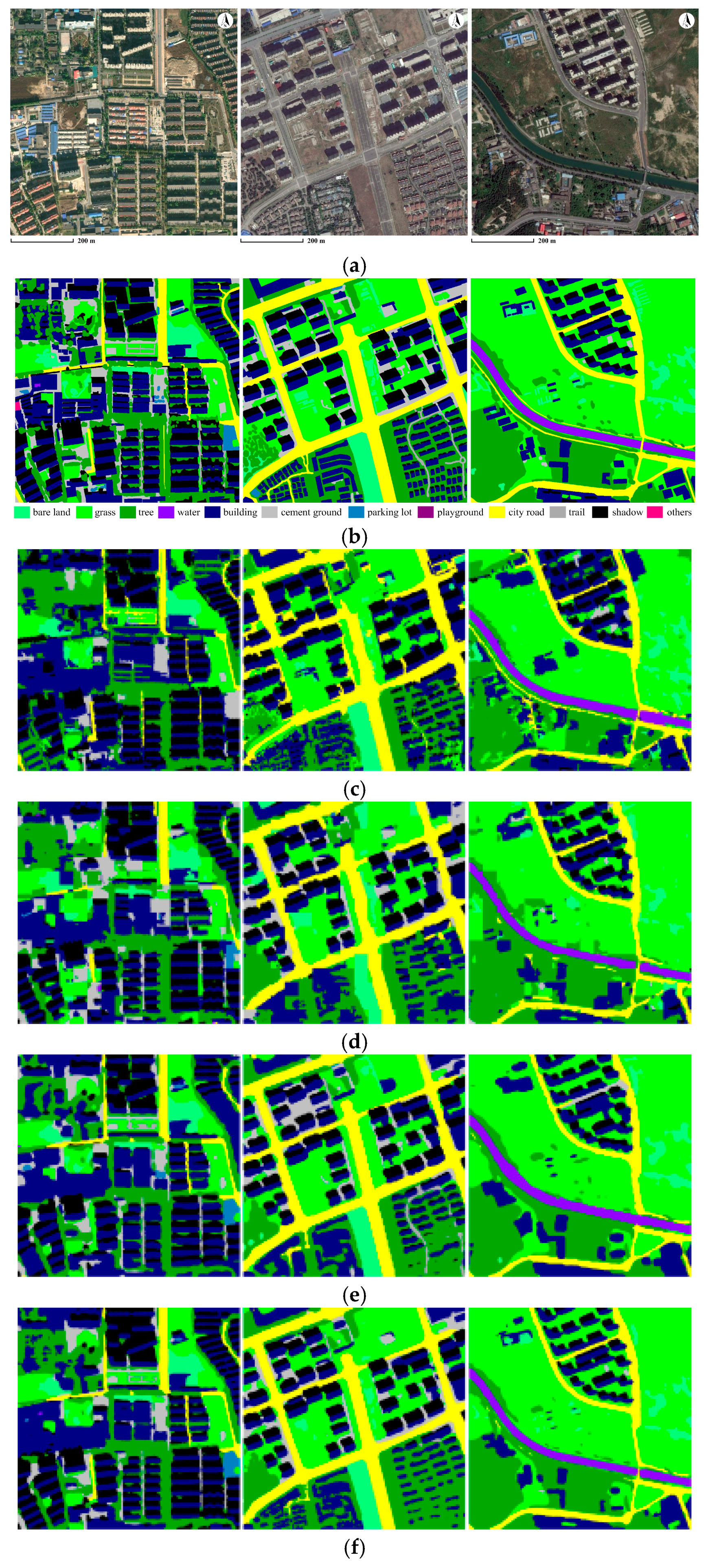
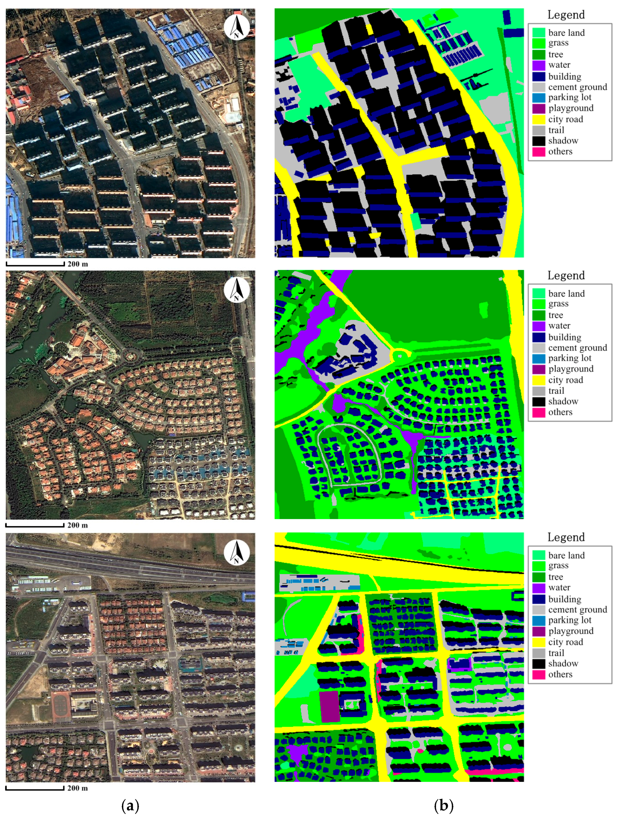
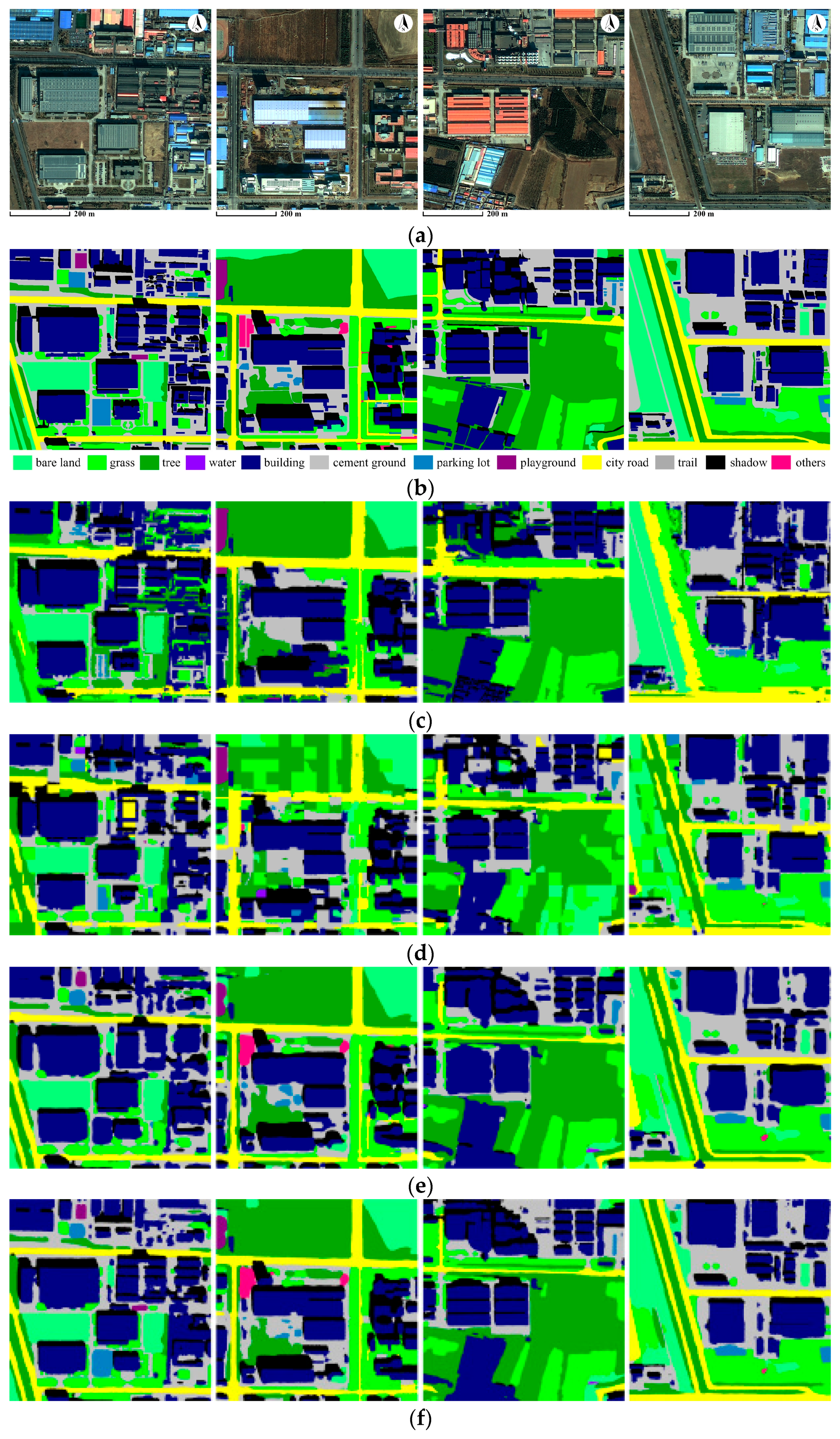
3.2. Experiments and Comparison
4. Discussion
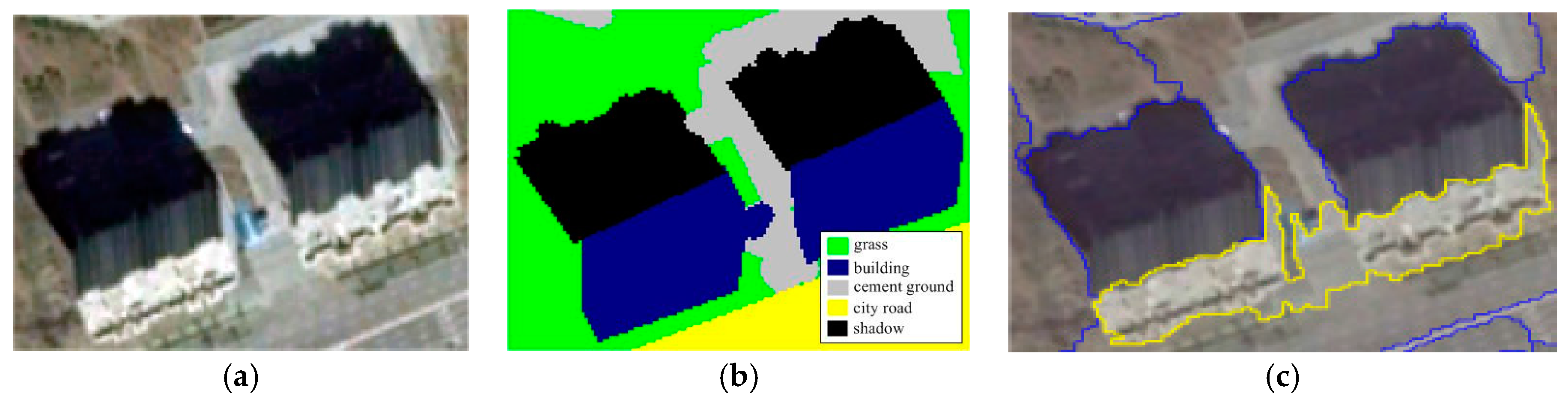
4.1. MR-SVM vs. Our Approach
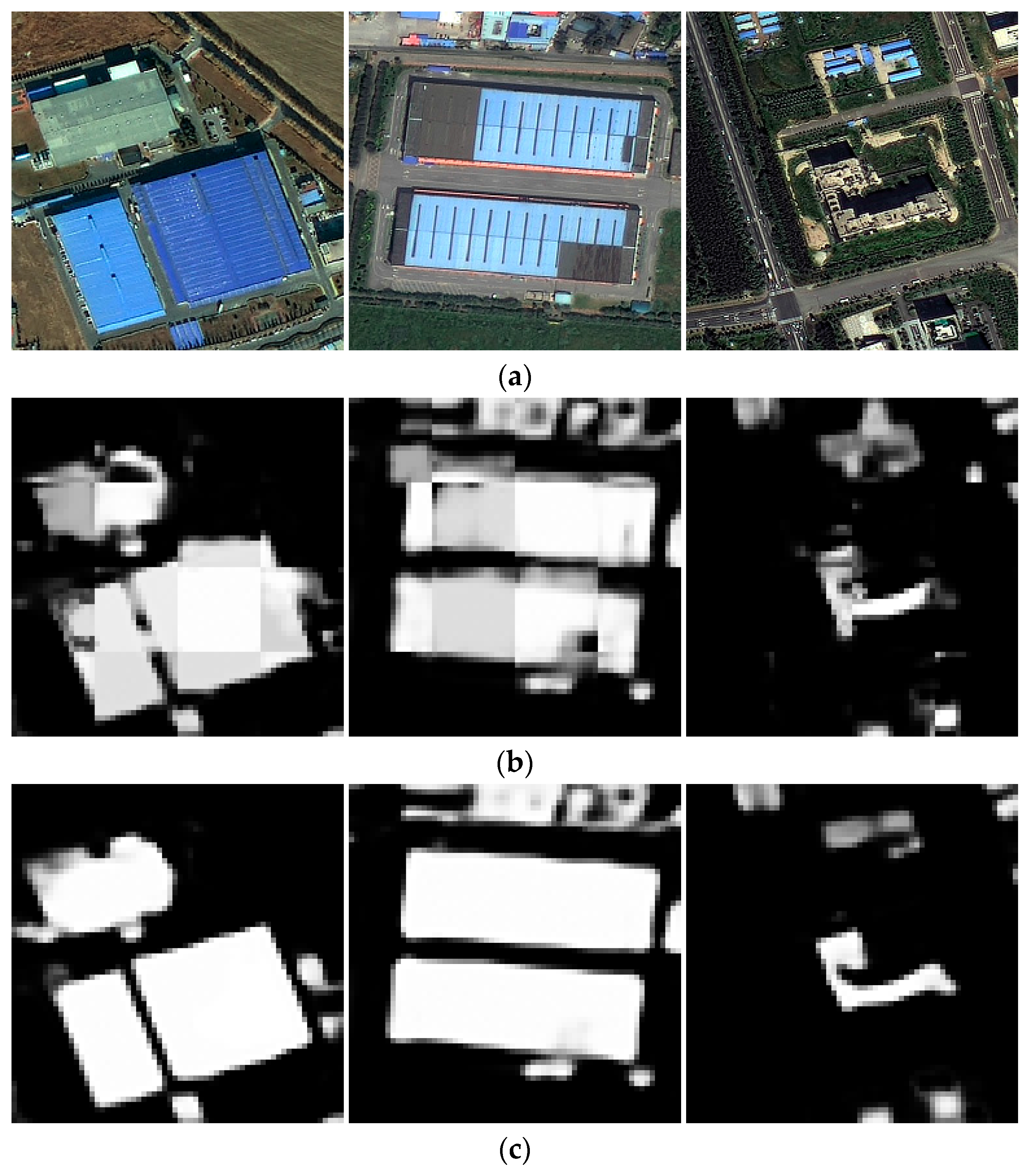
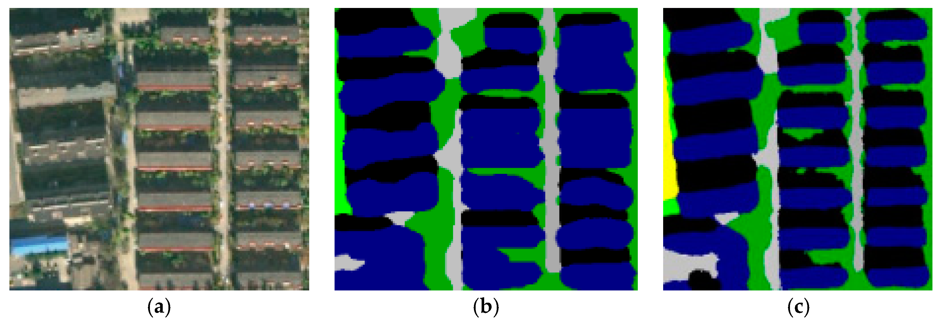
4.2. Patch-Based CNN vs. Our Approach
4.3. FCN-8s vs. Our Approach
5. Conclusions
Acknowledgments
Author Contributions
Conflicts of Interest
References
- MacQueen, J.B. Some Methods for classification and Analysis of Multivariate Observations. Proceedings of 5th Berkeley Symposium on Mathematical Statistics and Probability; University of California Press: Berkeley, CA, USA, 1967; pp. 281–297. [Google Scholar]
- Miller, D.M.; Kaminsky, E.J.; Rana, S. Neural network classification of remote-sensing data. Comput. Geosci. 1995, 21, 377–386. [Google Scholar] [CrossRef]
- Mas, J.; Flores, J. The application of artificial neural networks to the analysis of remotely sensed data. Int. J. Remote Sens. 2008, 29, 617–663. [Google Scholar] [CrossRef]
- Camps-Valls, G.; Bruzzone, L. Kernel-based methods for hyperspectral image classification. IEEE Trans. Geosci. Remote Sens. 2005, 43, 1351–1362. [Google Scholar] [CrossRef]
- Mountrakis, G.; Im, J.; Ogole, C. Support vector machines in remote sensing: A review. ISPRS J. Photogramm. Remote Sens. 2011, 66, 247–259. [Google Scholar] [CrossRef]
- Yuan, Y.; Lin, J.; Wang, Q. Hyperspectral Image Classification via Multitask Joint Sparse Representation and Stepwise MRF Optimization. IEEE Trans. Cybern. 2016, 46, 2966–2977. [Google Scholar] [CrossRef] [PubMed]
- Wang, Q.; Lin, J.; Yuan, Y. Salient Band Selection for Hyperspectral Image Classification via Manifold Ranking. IEEE Trans. Neural Netw. Learn. Syst. 2016, 27, 1279–1289. [Google Scholar] [CrossRef] [PubMed]
- Walter, V. Object-based classification of remote sensing data for change detection. ISPRS J. Photogramm. Remote Sens. 2004, 58, 225–238. [Google Scholar] [CrossRef]
- Definients Image. eCognition User’s Guide 4; Definients Image: Bernhard, Germany, 2004. [Google Scholar]
- Feature Extraction Module Version 4.6. In ENVI Feature Extraction Module User’s Guide; ITT Corporation: Boulder, CO, USA, 2008.
- Baatz, M.; Schäpe, A. Multiresolution Segmentation: An Optimization Approach for High Quality Multi-scale Image Segmentation. In Angewandte Geographische Information Sverarbeitung XII; Herbert Wichmann Verlag: Heidelberg, Germany, 2000; pp. 12–23. [Google Scholar]
- Robinson, D.J.; Redding, N.J.; Crisp, D.J. Implementation of a Fast Algorithm for Segmenting SAR Imagery; DSTO Electronics and Surveillance Research Laboratory: Edinburgh, Australia, 2002. [Google Scholar]
- Cheng, Y. Mean shift, mode seeking, and clustering. IEEE Trans. Pat. 1995, 17, 790–799. [Google Scholar] [CrossRef]
- Fu, G.; Zhao, H.; Li, C.; Shi, L. Segmentation for High-Resolution Optical Remote Sensing Imagery Using Improved Quadtree and Region Adjacency Graph Technique. Remote Sens. 2013, 5, 3259–3279. [Google Scholar] [CrossRef]
- Hinton, G.; Osindero, S.; Welling, M.; Teh, Y.-W. Unsupervised Discovery of Nonlinear Structure Using Contrastive Backpropagation. Science 2006, 30, 725–732. [Google Scholar] [CrossRef] [PubMed]
- Deep Learning. Available online: https://en.wikipedia.org/wiki/Deep_learning (accessed on 3 May 2017).
- Hinton, G.E.; Osindero, S.; Teh, Y.W. A Fast Learning Algorithm for Deep Belief Nets. Neural Comput. 2006, 18, 1527–1554. [Google Scholar] [CrossRef] [PubMed]
- Convolutional Neural Networks (LeNet)—DeepLearning 0.1 Documentation. DeepLearning 0.1. LISA Lab. Retrieved 31 August 2013. Available online: http://deeplearning.net/tutorial/lenet.html (accessed on 5 May 2017).
- Graves, A.; Liwicki, M.; Fernandez, S.; Bertolami, R.; Bunke, H.; Schmidhuber, J. A Novel Connectionist System for Improved Unconstrained Handwriting Recognition. IEEE Trans. Pattern Anal. Mach. Intell. 2009, 31, 855–868. [Google Scholar] [CrossRef] [PubMed]
- Krizhevsky, A.; Sutskever, I.; Hinton, G.E. Imagenet classification with deep convolutional neural networks. In Proceedings of the Neural Information Processing Systems (NIPS) Conference, La Jolla, CA, USA, 3–8 December 2012. [Google Scholar]
- Ciresan, D.; Meier, U.; Schmidhuber, J. Multi-column deep neural networks for image classification. In Proceedings of the Conference on Computer Vision and Pattern Recognition (CVPR), Providence, RI, USA, 16–21 June 2012; pp. 3642–3649. [Google Scholar]
- Nguyen, T.; Han, J.; Park, D.C. Satellite image classification using convolutional learning. In Proceedings of the AIP Conference, Albuquerque, NM, USA, 7–10 October 2013; pp. 2237–2240. [Google Scholar]
- Wang, J.; Song, J.; Chen, M.; Yang, Z. Road network extraction: A neural-dynamic framework based on deep learning and a finite state machine. Int. J. Remote Sens. 2015, 36, 3144–3169. [Google Scholar] [CrossRef]
- Castelluccio, M.; Poggi, G.; Sansone, C.; Verdoliva, L. Land Use Classification in Remote Sensing Images by Convolutional Neural Networks. arXiv 2015. [Google Scholar]
- Hu, F.; Xia, G.S.; Hu, J.; Zhang, L. Transferring deep convolutional neural networks for the scene classification of high-resolution remote sensing imagery. Remote Sens. 2015, 7, 14680–14707. [Google Scholar] [CrossRef]
- Zhou, W.; Newsam, S.; Li, C.; Shao, Z. Learning Low Dimensional Convolutional Neural Networks for High-Resolution Remote Sensing Image Retrieval. arXiv 2016. [Google Scholar]
- Mnih, V. Machine Learning for Aerial Image Labeling. Ph.D. Thesis, University of Toronto, Toronto, ON, Canada, 2013. [Google Scholar]
- Lagkvist, M.; Kiselev, A.; Alirezaie, M.; Loutfi, A. Classification and Segmentation of Satellite Orthoimagery Using Convolutional Neural Networks. Remote Sens. 2016, 8, 329. [Google Scholar] [CrossRef]
- Long, J.; Shelhamer, E.; Darrell, T. Fully Convolutional Networks for Semantic Segmentation. In Proceedings of the Conference on Computer Vision and Pattern Recognition (CVPR), Boston, MA, USA, 7–12 June 2015. [Google Scholar]
- Chen, L.C.; Kokkinos, I.; Murphy, K.; Yuille, A.L. Semantic Image Segmentation with Deep Convolutional Nets and Fully Connected CRFs. In Proceedings of the International Conference on Learning Representations (ICLR), San Diego, CA, USA, 7–9 May 2015. [Google Scholar]
- Paisitkriangkrai, S.; Sherrah, J.; Janney, P.; Van den Hengel, A. Effective Semantic Pixel labelling with Convolutional Networks and Conditional Random Fields. In Proceedings of the Conference on Computer Vision and Pattern Recognition (CVPR), Boston, MA, USA, 7–12 June 2015. [Google Scholar]
- Zheng, S.; Jayasumana, S.; Romera-Paredes, B.; Vineety, V.; Su, Z. Conditional Random Fields as Recurrent Neural Networks. In Proceedings of the Conference on Computer Vision and Pattern Recognition (CVPR), Las Vegas, NV, USA, 26 June–1 July 2016. [Google Scholar]
- Sherrah, J. Fully Convolutional Networks for Dense Semantic Labelling of High-Resolution Aerial Imagery. arXiv 2016. [Google Scholar]
- Marmanis, D.; Wegner, J.D.; Galliani, S.; Schindler, K.; Datcu, M.; Stilla, U. Semantic segmentation of aerial images with an ensemble of CNSS. In Proceedings of the ISPRS Annals of the Photogrammetry, Remote Sensing and Spatial Information Sciences, Prague, Czech Republic, 12–19 July 2016. [Google Scholar]
- Maggiori, E.; Tarabalka, Y.; Charpiat, G.; Alliez, P. Fully Convolutional Neural Networks for Remote Sensing Image Classification. In Proceedings of the 2016 IEEE International Geoscience and Remote Sensing Symposium (IGARSS), Beijing, China, 10–15 July 2016; pp. 5071–5074. [Google Scholar]
- Maggiori, E.; Tarabalka, Y.; Charpiat, G.; Alliez, P. Convolutional Neural Networks for Large-Scale Remote Sensing Image Classification. IEEE Trans. Geosci. Remote Sens. 2017, 2, 645–657. [Google Scholar] [CrossRef]
- Maggiori, E.; Tarabalka, Y.; Charpiat, G.; Alliez, P. High-Resolution Semantic Labeling with Convolutional Neural Networks. arXiv 2016. [Google Scholar]
- Simonyan, K.; Zisserman, A. Very deep convolutional networks for large-scale image recognition. arXiv 2014. [Google Scholar]
- He, K.; Zhang, X.; Ren, S.; Sun, J. Deep residual learning for image recognition. arXiv 2015. [Google Scholar]
- Szegedy, C.; Ioffe, S.; Vanhoucke, V.; Alemi, A. Inception-v4, Inception-ResNet and the Impact of Residual Connections on Learning. arXiv 2016. [Google Scholar]
- Bertasius, G.; Shi, J.; Torresani, L. Deepedge: A multiscale bifurcated deep network for top-down contour detection. In Proceedings of the Conference on Computer Vision and Pattern Recognition (CVPR), Boston, MA, USA, 7–12 June 2015. [Google Scholar]
- Xie, S.; Tu, Z. Holistically-Nested Edge Detection. arXiv 2015. [Google Scholar]
- Krahenbuhl, P.; Koltun, V. Efficient Inference in Fully Connected CRFs with Gaussian Edge Potentials. In Proceedings of the 24th International Conference on Neural Information Processing Systems (NIPS), Granada, Spain, 12–15 December 2011. [Google Scholar]
- Nussbaum, S.; Niemeyer, I.; Canty, M.J. SEATH—A new tool for automated feature extraction in the context of object-based image analysis. In Proceedings of the 1st International Conference on Object-Based Image Analysis, Salzburg, Austria, 4–5 July 2006. XXXVI-4/C42. [Google Scholar]
- Chang, C.C.; Lin, C.J. LIBSVM: A library for support vector machines. ACM Trans. Intell. Syst. Technol. 2011, 2. [Google Scholar] [CrossRef]


| Experiment | Scale | Shape | Compact |
|---|---|---|---|
| Exp.A-(1) | 115 | 0.5 | 0.5 |
| Exp.A-(2) | 140 | 0.3 | 0.8 |
| Exp.A-(3) | 105 | 0.4 | 0.5 |
| Exp.A-(4) | 100 | 0.4 | 0.7 |
| Exp.B-(1) | 120 | 0.3 | 0.5 |
| Exp.B-(2) | 80 | 0.5 | 0.4 |
| Exp.B-(3) | 85 | 0.5 | 0.7 |
| Approach | Index | Exp.A-(1) | Exp.A-(2) | Exp.A-(3) | Exp.A-(4) | Exp.B-(1) | Exp.B-(2) | Exp.B-(3) | Mean |
|---|---|---|---|---|---|---|---|---|---|
| MR-SVM | Precision | 0.67 | 0.72 | 0.67 | 0.66 | 0.65 | 0.73 | 0.64 | 0.68 |
| Recall | 0.52 | 0.59 | 0.52 | 0.63 | 0.39 | 0.51 | 0.74 | 0.56 | |
| Kappa | 0.55 | 0.66 | 0.62 | 0.65 | 0.54 | 0.64 | 0.64 | 0.61 | |
| Patch-based CNN | Precision | 0.68 | 0.64 | 0.71 | 0.55 | 0.73 | 0.76 | 0.70 | 0.68 |
| Recall | 0.61 | 0.61 | 0.70 | 0.73 | 0.47 | 0.58 | 0.74 | 0.63 | |
| Kappa | 0.64 | 0.69 | 0.62 | 0.70 | 0.63 | 0.71 | 0.75 | 0.68 | |
| FCN-8s | Precision | 0.83 | 0.84 | 0.68 | 0.66 | 0.81 | 0.78 | 0.83 | 0.78 |
| Recall | 0.71 | 0.79 | 0.80 | 0.80 | 0.66 | 0.66 | 0.79 | 0.74 | |
| Kappa | 0.73 | 0.80 | 0.81 | 0.80 | 0.76 | 0.81 | 0.82 | 0.79 | |
| Ours | Precision | 0.86 | 0.87 | 0.74 | 0.68 | 0.84 | 0.78 | 0.92 | 0.81 |
| Recall | 0.83 | 0.78 | 0.81 | 0.82 | 0.70 | 0.68 | 0.84 | 0.78 | |
| Kappa | 0.79 | 0.85 | 0.84 | 0.83 | 0.78 | 0.84 | 0.89 | 0.83 |
| Experiment | GT/Predicted Class | Building | Cement Ground | City Road |
|---|---|---|---|---|
| Exp.A-(1) | Building | 0.91 | 0.05 | 0.02 |
| Cement ground | 0.13 | 0.76 | 0.02 | |
| City road | 0.02 | 0.01 | 0.95 | |
| Exp.A-(2) | Building | 0.92 | 0.03 | 0.03 |
| Cement ground | 0.05 | 0.79 | 0.06 | |
| City Road | 0.01 | 0.04 | 0.89 | |
| Exp.A-(3) | Building | 0.91 | 0.02 | 0.05 |
| Cement ground | 0.10 | 0.82 | 0.03 | |
| City road | 0.05 | 0.04 | 0.82 | |
| Exp.A-(4) | Building | 0.95 | 0.03 | 0.00 |
| Cement ground | 0.07 | 0.81 | 0.05 | |
| City road | 0.01 | 0.01 | 0.93 | |
| Exp.B-(1) | Building | 0.90 | 0.02 | 0.01 |
| Cement ground | 0.26 | 0.65 | 0.01 | |
| City road | 0.11 | 0.03 | 0.84 | |
| Exp.B-(2) | Building | 0.83 | 0.01 | 0.00 |
| Cement ground | 0.08 | 0.75 | 0.15 | |
| City road | 0.01 | 0.01 | 0.96 | |
| Exp.B-(3) | Building | 0.87 | 0.06 | 0.01 |
| Cement ground | 0.03 | 0.70 | 0.04 | |
| City road | 0.10 | 0.01 | 0.87 |
© 2017 by the authors. Licensee MDPI, Basel, Switzerland. This article is an open access article distributed under the terms and conditions of the Creative Commons Attribution (CC BY) license (http://creativecommons.org/licenses/by/4.0/).
Share and Cite
Fu, G.; Liu, C.; Zhou, R.; Sun, T.; Zhang, Q. Classification for High Resolution Remote Sensing Imagery Using a Fully Convolutional Network. Remote Sens. 2017, 9, 498. https://doi.org/10.3390/rs9050498
Fu G, Liu C, Zhou R, Sun T, Zhang Q. Classification for High Resolution Remote Sensing Imagery Using a Fully Convolutional Network. Remote Sensing. 2017; 9(5):498. https://doi.org/10.3390/rs9050498
Chicago/Turabian StyleFu, Gang, Changjun Liu, Rong Zhou, Tao Sun, and Qijian Zhang. 2017. "Classification for High Resolution Remote Sensing Imagery Using a Fully Convolutional Network" Remote Sensing 9, no. 5: 498. https://doi.org/10.3390/rs9050498
APA StyleFu, G., Liu, C., Zhou, R., Sun, T., & Zhang, Q. (2017). Classification for High Resolution Remote Sensing Imagery Using a Fully Convolutional Network. Remote Sensing, 9(5), 498. https://doi.org/10.3390/rs9050498