Article

Cost-Effective Class-Imbalance Aware CNN for Vehicle Localization and Categorization in High Resolution Aerial Images

1
Institute of Automation Chinese Academy of Sciences, Beijing 100190, China
2
University of Chinese Academy of Science, Beijing 100049, China
*
Authors to whom correspondence should be addressed.
Remote Sens. 2017, 9(5), 494; https://doi.org/10.3390/rs9050494
Submission received: 26 February 2017 / Revised: 28 April 2017 / Accepted: 15 May 2017 / Published: 18 May 2017
(This article belongs to the Special Issue Learning to Understand Remote Sensing Images)

Abstract

:
Joint vehicle localization and categorization in high resolution aerial images can provide useful information for applications such as traffic flow structure analysis. To maintain sufficient features to recognize small-scaled vehicles, a regions with convolutional neural network features (R-CNN) -like detection structure is employed. In this setting, cascaded localization error can be averted by equally treating the negatives and differently typed positives as a multi-class classification task, but the problem of class-imbalance remains. To address this issue, a cost-effective network extension scheme is proposed. In it, the correlated convolution and connection costs during extension are reduced by feature map selection and bi-partite main-side network construction, which are realized with the assistance of a novel feature map class-importance measurement and a new class-imbalance sensitive main-side loss function. By using an image classification dataset established from a set of traditional real-colored aerial images with 0.13 m ground sampling distance which are taken from the height of 1000 m by an imaging system composed of non-metric cameras, the effectiveness of the proposed network extension is verified by comparing with its similarly shaped strong counter-parts. Experiments show an equivalent or better performance, while requiring the least parameter and memory overheads are required.

Graphical Abstract

1. Introduction

For most of the sliding window-based vehicle detection methods involving localization and categorization, predictions are often performed in a separated manner, where the categories are estimated after the positional information is obtained. In the localization process—also called vehicle detection in its narrow sense—the positional existence of vehicles is estimated by analyzing the features extracted from the sliding window that moves across the region of interest with a pre-defined route and stepping pattern. The features used for vehicle detection can either be hand-crafted shallow descriptors or the deep features generated by convolutional neural network (CNN). Shallow features such as Haar [1], histogram of oriented gradients (HOG) [2,3], and local binary pattern (LBP) [3], etc.—although they are less robust and accurate as the deep ones—can make a good compromise between speed and efficiency when the computational resources or the quantity of training samples are very limited. However, once these limitations no longer exist, the detection methods based on deep features are often superior with strong resistance to disturbances in scale, lighting condition, and shadow, and their supreme performances have been repeatedly verified in many studies [4,5,6,7,8]. For these CNN-based methods, their underlying structures generally follow the regions with convolutional neural network features (R-CNN)  [9] or its accelerated variants [10,11,12,13] with region of interest (ROI)-pooling [14]. More specifically, the R-CNN detector—whose features are calculated from the full-scale input image without sub-sampling—despite being primitive, turns out to be informative for recognizing small objects. Because of this, in large aerial images with small-scaled vehicles, R-CNN-like structure [5,6,7,8] is often preferred over those with ROI-pooling [4,15], which is also used in this article. Moreover, it can be accelerated by lossless preprocessing means such as saliency detection [16,17] and objectness filtering [8].
Once the vehicle locations are obtained, they are fed to the subsequent categorization process as positional indications to extract features. Similar to the localization process, features for classification can be produced by either shallow or deep models. At present, limited by the number of publicly available high-resolution aerial image datasets, only a small number of vehicle detection methods involve a classification procedure [18,19,20]. Among these limited publications, authors in both [19] and [20] tried to categorize vehicles by the “SVM + feature” strategy, while in [20] the strong influence of the class-imbalance issue on  classification accuracies has been observed.
The separated estimation scheme discussed above is quite natural, and has been adopted for the positional classification of many general objects [10,12,13,21]. However, it could be troublesome for classifying targets as small as vehicles. Considering a private car only six pixels in width, any location error greater than four pixels will miss the main body of the vehicle and make the following categorization meaningless. Detecting objects in dense scenes can be untangled via density estimation [22] or object counting [23], which has already been validated for congested traffic scene classification [24]. While in this article, without loss of generality, taking the R-CNN detector as a common CNN-based classifier as in [7,8], the previously mentioned cascaded localization error can be avoided by treating the samples with deviation as a negative class and classifying them alongside the accurately centered but differently typed positives.
This arrangement primarily solves the problems caused by the small target scale, and strictly constrains type classification to those accurately located situations. Except for that, however, the introduction of a large quantity of negatives further skews the unbalanced categorical distributions between vehicle types. To address this problem, a bi-partite network extension driven by a class-imbalance-aware cost function is proposed. This cost function is designed based on the idea of providing the two network components with different training losses, intentionally correlating the extended component to the minority classes which are badly classified. Moreover, to reduce the extension costs, the extended components are built with feature maps from lower convolutional layers selected by a novel importance measurement. Notably, compared with other similarly-shaped structures, this proposed modification scheme is capable of achieving equal or better performance with much less extension overhead.
The rest of the paper is arranged as follows: Related and similar works are discussed in Section 2. The CNN basics and the semantic interpretation of convolutional kernels are given in Section 3. The proposed extension and its details are introduced in Section 4. Dataset preparation, experiment setup, and analysis of experimental results are presented in Section 5. Conclusive discussions on the experiments are given in Section 6. Section 7 concludes the paper.

2. Related Work

Class imbalance is a ubiquitous issue existing in nearly every real-life classification problem. As it has been intensively studied for more than two decades, many comprehensive and insightful reviews have been published to generalize the methods on this topic [25,26,27,28]. According to [28], these proposed treatments generally fall within three categories: data-level, algorithm-level, and hybrid treatments. The data-level methods focus on balancing the training samples, modifying their distributions via over-sampling or under-sampling. Typical techniques would include synthetic minority over-sampling technique (SMOTE) [29] and many of its variants, such as adaptive synthetic sampling (ADASYN) [30] and cluster-based oversampling (CBO) [31]. The algorithm-level methods—which are mostly based on the cost-sensitive principle [32,33]—alleviate the bias with majority classes by assigning greater penalties for the minority ones in training. The hybrid methods (e.g., the ensemble style classifiers [34]) take the advantages of the previous two for further performance enhancement, which is common, as mentioned in [25,28].
All of the previously mentioned means are for “shallow” models, but their class-imbalance-addressing principles still apply to the deep learning-based classifiers [35]. For instance, the re-sampling tricks work fine [36,37], although some more advanced dealing methods (e.g., the generative adversarial network (GAN) [38]) should be used to avoid noise and over-fitting in the re-sampling. Similarly, algorithm-level cost function reformation is also widely applicable [39,40,41], where the softmax loss [42,43], cross-entropy loss [39], and logistic regression [44] are mostly taken as the basis format. More recently, a new branch of cost-sensitive methods based on improving the underlying micro feature space structure have appeared, and they have achieved a significant improvement by constraining the relative sample distances [35,45,46,47]. Representative methods in this category include the triplet loss [43,45], quintuplet loss [35], and the center loss [47], which are now hotly debated in the academy.
Although the proposed method in this article generally follows the algorithm-level principle, it is more concerned about achieving a robust performance improvement with less or no influence on the original structure. This goal is achieved by re-balancing the classification bias with the assistance of an extra network component, where the structural expansion cost is kept at a minimum by the incorporative usage of feature map selection.
Plain extension of the convolutional kernel was theoretically analyzed in [48] without involving the class-imbalance issue. Structural extension is a common method for network performance enhancement whose underlying intentions focus either on feature space enhancement [41,48,49,50] or strong prior generation [51,52], and it has been applied to numerous topics, including classification [49,51], tracking [52], edge detection [41], etc. Specifically, only one paper [53] has been found to directly address the class-imbalance issue by combining the feature vectors outputted from a dual arrangement of auto-encoders, where the issue of cost-efficiency has not been emphasized.
Feature map selection can be viewed as a special case of feature selection based on the CNN structure. Consistent with the feature selection methods, it also has two categories with three types [54]: the first category includes the filters [55,56,57], where ranks of the features are obtained without the help of classifiers; the second category employs the predictor, and for the included types, wrappers [58] explicitly score the feature, while the embedded methods [59,60,61] do it implicitly in the training process. Mostly, feature map selection is used for the enhancement of network performance. However, for the purpose of structural simplification, the wrappers principle would be more appropriate in our case.
Due to such specialized requirement, per the brief review above, few studies have tried to make a combinatorial usage of these two methods to seek effective network performance improvement with optimized expansion costs. So, the method proposed in this article acts as a novel approach to  the class-imbalance problem with convenient usage, where no tricky hard negative mining or parameter selection is involved.

3. Background

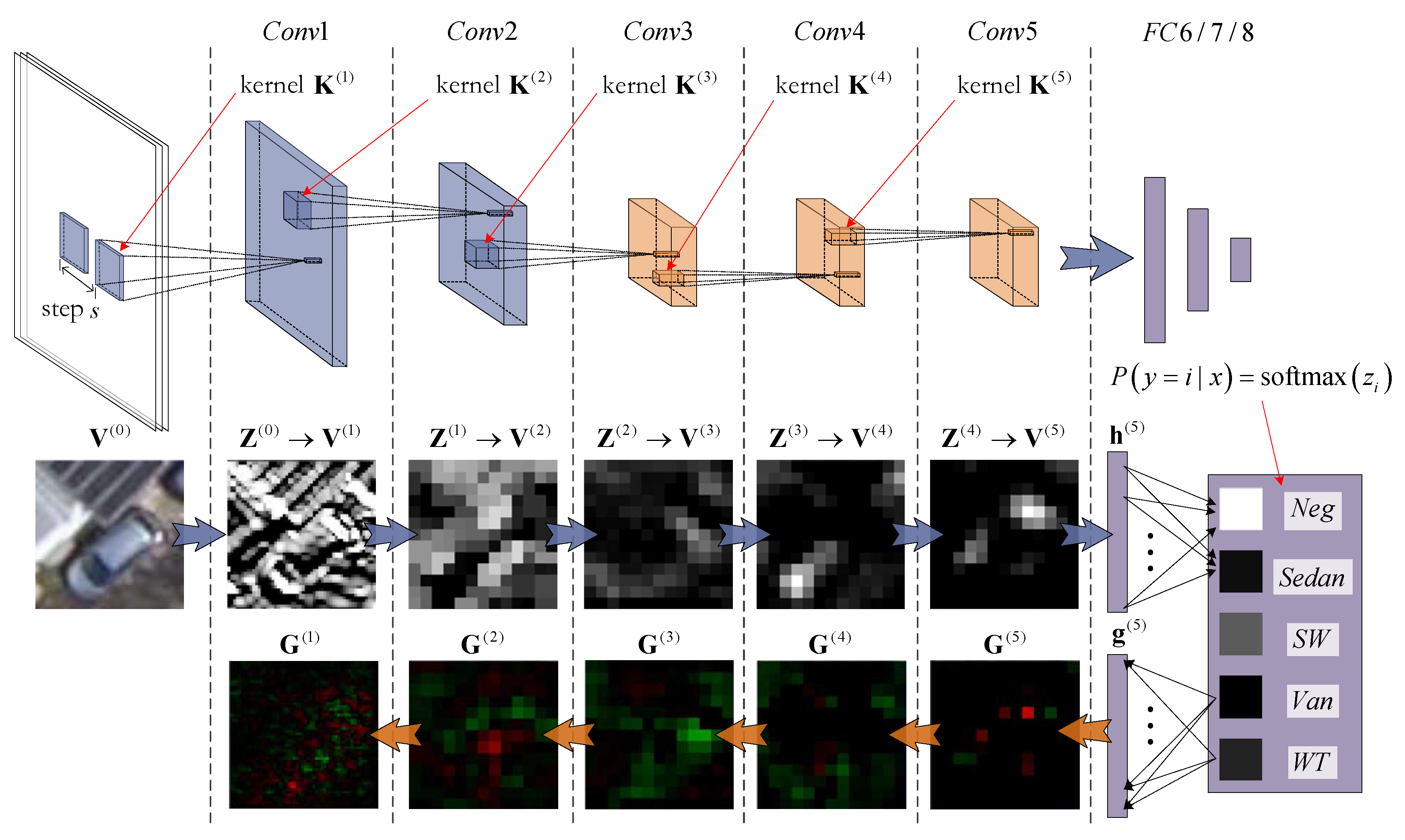
3.1. Basic Knowledge of Convolutional Neural Networks

Convolutional neural networks (CNNs) currently dominate computer vision studies, with constant state-of-the-art performance in almost every topic to which they are applied. CNNs are a special kind of deep belief network (DBN) with components called convolutional layers, composed of units called kernels or filters. Due to space limitations,  a very brief introduction based on [62] is given for the principles of DBN and CNN and to help with the clarity of symbols. Firstly, a normal DBN can be viewed as a stack of fully-connected layers, where each layer has a set of learnt parameters θ composed of connection weights W and bias b . During the forward propagation, every input vector x will be processed by an affine transformation to get the output z , as in Equation (1).
z = W T x + b
In practice, the output z will be further corrected by a nonlinear function such as h = g z to overcome the XOR problem, where the rectified linear unit (or ReLU) [63,64] will always be chosen as the g · . At the final stage of forward propagation, an output vector from the topmost fully-connected layer would be transformed by a probability distribution function (e.g., the softmax function) before being outputted. The softmax function defined in Equation (2) is one of the most commonly used Bernoulli distribution outputs calculated through normalized exponential transformation.
P y = i | x = softmax z i = exp z i j exp z j
To obtain the highest probability on the correct class label y on the input x , this output for softmax function is minimized by its negative log-likelihood format, which is defined in Equation (3).
J θ ; x , y = L y ^ , y + λ · Ω θ L y ^ , y = log softmax z i = log j exp z j z i
Here, J · is the loss to be minimized during training, and L y ^ , y is the softmax-based loss term in which y and y ^ are the true and estimated labels for input x . Ω · is some regularization term with restrictions defined on the network parameters θ (e.g., the weights W or biases b ). More often than not, gradient descent-based optimization is employed to reduce the value of J · , where the updating gradient from the softmax loss is g = y ^ J , based on the estimated label. Similarly, the updating gradients for W and b are defined in Equation (4), calculated by the chain rule.
W ( k ) J = h ( k 1 ) T g , b ( k ) J = g
W ( k ) W ( k ) + α · W ( k ) J , b ( k ) b ( k ) + α · b ( k ) J
W ( k ) and b ( k ) are the weights and bias for the fully connected layer at level k, whose rectified output is denoted as h ( k 1 ) . During the back propagation, at each layer, the weights and bias are updated by adding the deviations W ( k ) J and b ( k ) J , with the latter ones multiplied by a learning rate α to control the convergence rate, as in Equation (5).
Those are the cases for the DBN, while all things are almost identical in the case of CNN, except for the part involving the convolutional layers. Convolutional layers can be treated as a special kind of fully-connected layer with shared connection weights held by kernels. Take the network in Figure 1 for illustration; considering a 4-D kernel tensor K ( k ) from the kth convolutional layer, during the back propagation, the input signal data V ( k 1 ) is convoluted with K ( k ) with step s to get the output Z ( k ) . The produced activation map Z ( k ) is also called the feature map, which will always be under-sampled in practice by an operation called pooling to get the input data for the next layer, denoted as Z ( k ) V ( k + 1 ) . After the input image V ( 0 ) has gone through all five convolutional layers in Figure 1, the final feature map V ( 5 ) will be flattened into a 1-D vector h ( 5 ) to be fed to the fully-connected trailing layer FC6 and the following FC7, FC8 to get the final predicted probabilities. Likewise, in the back-propagation, the 1-D difference g ( 5 ) from the FC6 layer is reshaped into 3-D as G ( 5 ) to update the feature maps. Assuming the objective function value is J V , K on the feature maps V and kernels K , its back-propagated differences from the upper layer should be calculated as G ( k ) = V ( k ) J V ( k ) , K ( k ) and K ( k ) J V ( k ) , K ( k ) . Then, the feature maps and kernels are updated in a manner identical to Equation (5), where the convolutional kernels and feature maps are updated by adding with the derivations multiplied by a learning rate coefficient α , as in Equation (6).
V ( k ) V ( k ) + α · V ( k ) J V ( k ) , K ( k ) K ( k ) K ( k ) + α · K ( k ) J V ( k ) , K ( k )

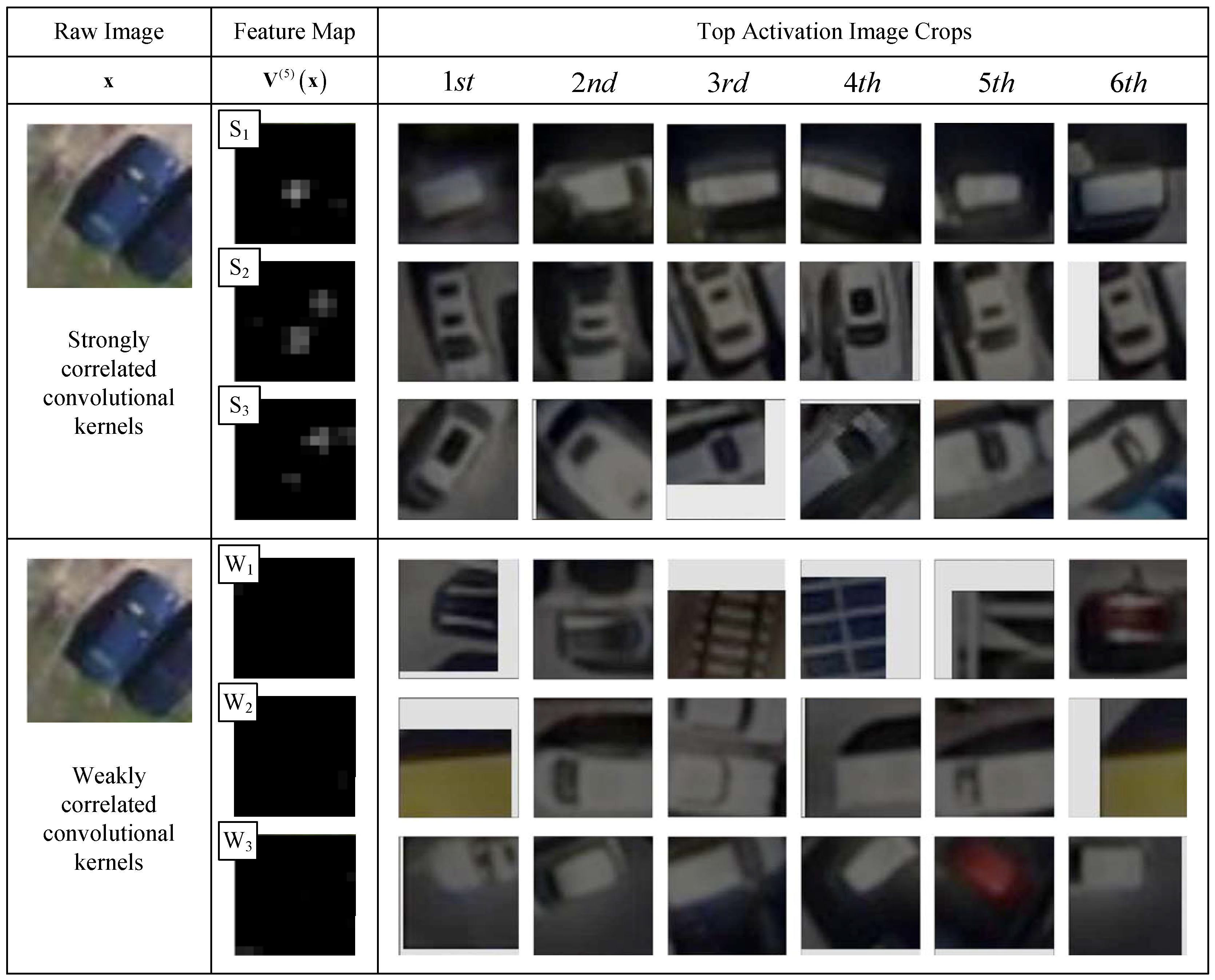
3.2. The Semantic Texture Encoding Pattern for Convolutional Kernels

Despite of all the symbols and equations listed above, studies like [65] sought to produce more interpretable results, helping to better understand and improve the network. One of the important functional components of the DeepVis toolbox proposed in [65] is to find and show the image crops causing the top-most activations by each kernel. This kind of data-centric visualization measure [66,67,68] differs from other means such as deconvolution [69] or image synthesis  [70], showing the correlations between kernel and image samples more directly.
The manifestation effectiveness of the previously mentioned data-centric max-activation illustration method is shown in Figure 2. Therein, six kernels from the CONV5 layer are arranged into two separated groups, denoted as S i i = 1 , 2 , 3 and W i i = 1 , 2 , 3 by their correlation strengths with the input image x shown in the column Raw Image. Under the column Top Activation Image Crops, the max-activation image crops are listed for each kernel, from which a stable image content can be observed, and that represents the textural pattern being encoded. Finally, for each kernel, the correlation between its texture and the input image can be measured by the corresponding feature maps being listed under the Feature Map column. Clearly, the feature maps from the kernels S i have greater activation values, while those belonging to W i are almost black. Considering that these pixel-wise activations will be fed to the trailing fully-connected layers to produce the class-wise likelihoods, strongly activated feature maps from S i indicate that they have stronger correlations with the input image.
In fact, the way in which  the high activations in feature maps from the last convolutional layer help with efficient classification can be exemplified by using Equation (5). Considering two activations h l 1 ( k 1 ) and h l 2 ( k 1 ) at the same position i , m , n from two feature maps Z q 1 ( k 1 ) and Z q 2 ( k 1 ) at layer level k 1 , with that h l 1 ( k 1 ) = Z q 1 , i , m , n ( k 1 ) and h l 2 ( k 1 ) = Z q 2 , i , m , n ( k 1 ) . The connection weights bounded with these two activations are W l 1 ( k ) and W l 2 ( k ) in a single trailing fully-connected layer with its final categorical probabilities generated by transformation z j ( k ) = l W l ( k ) h l + b j ( k ) . Then, by Equation (4), the updating differences for W l 1 , j ( k ) and W l 2 , j ( k ) can be calculated by Equation (7), where g j ( k ) = z j ( k ) J .
W l 1 , j ( k ) = g j ( k ) · h l 1 ( k 1 ) , W l 2 , j ( k ) = g j ( k ) · h l 2 ( k 1 )
So, when there is h l 1 ( k 1 ) > h l 2 ( k 1 ) , greater updating differences will be generated for the W l 1 ( k ) as W l 1 , j ( k ) > W l 2 , j ( k ) . Assuming activations h l 1 ( k 1 ) and h l 2 ( k 1 ) are all beneficial for the final probabilistic estimation on class j, the weighted connection W l 1 ( k ) will grow faster and larger with respect to W l 2 ( k ) . This means that the feature map Z q 1 ( k 1 ) produced by convolutional kernel K q 1 ( k 1 ) is more effective for recognizing samples from class j.

4. Methods

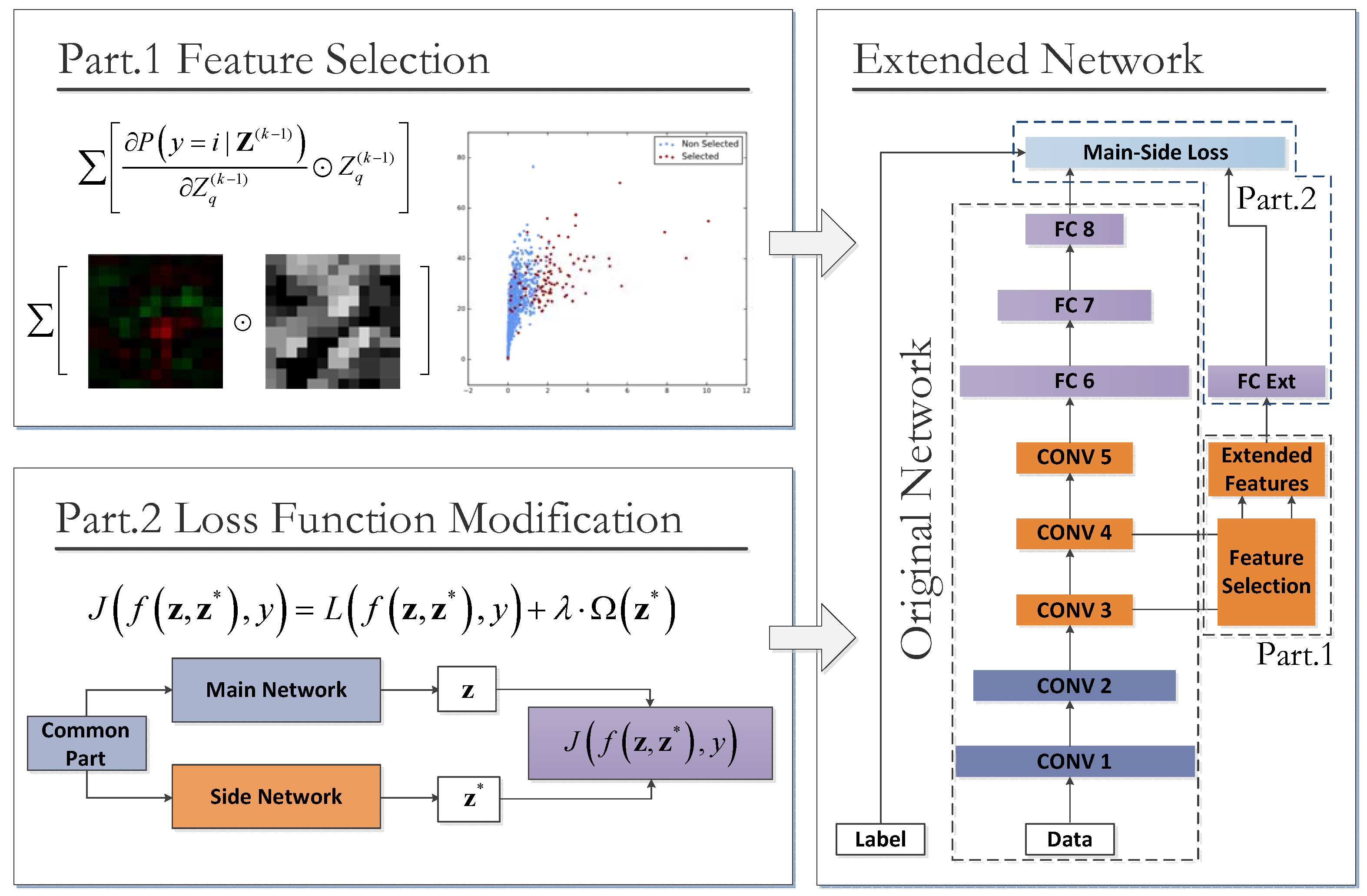
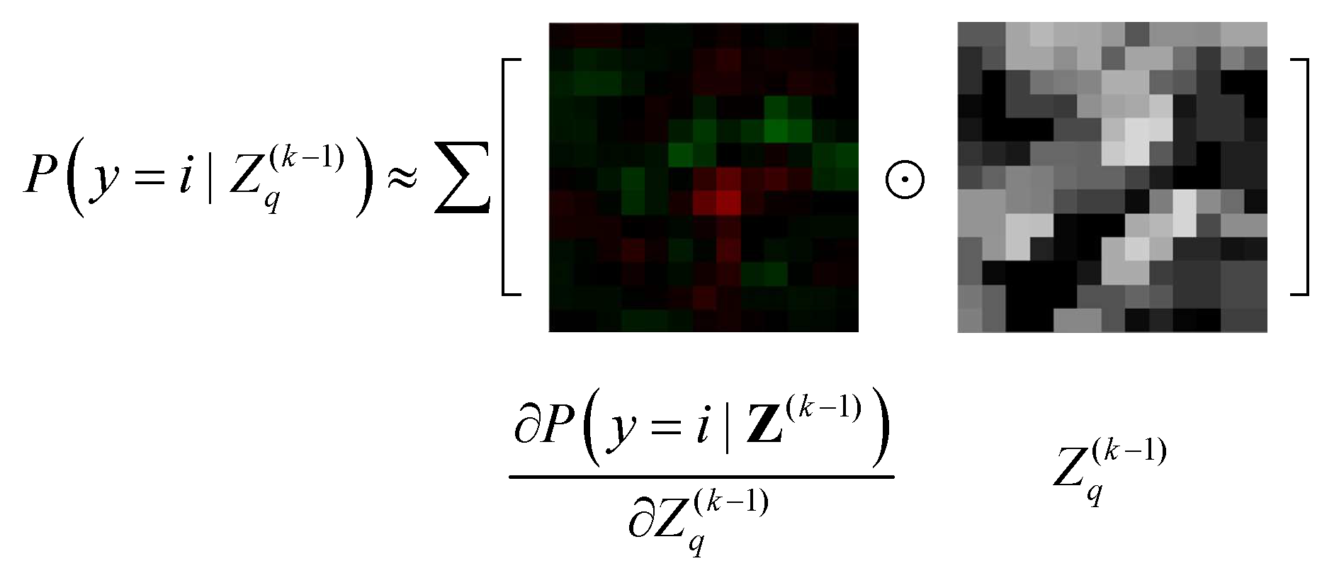
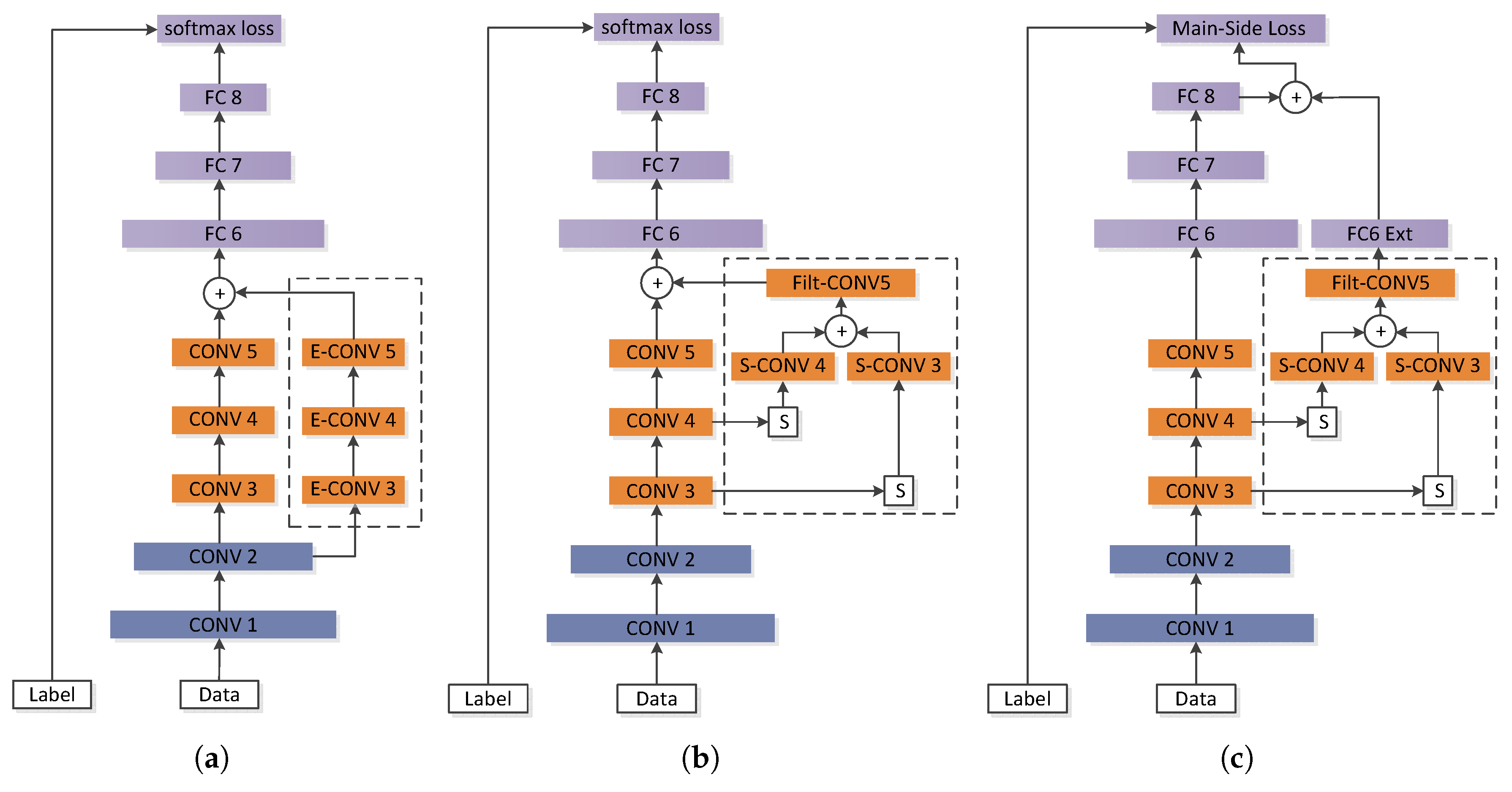
4.1. Overview of the Proposed CNN Extension Scheme

So, being aware of the fact that the modeling power of a CNN is strongly correlated with the diversity of feature maps at the last convolutional layer, this article sets out to tackle the problem of class-imbalance by adopting a cost-effective imbalance-aware feature map extension. Commonly, two kinds of overheads will be introduced when new feature maps are added: the convolution overhead and the connection overhead. Specifically, the convolution overhead refers to the extra convolution operation and extra feature map storage. The connection overhead happens in the fully-connected layer right above the extended convolutional layer, where every connection between pixels in the new feature map and the hidden-neurons in the fully-connected layers should be added. In order to reduce  these two overheads, two general measures are adopted, which are illustrated in Figure 3: (1) the selective feature map extension by a newly derived class-importance measurement; (2) a class-imbalance-sensitive softmax loss function for optimizing the extended component. As a result, after these two modifications, the original network is turned into a bi-partite structure with enhanced sensitivities to the samples in the minority classes.
(1)
Part 1: The selective feature map extension by class-importance measurement. This measure aims to reduce the convolution overhead by reusing feature maps selected from the preceding layers. The criteria adopted in the feature selection process—named feature map class-importance—are similar to that in [58], but are further extended for a multi-class problem with slight modification. Additionally, according to [58], these selected feature maps are further filtered by an extra convolutional layer to reduce noise before being used as the Extended Features component in Figure 3.
(2)
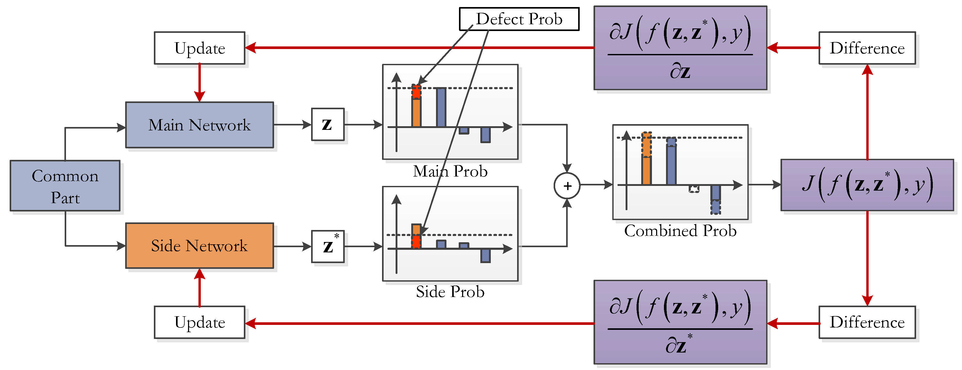
Part 2: the class-imbalance-sensitive softmax loss function. This measure aims at reducing the connection overhead and increasing the class-imbalance awareness of the improved structure. Firstly, the extended network components holding the Extended Features are isolated from the main part of the Original Network by a single-layered fully-connected (FC) layer FC Ext. This FC layer has hidden neurons only as few as the number of output classes; thus, the additional connection quantity for the new maps is largely reduced. Secondly, as shown in the right-most text-box of Figure 3, a new loss function named main-side loss is adopted in place of the original softmax loss to raise the sensitivities of the Extended Features to the minority classes.
For the rest of Section 4, the proposed extension is described in detail based on a network prototype miniature visual geometry group (VGG-M)  shown in Figure 3, which is very similar to AlexNet [71], but has slight improvements on the local convolutional parameters. This illustrative network has five convolutional layers (denoted as CONV1 to CONV5) and three fully-connected layers (denoted as FC6 to FC8), and feature maps for extension are selected from layers CONV3 and CONV4. All of these terms will be used in the following explanations.

4.2. The Network Extension by Selected Feature Maps

The idea of using quadratic expansion of the loss function to reduce less-effective network connections is not new—similar studies can be seen in [72], dating back to 1989. However, loss function-based feature map significance cannot be used to make class related pruning. Instead, the class-wise importance measurement for the feature maps is not hard to obtain—it can be produced by using a similar expansion technique on the output class likelihoods from the output neurons. Considering a general case where Z ( k 1 ) is the collection feature maps at the k 1 th layer generated from input image x , and the predicted probability for class i is P y = i | Z q ( k 1 ) . Then, the contribution of feature map Z q ( k 1 ) to the estimated likelihood on class i can be approximated by Equation (8).
P y = i | Z q ( k 1 ) P y = i | Z ( k 1 ) P y = i | Z ( k 1 ) / q = P y = i | Z ( k 1 ) Z q ( k 1 ) Z q ( k 1 ) + R 2 Z q ( k 1 )
In Equation (8), Z ( k 1 ) / q is the collection of feature maps Z ( k 1 ) without Z q ( k 1 ) , and R 2 Z q ( k 1 ) denotes the other higher-order expansions based on Z q ( k 1 ) . In the first expansion term, P y = i | Z ( k 1 ) Z q ( k 1 ) is the feature map differences back-propagated from the probability value at the ith output neuron, and ⊙ is the element-wise multiplication between matrices. In practice, this difference can be efficiently obtained by back-propagation. By summing the pixel-wise production of the feature map and its differences, the class-importance for the feature map on class i can be obtained. This is vividly shown in Figure 4.
The class-important measure is validated in Figure 5, where the correlations for the maximal feature map activation and maximal feature significance to the probability values on negative samples are presented. Specifically, the x-axis max activations in Figure 5a means the topmost activation value measured from all the feature maps from CONV5. This is also  the case for the x-axis class importance in Figure 5b. As can be seen, the data points in Figure 5b are much tighter and dense, roughly distributed on a curve with shape y = K · x a + x , where a > 0 . Such strong correlation also indicates that the final categorical estimation is mostly based on a single feature map, which again emphasizes the importance of effective feature map selection.
Figure 6a shows the distribution pattern of feature maps from the CONV3 and CONV4 layers in the max class-importance vs. max-activation space. From Figure 6a, it can be determined that  feature maps from the CONV4 are slightly more significant than those from CONV3, with elements in the high class-importance section distributed closer to the x-axis. The categorical inclination of a specific feature map Z q can be calculated by getting the index i of its largest class importance as i = arg max j P y = j | Z q , and their categorical distributions are shown in Figure 6b for five vehicle classes. As can be observed, feature maps belonging to all five classes have similar distributions in the importance section either high and low. Accordingly, in picking the most relevant feature maps for extension, it would be reasonable to select the ones with highest importance scores from each class and control that class-wise quantity according to their classification deficiencies, as in Algorithm 1.
Algorithm 1 Class Imbalance-Aware Extension Feature Map Selection
Input: Classification accuracies ACC j , class-importance P y = i | Z q for feature maps Z q from the CONV3 and CONV4 layers, and the total number of maps to be selected N s e l .
Output: Selected feature map indexes { i } C O N V 3 , C O N V 4 on CONV3 and CONV4
1:
Calculate the number of extension maps needed for each class. For instance, for class j, denote the required extension quantity as N s e l ( j ) , then there is N s e l ( j ) = 1 A C C j i 1 A C C i · N s e l .
2:
For each class j, sort the CONV3 and CONV4 feature maps Z q by their class importance values P y = i | Z q in descending order, with the indexes denoted as m i C O N V 3 , C O N V 4 D E S C ( j ) = m i P y = j | Z m 1 . . . P y = j | Z m N a l l ( k 1 ) , where N a l l = Z q .
3:
For each class j, get the top N s e l ( j ) map indexes from the descending order set as m i C O N V 3 , C O N V 4 T O P N s e l ( j ) = n i i = 1 , . . . , N s e l ( j ) , n i m i C O N V 3 , C O N V 4 D E S C ( j ) .
4:
Merge the class-wise top indexes m i C O N V 3 , C O N V 4 T O P ( j ) from the previous step, and get the output feature map index set as i C O N V 3 , C O N V 4 = j m i C O N V 3 , C O N V 4 T O P N s e l ( j ) .
More specifically, as in Algorithm 1, the selection ratio for each class is measured by their pro rata accuracy deficiencies 1 A C C j i 1 A C C i , so the class-wise selection quantity is N s e l ( j ) = 1 A C C j i 1 A C C i · N s e l . Two exemplified CONV3 and CONV4 feature map selections are illustrated in Figure 7, where the total selection quantities are N s e l = 64 and N s e l = 160 . Therein, the extended feature map candidates mainly reside in the high class-importance region.

4.3. Class Imbalance-Sensitive Softmax Loss Function

Up to the present, explanations for the cost-effective network extension have been focused on the feature map selection process which reduces the convolution overhead. However, the connection overhead is also significant if the newly extended feature maps are encoded directly by the trailing fully-connected layer FC6. Typically, for a network with structure similar to that in Figure 3, there can be as many as 4096 hidden neurons in FC6. Supposing the feature maps from CONV5 are of shape 13 × 13 , then as many as 4096 × 13 × 13 real-valued connection weights will be introduced for every newly added feature map. This kind of overhead can be greatly reduced if these extended feature maps are encoded by a single-layered fully-connected layer independent of the original network, which has hidden neurons with quantity equal to the number of output classes. As shown in Figure 8, the resulting bi-partite network is generalized as composed by three structural components: the common part, the main network, and the side network. For the eight-layered network in Figure 3, the common part refers to the shared layers CONV1 and CONV2, the Main Network refers to layers CONV3 through FC8 in the Original Network, and the Side Network refers to the Extended Features along with the isolated FC Ext layer.
In this structure, the output values from FC Ext can be viewed as an extra categorical estimation based purely on the newly added feature maps, whereas the final categorical prediction from the extended network can be calculated as the summation of these two. Taking the predicted likelihoods from the Main and Side Network components as z and z , this kind of summarization-based likelihood mixture can be viewed as applying a hard connection on these two likelihoods as f z , z = 1 · z + 1 · z , in which both predictions are equally weighted. However, according to the analysis in Section 3.2, this straightforward means does not promise that the extended part will be more correlated with minority class samples. Take the h l ( k 1 ) as some activation from a feature map in the Side Network component at layer k 1 , and its connection weights to a majority class i and a minority class j are denoted as W l , i ( k ) and W l , j ( k ) . Then, according to Equation (9), in the case of using softmax loss, the updating differences g i ( k ) and g j ( k ) from upper layer will be almost equal.
W l , i ( k ) = g i ( k ) · h l ( k 1 ) , W l , j ( k ) = g j ( k ) · h l ( k 1 )
So, in order to achieve class-imbalance sensitivity, the loss function should differ the back-propagated values for the Side Network between majority and minority classes. This setting is manageable. By Figure 8, considering the likelihood summation format as employing the z from Side Network to rectify the estimates z from the Main Network, then the z acts as a filling for the probability deficiencies of z marked by the red bar in Figure 8. Then, if this kind of likelihood amendment is intentionally diminished for the majority classes and encouraged for the minority classes, the predictions from the Side Network are more likely to be correlated with samples from the minority classes.
More specifically, as in Equation (10), the newly introduced Main-Side loss is denoted as J f z , z , y at the right-side of the picture, which takes the softmax loss L f z , z , y as its main component. Then, in order to make these two updating values vary from each other, an extra regularization only relevant with z is added to the loss function, which is denoted as Ω z with a global penalization coefficient λ . Since Ω z is only dependent on the Side Network output z , the back-propagated differences for the Main and Side Network components J f z , z , y z and J f z , z , y z will be different, as in Equation (11).
J f z , z , y = L f z , z , y + λ · Ω z L f z , z , y = log softmax z + z y = i
J f z , z , y z = softmax z + z y = i 1 y = i J f z , z , y z = softmax z + z y = i 1 y = i + λ · Ω z z
Recalling that the softmax loss term L f z , z , y should be diminished during training, this Side Network correlated regularization Ω z should produce small penalty values for the minority classes, but large values for the majority classes. The simplest way to achieve this is to assign varied penalty coefficients for class-wise likelihood values in z , and the classification accuracies for these classes measured on the cross-validation dataset serves such needs. So, as in Equation (12), the additional loss function regularization term Ω z is defined as the Norm-2 of the element-wise multiplication of z and the class-wise accuracies measured on the Main-Network.
Ω z = B z 2 = j β j · z j 2 β j A C C X j , A C C X j = T P X j T P X j + F P X j
The A C C X j in Equation (12) is the averaged accuracy for the given image set X on class j measured by z from the Main Network, B is the categorical penalization coefficient applied on z , and ⊙ means element-wise multiplication between two vectors. Following this definition, for a majority class i already having very high accuracy A C C X i , its penalization will be higher than a minority class j with lower A C C X i , and vice versa. Besides, due to the flexibilities in choosing the set of input images X , three penalization modes can thus be derived, here denoted as Global, Local, and Batch-wise, as shown in Figure 9.
Conceptually, these three penalization modes have specific pros and cons of their own. According to Figure 9, the global penalization β based on the overall sample set O stays unchanged for all training subsets, and thus is insensitive to abnormalities in local space. The local penalization β i , k partially improves the flexibility by using accuracy local cluster S i for each training sample that k belongs to, but such accuracy must still be measured beforehand and could be obsolete during the training. Instead, for the batch-wise mode, a real-time tracking of accuracy can be acquired from the training mini-batch B i , while the additional price is the increased non-linearity in convergence.

5. Experiments and Analysis

5.1. Data Set Description and Experiment Setup

5.1.1. DLR 3K Aerial Image Dataset

The DLR 3K aerial image dataset is an aerial image dataset made publicly available online by the Germany Aerospace Center, which has been studied in [19]. It contains 20 aerial images with resolution of 5616 × 3744 captured over the city of Munich by a low-cost airborne imaging system called DLR 3K+ Cam, which is composed of three non-metric Canon Eos 1Ds Mark III cameras with Zeiss lenses. This system is intended to be fixed on an airplane or a glider with a ZEISS shock mount, where images are taken at the height of 1000 m with real-time ortho-rectification made either on-board or at ground station. All pictures are in RGB real-colored spectral bands (each being digitalized by 8 bits) with ground sampling distance (GSD) at 13 cm.
Although there is no modern skyscraper, these pictures contain quantities of medium-height residential buildings, workshops, trees, lawns, railway track, and streets filled with kinds of vehicles either wide or narrow. All of these put together form a rich set of scenarios which would include most of the typical conditions that cause false detections. Figure 10 shows some of the image samples. The four sub-figures marked as b 1 b 4 are cropped from spots marked by yellow squares in the main image a on the left, which represent classical detection disturbances: tight parking ( b 1 ), shadows from trees and houses ( b 1 , b 2 , and b 3 ), and partial occlusion ( b 4 ). In addition, buildings and man-made facilities in this area have complex textures similar to vehicles, which further increases the localization and categorization difficulties.
Instead of using the original vehicle classes in the dataset, we defined a new set of classes, with the main focus being put on small and medium-sized vehicles; that is, Sedan, Station Wagon (i.e., private SUV), Van, and Working Truck. Quantitative distributions and averaged scales of these vehicle types are listed in Table 1, by which a highly skewed inter-class distribution of samples can be clearly observed. In it, the Station Wagon class has the top-most quantity with the Sedan and Van lagging far behind. The quantity of Working Truck is trivial, with occupation ratios at merely 0.8% in the training set and 0.6% in the testing set.

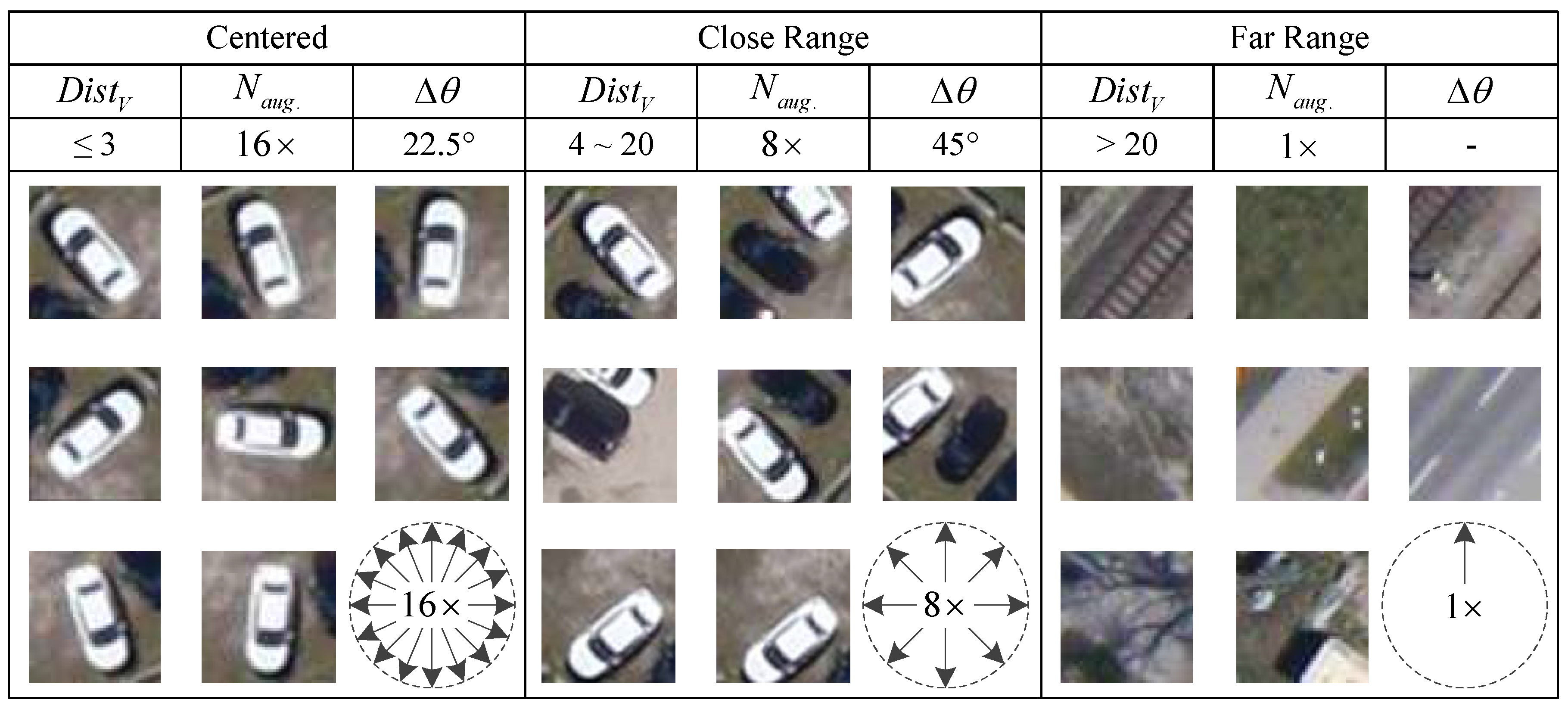
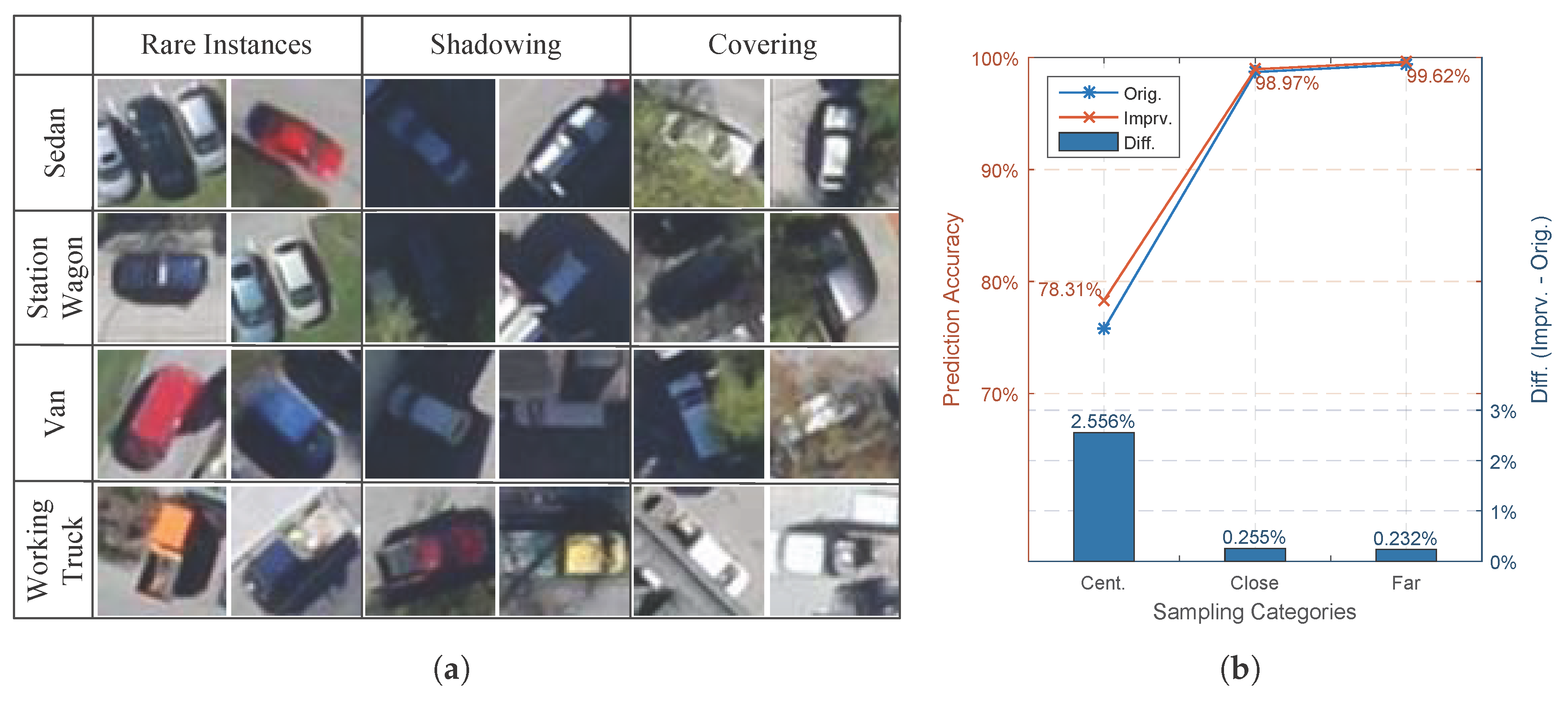
5.1.2. Training and Testing Preparation as a Classification Problem

Since the R-CNN detection structure is employed, it can be regarded as a common CNN-classifier making categorization on full-scaled input images. To facilitate the analysis and verification, 48 × 48 sized patches are uniformly extracted from the original image for a simplified experimental environment. Furthermore, to reduce the quantity of unnecessary negative samples with redundant textural patterns, these image patches are produced from three different regions by their distance to vehicle centers D i s t V , which are shown in Figure 11:
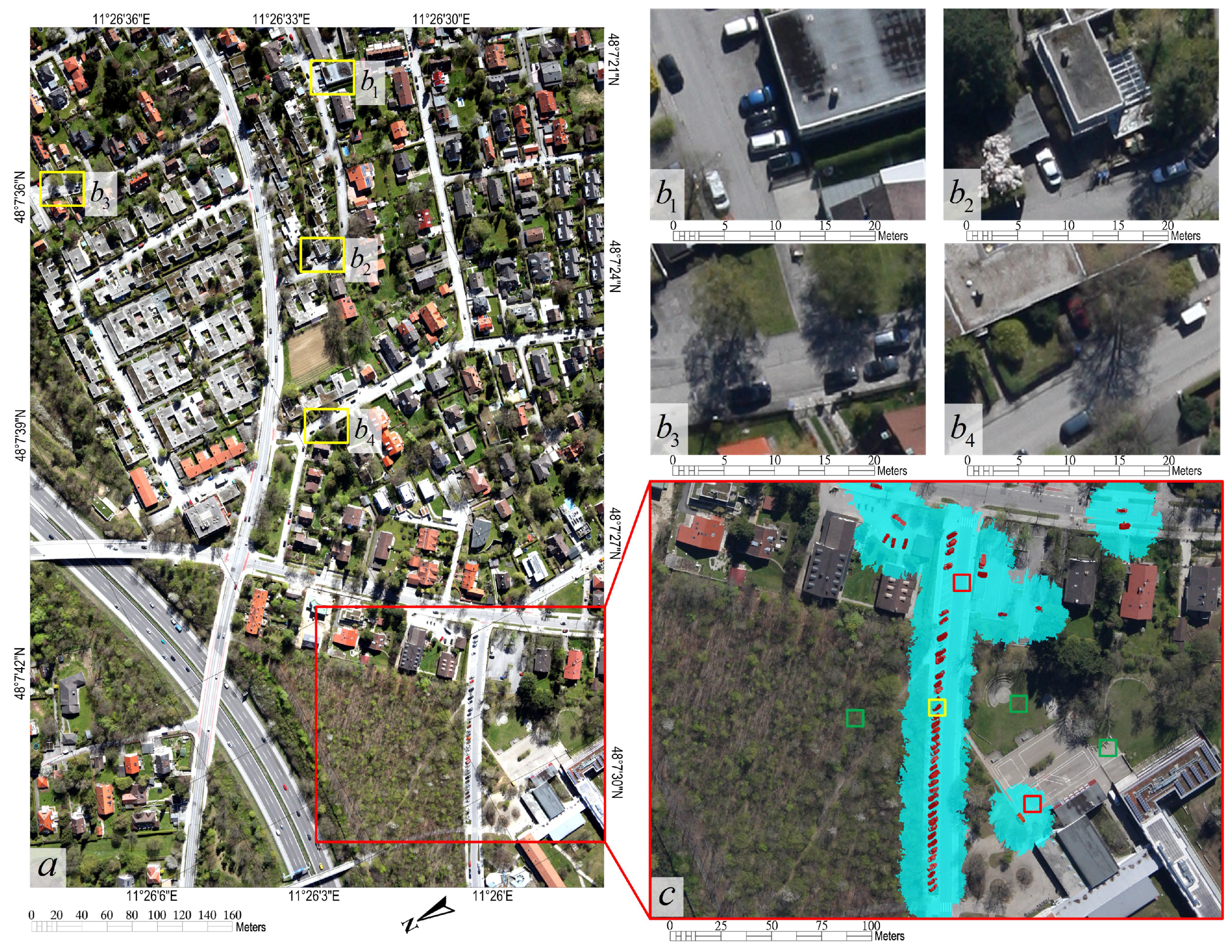
  • The Centered category: position marked by yellow square in sub-figure c in Figure 10 with D i s t V no more than 3 pixels;
  • The Close Range category: positions marked by red squares within the blue shaded region in sub-figure c in Figure 10, whose D i s t V are in range from 4 to 20 pixels;
  • The Far Range category: in sub-figure c from Figure 10, positions marked by green squares outside the blue shaded region with D i s t V more than 20 pixels.
Only samples in the Centered category are treated as positives, which will be further categorized into different vehicle types. Samples from the Close Range and Far Range categories are taken as negatives with different classification difficulties. By Figure 11, data enhancements are performed on these samples by rotation with different times N a u g . , where rotated angle spacing Δ θ is calculated by Δ θ = 360 / N a u g . . Since samples in the Centered and Close Range categories are less populated, their rotate angle spacings are 22 . 5 and 45 with augmentation times at 16 × and 8 × . Finally, sample quantities in these categories are kept equal (approximately 33.3% for each), which results in 210,944 training samples and 534,624 testing samples.

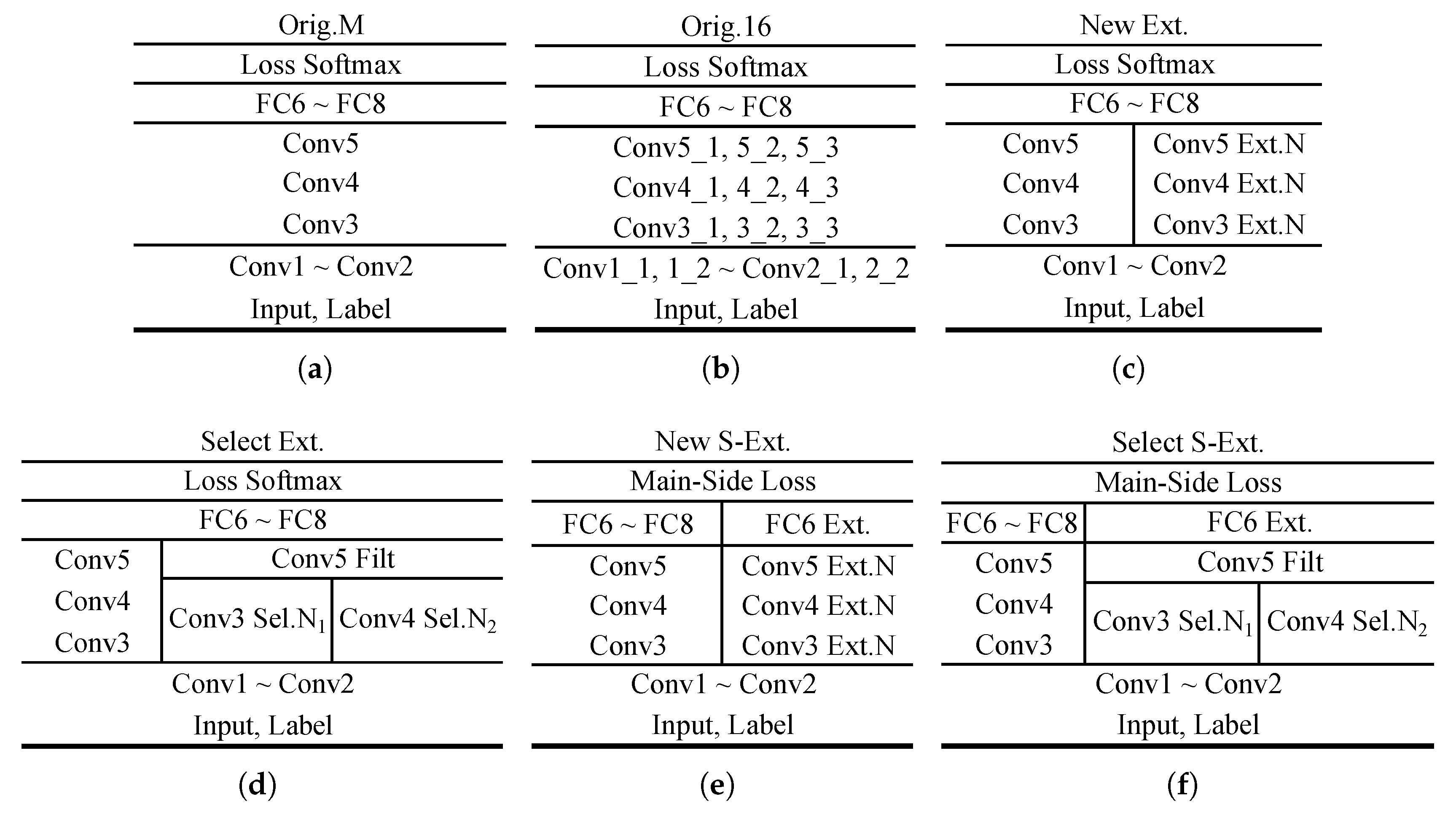
5.1.3. The Baseline Network Structure and Extension Styles for Analysis

To manifest the effectiveness of feature selection and Main-Side loss-based fine-tuning, the VGG-M [74] network is employed as the baseline for the optimized extension. The VGG-M and its full version the 16-layered VGG [75] are powerful holistically structured networks, and have achieved a top-5 error at only 13.7% and 7.4% on the ILSVRC-2012-val dataset, which are the best scores until 2014. Different from its ancestor AlexNet [71], VGG-M uses small kernels of size 3 × 3 with 1 pixel-sized padding, making them ideal for encoding the local structural differences. After that, the development on CNN have either sought greater depth by shortcut connection [76,77,78] or more miscellaneous structural complexities [21,50,79].
Three typical kinds of extension structures based on VGG-M are illustrated in Figure 12, which will be studied in the following subsections. Figure 12a shows the case when the network is extended with blank randomly initialized kernels, and Figure 12b shows the case when selected feature maps from the preceding layers are used for extension. Figure 12c shows the case when both the feature selection and Main-Side loss techniques are employed for extension.
During the experimental analysis in the rest of the section, six kinds of network extension in total are involved for general or specific analysis, and their principle structures are shown in tables in Figure 13. Therein, the miniature VGG-M and full-sized VGG-16 are abbreviated as Orig.M and Orig.16 in Figure 13a,b. Plain network extension by blank kernels and selected feature maps with the original softmax loss are abbreviated as New Ext. and Select Ext., shown by Figure 13c,d. Blank kernel-based and selected feature map-based extension with the class-imbalance-sensitive Main-Side loss are denoted as New S-Ext. and Select S-Ext., shown by Figure 13e,f.
More specifically, the network structures Orig.M, Orig.16, New Ext., Select Ext., and Select S-Ext. with the three penalization modes are compared and studied in Section 5.2 for a holistic comparison. After that, the structures New Ext. and Select Ext. are compared in Section 5.3 to showcase the effect of using selected features in the plain softmax loss-based network extension instead of the blank kernels. Finally, the main factors including the coefficient λ , coefficients B , and the three penalization modes are compared based on the New S-Ext. structure to analyze the behavior of the Main-Side loss function in Section 5.4.

5.2. Experimental Results

The proposed network extension scheme is verified in this section. The networks chosen for comparison are the baseline VGG-M (Orig.M), the 16-layered full-sized VGG (Orig.16), extensions based on the softmax loss (New Ext. and Sel. Ext.), and extensions based on the selected features and Main-Side loss (Sel. S-Ext.).
The parameter model file sizes, memory consumption sizes, and their overheads are shown in Table 2, in which the memory consumption is measured with batch size 96. All data are measured based on the Caffe CNN platform. Generally, Main-Side loss-based network extensions have the least overhead compared to those using softmax loss. The parameter file size increments are trivial since the FC6 Ext. layer has only five hidden neurons. For the memory consumptions, extra memory space saving is done by reusing existing feature maps from preceding layers. Moreover, there are also implicit computation savings by eliminating the convolutions in layers Conv3 Ext. and Conv4 Ext..
Class-wise classification performances measured by accuracies and F1 scores are presented in Table 3 and Table 4, based on extensions with N s e l = 128 and N s e l = 256 by Algorithm 1. In them, the global, local and batch-wise based penalization modes for Select S-Ext. are abbreviated as Glb., Lcl., and Bat.. Due to the limitation of page space, the Select Ext. is further abbreviated as Sel. Ext.. The trailing keyword ReLU indicates the usage of ReLU layer to constrain the Side-Network probabilities. In each column, the first-, second-, and third-highest scores are marked by bold, underline, and double-underline.
From these two tables, several important phenomena need to be taken care of. Firstly, compared to the small version Orig.M, the full-sized Orig.16 is superior in achieving high F1 scores and high accuracy for recognizing negatives, but it is bad for making accurate predictions on the positive classes. This means that the depth-based network extension is more likely to be affected by the class-imbalance. Secondly, the softmax loss-based Sel Ext. has more high scores when N s e l = 128 , meaning that selected features are better utilized for minority classes under smaller extension quantity. Thirdly, the Main-Side loss-based selective feature map extensions are stabler at maintaining high performance for the minority classes (Sedan, Van) except for ones too trivial in size (Working Truck). Fourthly, the usage of ReLU slightly decreases the improvement in accuracies while helping with the enhancement of F1 score. Considering the small overhead cost for the Select S-Ext. variants, their network extension efficiencies are better than the others.
Finally, a brief illustration of the effectiveness of the proposed network extension is given in Figure 14, where Orig.M and Select S-Ext. with N s e l = 256 and λ = exp 2 are chosen for comparison. In Figure 14a, newly recognized images by Select S-Ext. are listed in Figure 14a by their types in each row. According to the common characteristics in appearance, three categories can be established in the columns: those with rare structures or confusing appearances (Rare Instances), those being blurred by shadows (Shadowing), and those being partially covered by trees and buildings (Covering). These are the challenging conditions to which the extended network structure is devoted. At last, prediction accuracies of Orig.M and Select S-Net. on the three sample categories discussed in Section 5.1.2 are illustrated in Figure 14b, abbreviated as Orig. and Imprv.. Therein, accuracy values of Imprv. are marked above its curve markers, and the improvement values Diff. are shown as bars. As expected, samples with greater vehicle center distances (Far Distance) are better predicted by their recognition easiness. Additionally, consistent with the design pattern of Main-Side Loss, greater improvement happens on positives in the Centered category.

5.3. Network Extension Efficiency by Selected Feature Maps

This sub-section discusses the network extension efficiency in using the selected convolutional feature maps. To justify the comparisons, only the extensions New Ext. and Select Ext. based on the softmax loss are adopted, so all kernels will be penalized equally over different classes.
Table 5 shows the classification accuracies between the original VGG-M network and its two extended counterparts, New Ext. and Select Ext.. Seven extension quantities are involved in the comparison, ranging from 64 to 256. Since the feature maps selection scheme described in Algorithm 1 will introduce duplications, the number of feature maps used in the selective extension is always smaller. As can be observed from Table 5, outperforming instances frequently occur on large and medium-sized classes (e.g., Sedan and Station Wagon) which have occupation ratios at 23.06% and 66.96%. For class Van, which has an occupation ratio of 9.10%, only one outperforming is detected. Accuracy differences on class Working Truck fluctuate radically, a class which has the smallest data occupation ratio at 0.88%.
The phenomenon mentioned above can be regarded as the equal penalization nature of the softmax loss. As most of the feature maps selected by Algorithm 1 have high class-significance for all classes, they are more likely to be assigned to majority classes. For the kernels only efficient on minority classes, fluctuations occur as softmax loss attempts to bias them to the majority ones. As a result, poor overall performance refinement is obtained by Select Ext.. As in Figure 15, averaged F1 scores and accuracies are shown for the three networks, with differences between Select Ext. (Select) and New Ext. (Simple) displayed as bars Diff.. Instances where Select Ext. is comparable to New Ext. are marked by arrows, and values for Select Ext. are listed above the markers. For the aforementioned reasons, these instances are rare, and the superiorities of Select Ext. are less significant.
Finally, in Figure 16, a more fair comparison for showing the feature map extension efficiency is performed based on a per-kernel evaluation, where the increase in F1 score for each newly added feature map is calculated by F 1 e x t F 1 o r i g / N e x t , in which F 1 o r i g and F 1 e x t for the baseline and extended network, and N e x t is the number of extended feature maps. As can be observed from Figure 16, the selective feature map-based extension is more efficient in medium-sized minority classes (Sedan and Van) for small extension quantity, while dropping more rapidly than the blank kernel-based one since the selected ones lack enough flexibility.

5.4. Main Factors in Main-Side Loss Function-based Fine-Tuning

Three major configurations have to be considered when using the Main-Side loss to fine-tune the bi-parted Main-Side network, which will be analyzed on the New S-Ext. extension: the first one is whether to fix the FC layers in the Main Network during the fine-tuning; the second one is the penalization coefficient λ and the positive constraint imposed on the single layered FC6 Ext. by an extra ReLU layer; and the third one is the three penalization modes. The reason for choosing the New S-Ext. extension for inspection is that it uses feature maps generated by blank kernels, which ensures that all extended kernels are equally flexible, and thus can be useful for an objective illustration of the impact caused by different configurations.
The first configuration—which involves partial fixation or joint optimization—determines whether the FC6 to FC8 layers should be updated during the fine-tuning. This configuration is only examined on the global penalization version of New S-Ext., with the class-wise performances shown in Table 6. It is then obvious from the table that the joint optimization settings outperform the partially fixed ones in almost every class, including the accuracies and F1 scores, except the trivially populated class Working Truck. The superiority in performance for the joint optimization version is caused by the simultaneous adjustment of the estimation accuracies by the Main Network component, which means that kernels in the Main and Side Networks are optimally re-assigned. It is worth note that the existence of the positive constraint by ReLU layer is less significant for the joint optimization versions, in which the scores are almost identical.
For the second configuration involving the coefficient λ and the positive constraint ReLU, comparing results are shown in Figure 17 and Figure 18. As can be observed from Figure 17a, the influences of λ are more correlated with the prediction accuracies, as they arise when the coefficient decreases. This is because smaller penalization encourages larger likelihood rectifications from the Side Network. This rectification effect is more clear in Figure 18, where medium-sized minority classes (e.g., class Sedan and Van) have greater accuracy improvements compared with majority ones (e.g., Station Wagon). However, the class that is too small (e.g., Working Truck) seems to benefit less from this effect because of the possibility of over-fitting.
In contrast, as seen previously in both figures, the existence of the ReLU layer has little or no influence on the resulting accuracies, while the removal of the ReLU layer seems to help stabilize the fluctuations in accuracies and F1 scores as the penalization λ changes. This is reasonable, since by permitting negative adjustments from the Side Network, they help with pruning the Main Network likelihoods too high to cause over-fitting.
For the third configuration—which involves the comparison between the three penalization modes (Global, Local, and Batch-wise)—experimental results are presented in Table 7. Judging from the scores, there is no apparent winner: Batch-wise penalization is more suitable for improving the small-sized classes (e.g., Working Truck), the Global penalization is more suitable for medium-sized classes (e.g., Sedan and Van), and the Local penalization performs better for the large and medium-sized ones (e.g., Station Wagon and Sedan).

6. Discussion

As mentioned in Section 1, few articles have been found to address the class-imbalance issue in high-resolution aerial image-based vehicle localization and categorization using CNN structure extension; this article serves as an exploration of such methods. A principally similar work named hierarchical deep CNN (HD-CNN) [50] has studied the effectiveness of a tree-structured CNN ensemble on general object classification problems involving dozens of classes. However, with only a few classes, it is inconvenient to build multi-level class taxonomy, and appending a near-full-sized CNN structure might not be sufficiently cost-efficient considering the size of the problem.
The effectiveness of the proposed extension scheme is exemplified in a moderately-sized VGG-M network in a self-proven manner. According to the analysis in the previous experimental section, several general conclusions can be drawn on the network extension-based class-imbalance dealing methods, which can be useful for applying the methods on other similar applications:
(a)
According to Table 3 and Table 4, using wider and deeper network structure with plain extension (blank kernels and softmax loss) will generally improve the classification performances on all classes, while using deeper structure will help more with the generalized performance measured by F1 score.
(b)
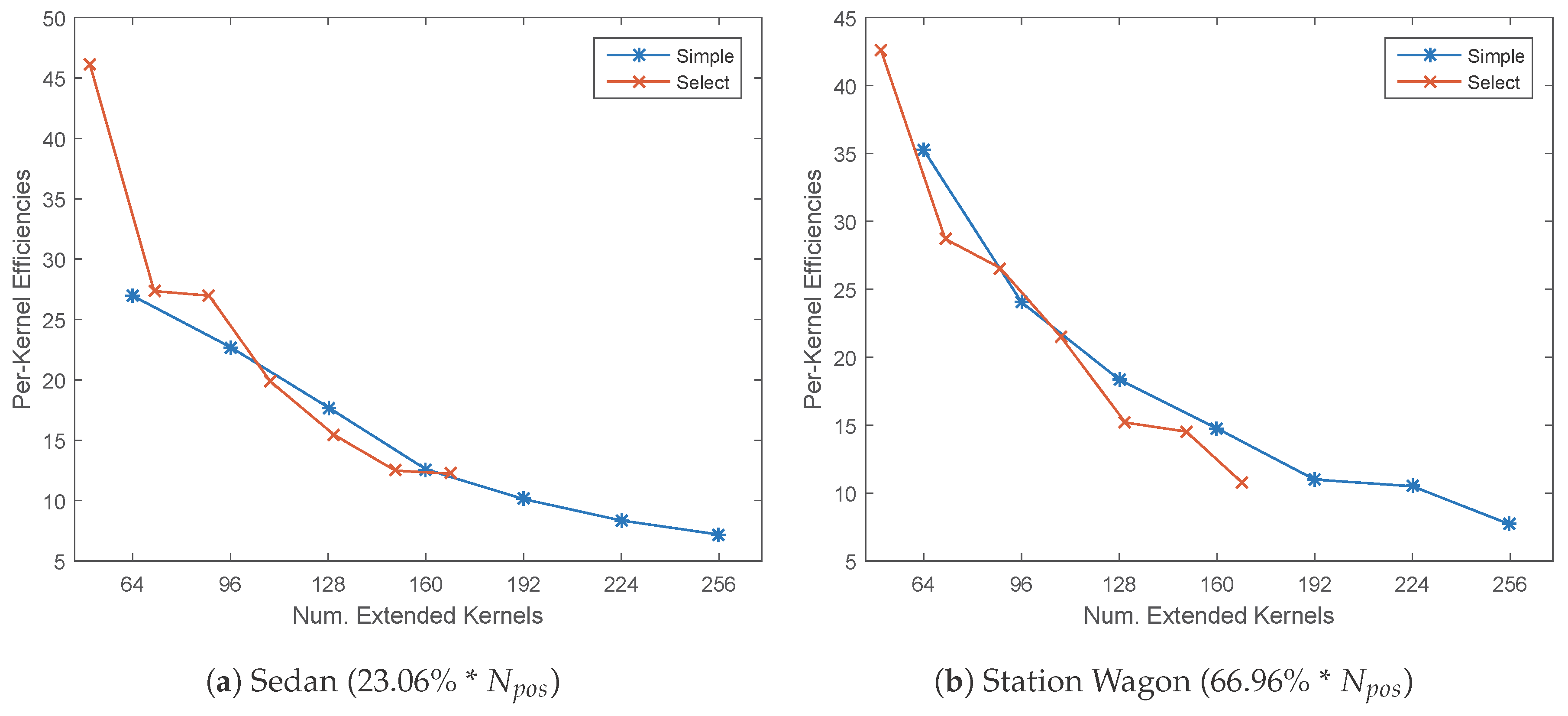
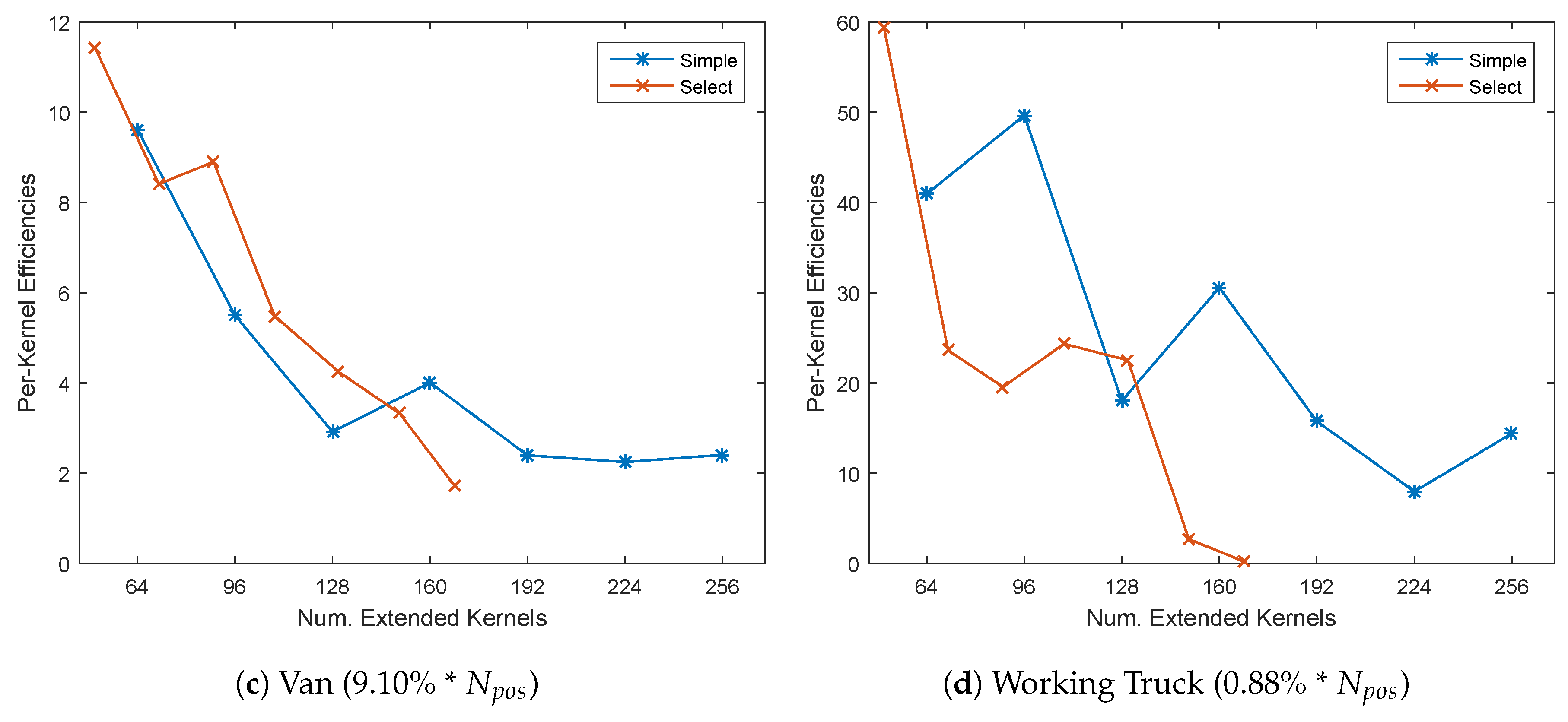
According to Table 5, the effectiveness of the softmax loss-based plain width extension with either blank kernels or selected feature maps will decrease rapidly as the extension quantity increases. Additionally, the selected feature maps are more effective under small extension quantity, while losing their advantage in large extension, as they lack flexibility.
(c)
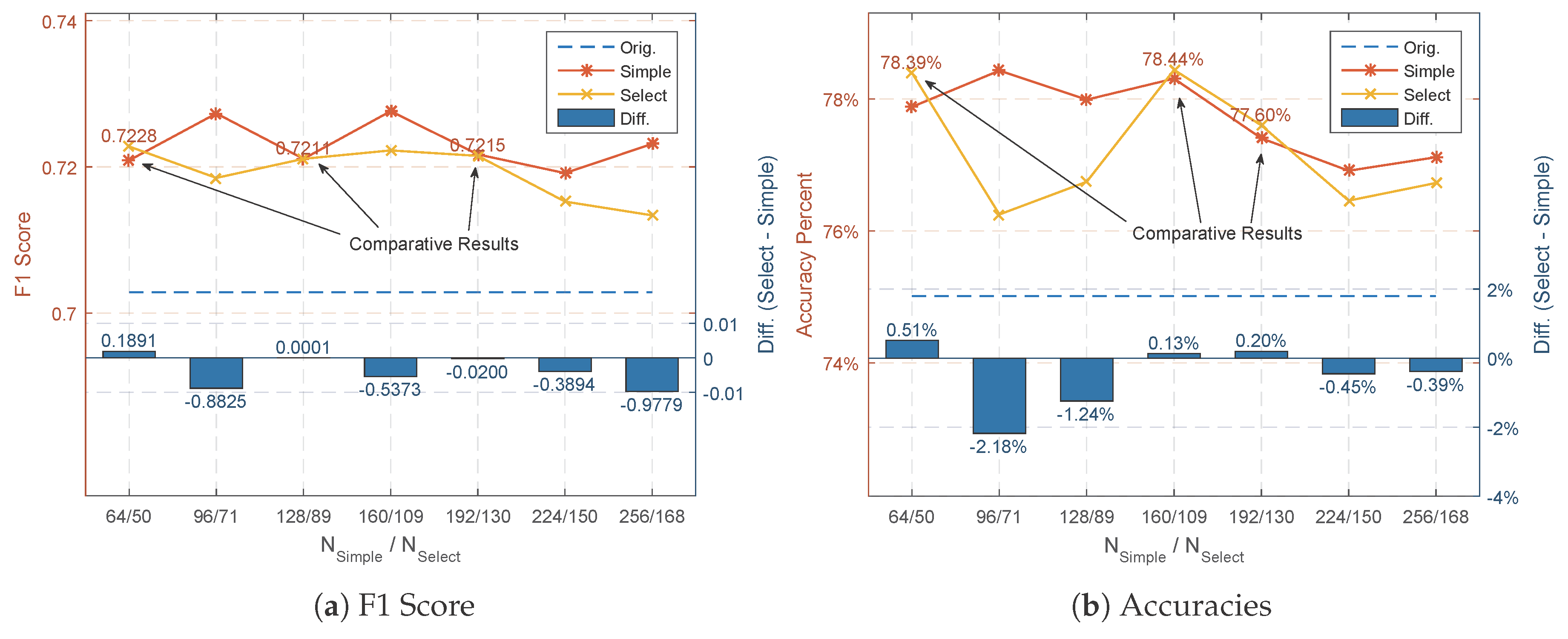
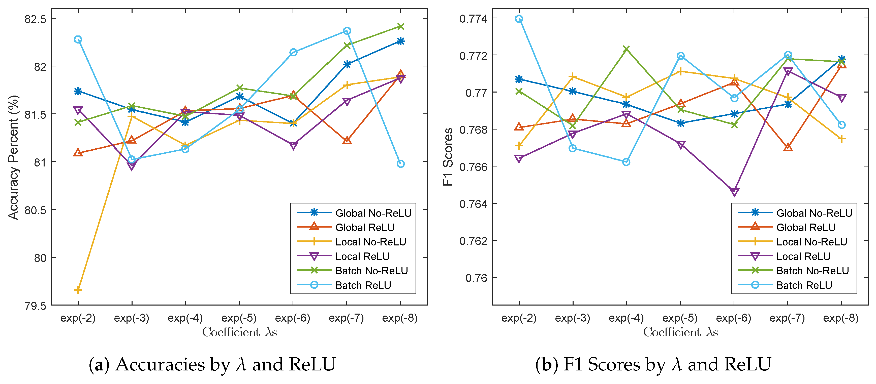
As can be seen from Table 3, Table 4 and Table 5, selected feature maps are more helpful for improving the classification accuracies, while they can barely keep up with the blank kernel-based extension in overall F1 score by Figure 15a. To maintain a reasonably high F1 score performance, the penalization mode Glb.ReLU and Bat.ReLU are preferred, as in Table 3 and Table 4.
(d)
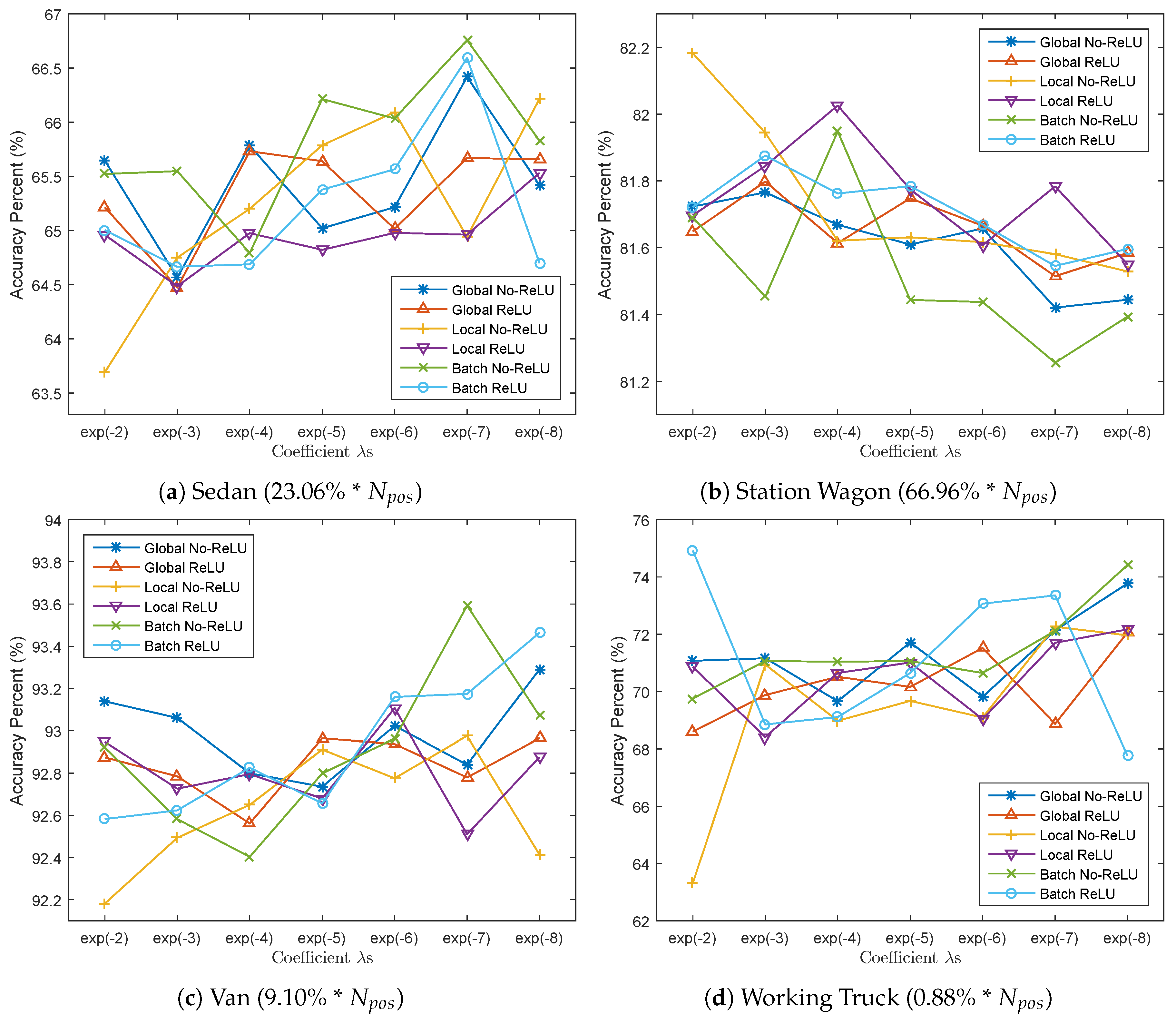
As seen by Figure 17a, penalization modes without ReLU constraint in the Main-Side loss-related fine-tuning can produce a more significant increment in accuracies as the global penalization λ decreases. The existence of a ReLU layer helps to stabilize the fluctuation in F1 scores when λ changes, as in Figure 17b.
(e)
By Figure 18, the class-imbalance-sensitive penalization term Ω z helps to improve the classification accuracies for the medium-sized minority classes (Sedan and Van), but is not so ideal for classes with an absolutely trivial sample quantity (Working Truck).
(f)
The sizes of most effective vehicle classes for the three penalization modes are different. Shown by Table 7, the Global penalization mode is effective on medium-sized classes (Sedan and Van), the Local mode is effective for large- and medium-sized classes (Station Wagon and Sedan), while the Batch-wise mode is effective for small-sized classes (Working Truck).

7. Conclusions

Methods for joint vehicle localization and categorization in aerial images helps with important applications such as traffic flow analysis and suspicious vehicle detection. By treating samples who exceed the permitted location deviation as negatives and classifying them along with the other vehicle classes, the problem of cascaded localization error in separated estimation is eliminated. Top-3 accuracy as high as 99% can be achieved when a typical CNN-based classifier is employed (e.g., the 16-layered VGG network), but it still suffers from the class-imbalance issue, which causes poor classification performances on minority classes.
Based on the R-CNN detection structure, a cost-effective network extension scheme is proposed in this paper to address this issue by introducing less computation and memory consumption overhead. Such efficiency is achieved by two means: the feature map selection and bi-partite Main-Side Network extension, which are performed with the help of a feature map class-importance measurement and a class-imbalance-aware loss function newly proposed in this article. The resulting extended network structure is verified along with its similarly-shaped strong counterparts on a 0.13 m GSD aerial image dataset captured over the urban region of Munich. Experimental results show that the selectively extended feature maps are more effective than those produced by randomly initialized new kernels. By applying the Main-Side loss on this bi-partite network, classification performances on medium-sized minority classes can be further improved. The three Main-Side loss penalizing schemes help with this performance improvement differently, showing varied refinement effect on different-sized classes. Generally, by jointly employing the feature map selection and Main-Side loss optimization schemes, comparable vehicle categorization results can be achieved compared to the counterparts with less parameter and memory overheads.
Key contributions of this study are as follows: First, a novel multi-class feature map importance measurement is proposed by extending the existing significance score for binary classification problems. Second, an easy-to-use cost-effective network extension scheme called Main-Side Network is proposed to greatly improve the classification performances on minority classes with small amount of overhead. Third, three penalization modes are proposed for regularizing the Main-Side loss adopted in this extension, which are simple to implement and beneficial for minority classes with different properties.
In future work, the existing classification deficiencies on tiny classes (e.g., the Working Truck class) is planned to be deeply investigated by using stronger models from the one-class classification. Difficult detection conditions involving shadowed and partially sheltered vehicles caused by skyscrapers and street trees will be further analyzed with harder experimental dataset. Behaviors of the three penalization modes for the Main-Side Loss should be further analyzed in detail to enhance the performance. The Main-Side Network extension structure is intended to be replaced by a network splitting method; thus, the convolution and memory consumption overhead can be completely eliminated.

Acknowledgments

This work is jointly supported by the National Science Foundation of China (NSFC) with granting No. 61302154 and No. 61573350, which mainly focus on aerial image and video analysis. The author would like to acknowledge the editor and reviewers by contributing their precious time to view this article. The authors would also like to thank authors Jason Yosinski et al. in [65] for their selflessness in sharing the great visualization tool.

Author Contributions

Feimo Li designed the experiment and prepared the manuscript; both Hongxing Chang, Shuxiao Li and Chengfei Zhu directed the research project and provided conceptual advices. Xiaosong Lan helped in the revision the manuscript.

Conflicts of Interest

The authors declare no conflict of interest.

Abbreviations

The following abbreviations are used in this manuscript:
ADASYNAdaptive Synthetic Sampling
CBOCluster-based Oversampling
CNNConvolutional Neural Network
DBNDeep Belief Network
FCNFully Convolutional Neural Network
HOGHistogram of Oriented Gradients
GANGenerative Adversarial Network
GSDGround Sampling Distance
LBPLocal Binary Pattern
R-CNNRegions with Convolutional Neural Network Features
ROIRegion of Interest
SIFTScale Invariant Feature Transform
SMOTESynthetic Minority Over-sampling Technique
SVMSupport Vector Machine
t-SNEt-Distributed Stochastic Neighbor Embedding
VGGVisual Geometry Group

References

  1. Xu, Y.; Yu, G.; Wang, Y.; Wu, X.; Ma, Y. A Hybrid Vehicle Detection Method Based on Viola-Jones and HOG + SVM from UAV Images. Sensors 2016. [Google Scholar] [CrossRef] [PubMed]
  2. Tuermer, S.; Kurz, F.; Reinartz, P.; Stilla, U. Airborne vehicle detection in dense urban areas using HoG features and disparity maps. IEEE J. Sel. Top. Appl. Earth Obs. Remote Sens. 2013, 6, 2327–2337. [Google Scholar] [CrossRef]
  3. Hinz, S.; Schlosser, C.; Reitberger, J. Automatic car detection in high resolution urban scenes based on an adaptive 3D-model. In Proceedings of the 2nd GRSS/ISPRS Joint Workshop on Remote Sensing and Data Fusion over Urban Areas, Berlin, Germany, 22–23 May 2003; pp. 167–171. [Google Scholar]
  4. Qu, T.; Zhang, Q.; Sun, S. Vehicle detection from high-resolution aerial images using spatial pyramid pooling-based deep convolutional neural networks. Multimedia Tools Appl. 2016. [Google Scholar] [CrossRef]
  5. Chen, X.; Xiang, S.; Liu, C.L.; Pan, C.H. Vehicle detection in satellite images by hybrid deep convolutional neural networks. IEEE Geosci. Remote Sens. Lett. 2014, 11, 1797–1801. [Google Scholar] [CrossRef]
  6. Cao, L.; Jiang, Q.; Cheng, M.; Wang, C. Robust vehicle detection by combining deep features with exemplar classification. Neurocomputing 2016, 215, 225–231. [Google Scholar] [CrossRef]
  7. Zhu, H.; Chen, X.; Dai, W.; Fu, K.; Ye, Q.; Jiao, J. Orientation robust object detection in aerial images using deep convolutional neural network. In Proceedings of the 2015 IEEE International Conference on Image Processing (ICIP), Quebec City, QC, Canada, 27–30 September 2015; pp. 3735–3739. [Google Scholar]
  8. Qu, S.; Wang, Y.; Meng, G.; Pan, C. Vehicle Detection in Satellite Images by Incorporating Objectness and Convolutional Neural Network. J. Ind. Intell. Inf. 2016. [Google Scholar] [CrossRef]
  9. Girshick, R.; Donahue, J.; Darrell, T.; Malik, J. Rich feature hierarchies for accurate object detection and semantic segmentation. In Proceedings of the IEEE Conference on Computer Vision and Pattern Recognition, Columbus, OH, USA, 23–28 June 2014; pp. 580–587. [Google Scholar]
  10. Girshick, R. Fast r-cnn. In Proceedings of the IEEE International Conference on Computer Vision, Los Alamitos, CA, USA, 7–13 December 2015; pp. 1440–1448. [Google Scholar]
  11. Ren, S.; He, K.; Girshick, R.; Sun, J. Faster r-cnn: Towards real-time object detection with region proposal networks. In Proceedings of the Advances in Neural Information Processing Systems, Montréal, QC, Canada, 7–12 December 2015. [Google Scholar]
  12. Liu, W.; Anguelov, D.; Erhan, D.; Szegedy, C.; Reed, S.; Fu, C.Y.; Berg, A.C. SSD: Single shot multibox detector. In European Conference on Computer Vision; Springer: New York, NY, USA, 2016; pp. 21–37. [Google Scholar]
  13. Redmon, J.; Divvala, S.; Girshick, R.; Farhadi, A. You only look once: Unified, real-time object detection. In Proceedings of the IEEE Conference on Computer Vision and Pattern Recognition, Stanford, CA, USA, 27–30 June 2016; pp. 779–788. [Google Scholar]
  14. He, K.; Zhang, X.; Ren, S.; Sun, J. Spatial pyramid pooling in deep convolutional networks for visual recognition. In European Conference on Computer Vision; Springer: New York, NY, USA, 2014; pp. 346–361. [Google Scholar]
  15. Tang, T.; Zhou, S.; Deng, Z.; Zou, H.; Lei, L. Vehicle Detection in Aerial Images Based on Region Convolutional Neural Networks and Hard Negative Example Mining. Sensors 2017. [Google Scholar] [CrossRef] [PubMed]
  16. Wang, Q.; Lin, J.; Yuan, Y. Salient band selection for hyperspectral image classification via manifold ranking. IEEE Trans. Neural Netw. Learn. Syst. 2016, 27, 1279–1289. [Google Scholar] [CrossRef] [PubMed]
  17. Zhang, F.; Du, B.; Zhang, L. Saliency-guided unsupervised feature learning for scene classification. IEEE Trans. Geosci. Remote Sens. 2015, 53, 2175–2184. [Google Scholar] [CrossRef]
  18. Holt, A.C.; Seto, E.Y.; Rivard, T.; Gong, P. Object-based detection and classification of vehicles from high-resolution aerial photography. Photogramm. Eng. Remote Sens. 2009, 75, 871–880. [Google Scholar] [CrossRef]
  19. Liu, K.; Mattyus, G. Fast multiclass vehicle detection on aerial images. IEEE Geosci. Remote Sens. Lett. 2015, 12, 1938–1942. [Google Scholar]
  20. Razakarivony, S.; Jurie, F. Vehicle detection in aerial imagery: A small target detection benchmark. J. Vis. Commun. Image Represent. 2016, 34, 187–203. [Google Scholar] [CrossRef]
  21. Bell, S.; Lawrence Zitnick, C.; Bala, K.; Girshick, R. Inside-outside net: Detecting objects in context with skip pooling and recurrent neural networks. In Proceedings of the IEEE Conference on Computer Vision and Pattern Recognition, Stanford, CA, USA, 27–30 June 2016; pp. 2874–2883. [Google Scholar]
  22. Ma, Z.; Yu, L.; Chan, A.B. Small instance detection by integer programming on object density maps. In Proceedings of the IEEE Conference on Computer Vision and Pattern Recognition, Boston, MA, USA, 7–12 June 2015; pp. 3689–3697. [Google Scholar]
  23. Arteta, C.; Lempitsky, V.; Noble, J.A.; Zisserman, A. Interactive object counting. In European Conference on Computer Vision; Springer: New York, NY, USA, 2014; pp. 504–518. [Google Scholar]
  24. Yuan, Y.; Wan, J.; Wang, Q. Congested scene classification via efficient unsupervised feature learning and density estimation. Pattern Recognit. 2016, 56, 159–169. [Google Scholar] [CrossRef]
  25. He, H.; Garcia, E.A. Learning from imbalanced data. IEEE Trans. Knowl. Data Eng. 2009, 21, 1263–1284. [Google Scholar]
  26. Branco, P.; Torgo, L.; Ribeiro, R. A survey of predictive modelling under imbalanced distributions. arXiv 2015. [Google Scholar]
  27. He, H.; Ma, Y. Imbalanced Learning: Foundations, Algorithms, and Applications; John Wiley & Sons: New York, NY, USA, 2013. [Google Scholar]
  28. Krawczyk, B. Learning from imbalanced data: Open challenges and future directions. Prog. Artif. Intell. 2016, 5, 221–232. [Google Scholar] [CrossRef]
  29. Chawla, N.V.; Bowyer, K.W.; Hall, L.O.; Kegelmeyer, W.P. SMOTE: synthetic minority over-sampling technique. J. Artif. Intell. Res. 2002, 16, 321–357. [Google Scholar]
  30. He, H.; Bai, Y.; Garcia, E.A.; Li, S. ADASYN: Adaptive synthetic sampling approach for imbalanced learning. In Proceedings of the IEEE International Joint Conference on Neural Networks, Hong Kong, China, 1–8 June 2008; pp. 1322–1328. [Google Scholar]
  31. Jo, T.; Japkowicz, N. Class imbalances versus small disjuncts. ACM Sigkdd Explor. Newsl. 2004, 6, 40–49. [Google Scholar] [CrossRef]
  32. Zhou, Z.H.; Liu, X.Y. On Multi-Class Cost-Sensitive Learning. Comput. Intell. 2010, 26, 232–257. [Google Scholar] [CrossRef]
  33. Ting, K.M. A comparative study of cost-sensitive boosting algorithms. In Proceedings of the 17th International Conference on Machine Learning, Stanford, CA, USA, 29 June–2 July 2000. [Google Scholar]
  34. Krawczyk, B.; Woźniak, M.; Schaefer, G. Cost-sensitive decision tree ensembles for effective imbalanced classification. Appl. Soft Comput. 2014, 14, 554–562. [Google Scholar] [CrossRef]
  35. Huang, C.; Li, Y.; Change Loy, C.; Tang, X. Learning deep representation for imbalanced classification. In Proceedings of the IEEE Conference on Computer Vision and Pattern Recognition, Stanford, CA, USA, 27–30 June 2016; pp. 5375–5384. [Google Scholar]
  36. Jeatrakul, P.; Wong, K.W.; Fung, C.C. Classification of imbalanced data by combining the complementary neural network and SMOTE algorithm. In International Conference on Neural Information Processing; Springer: New York, NY, USA, 2010; pp. 152–159. [Google Scholar]
  37. Simpson, A.J. Over-sampling in a deep neural network. arXiv 2015. [Google Scholar]
  38. Goodfellow, I.; Pouget-Abadie, J.; Mirza, M.; Xu, B.; Warde-Farley, D.; Ozair, S.; Courville, A.; Bengio, Y. Generative adversarial nets. In Proceedings of the Advances in Neural Information Processing Systems, Montreal, QC, Canada, 8–13 December 2014; pp. 2672–2680. [Google Scholar]
  39. Khan, S.H.; Bennamoun, M.; Sohel, F.; Togneri, R. Cost sensitive learning of deep feature representations from imbalanced data. arXiv 2015. [Google Scholar]
  40. Cheng, G.; Zhou, P.; Han, J. Rifd-cnn: Rotation-invariant and fisher discriminative convolutional neural networks for object detection. In Proceedings of the IEEE Conference on Computer Vision and Pattern Recognition, Stanford, CA, USA, 27–30 June 2016; pp. 2884–2893. [Google Scholar]
  41. Bertasius, G.; Shi, J.; Torresani, L. Deepedge: A multi-scale bifurcated deep network for top-down contour detection. In Proceedings of the IEEE Conference on Computer Vision and Pattern Recognition, Boston, MA, USA, 7–12 June 2015; pp. 4380–4389. [Google Scholar]
  42. Shen, W.; Wang, X.; Wang, Y.; Bai, X.; Zhang, Z. Deepcontour: A deep convolutional feature learned by positive-sharing loss for contour detection. In Proceedings of the IEEE Conference on Computer Vision and Pattern Recognition, Boston, MA, USA, 7–12 June 2015; pp. 3982–3991. [Google Scholar]
  43. Robinson, J.P.; Shao, M.; Wu, Y.; Fu, Y. Families in the Wild (FIW): Large-Scale Kinship Image Database and Benchmarks. In Proceedings of the 2016 ACM on Multimedia Conference, Amsterdam, The Netherlands, 15–19 October 2016; pp. 242–246. [Google Scholar]
  44. Santos, C.N.d.; Xiang, B.; Zhou, B. Classifying relations by ranking with convolutional neural networks. arXiv 2015. [Google Scholar]
  45. Schroff, F.; Kalenichenko, D.; Philbin, J. Facenet: A unified embedding for face recognition and clustering. In Proceedings of the IEEE Conference on Computer Vision and Pattern Recognition, Boston, MA, USA, 7–12 June 2015; pp. 815–823. [Google Scholar]
  46. Oh Song, H.; Xiang, Y.; Jegelka, S.; Savarese, S. Deep metric learning via lifted structured feature embedding. In Proceedings of the IEEE Conference on Computer Vision and Pattern Recognition, Stanford, CA, USA, 27–30 June 2016; pp. 4004–4012. [Google Scholar]
  47. Wen, Y.; Zhang, K.; Li, Z.; Qiao, Y. A Discriminative Feature Learning Approach for Deep Face Recognition. In Computer Vision—ECCV 2016; Springer International Publishing: Cham, The Netherlands, 2016; pp. 499–515. [Google Scholar]
  48. Chu, J.L.; Krzyak, A. Analysis of feature maps selection in supervised learning using convolutional neural networks. In Canadian Conference on Artificial Intelligence; Springer: New York, NY, USA, 1994; pp. 59–70. [Google Scholar]
  49. Marcu, A.; Leordeanu, M. Dual Local-Global Contextual Pathways for Recognition in Aerial Imagery. arXiv 2016. [Google Scholar]
  50. Yan, Z.; Zhang, H.; Piramuthu, R.; Jagadeesh, V.; DeCoste, D.; Di, W.; Yu, Y. HD-CNN: hierarchical deep convolutional neural networks for large scale visual recognition. In Proceedings of the IEEE International Conference on Computer Vision, Los Alamitos, CA, USA, 7–13 December 2015; pp. 2740–2748. [Google Scholar]
  51. Jaderberg, M.; Simonyan, K.; Zisserman, A.; Kavukcuoglu, K. Spatial transformer networks. In Proceedings of the Advances in Neural Information Processing Systems, Montréal, QC, Canada, 7–12 December 2015. [Google Scholar]
  52. Wang, N.; Li, S.; Gupta, A.; Yeung, D.Y. Transferring rich feature hierarchies for robust visual tracking. arXiv 2015. [Google Scholar]
  53. Ng, W.W.; Zeng, G.; Zhang, J.; Yeung, D.S.; Pedrycz, W. Dual autoencoders features for imbalance classification problem. Pattern Recognit. 2016, 60, 875–889. [Google Scholar] [CrossRef]
  54. Guyon, I.; Gunn, S.; Nikravesh, M.; Zadeh, L.A. Feature Extraction: Foundations and Applications; Springer: New York, NY, USA, 2008. [Google Scholar]
  55. Bar, Y.; Diamant, I.; Wolf, L.; Lieberman, S.; Konen, E.; Greenspan, H. Chest pathology identification using deep feature selection with non-medical training. Comput. Methods Biomech. Biomed. Eng. Imaging Vis. 2016. [Google Scholar] [CrossRef]
  56. Matsugu, M.; Cardon, P. Unsupervised feature selection for multi-class object detection using convolutional neural networks. In Advances in Neural Networks—ISNN 2004; Springer: New York, NY, USA, 2004; pp. 864–869. [Google Scholar]
  57. Zou, Q.; Ni, L.; Zhang, T.; Wang, Q. Deep Learning Based Feature Selection for Remote Sensing Scene Classification. IEEE Geosci. Remote Sens. Lett. 2015, 12, 2321–2325. [Google Scholar] [CrossRef]
  58. Wang, L.; Ouyang, W.; Wang, X.; Lu, H. Visual tracking with fully convolutional networks. In Proceedings of the IEEE International Conference on Computer Vision, Los Alamitos, CA, USA, 7–13 December 2015; pp. 3119–3127. [Google Scholar]
  59. Liu, D.R.; Li, H.L.; Wang, D. Feature selection and feature learning for high-dimensional batch reinforcement learning: A survey. Int. J. Autom. Comput. 2015, 12, 229–242. [Google Scholar] [CrossRef]
  60. Yang, B.; Yan, J.; Lei, Z.; Li, S.Z. Convolutional channel features. In Proceedings of the IEEE International Conference on Computer Vision, Los Alamitos, CA, USA, 7–13 December 2015; pp. 82–90. [Google Scholar]
  61. Zhong, B.; Zhang, J.; Wang, P.; Du, J.; Chen, D. Jointly Feature Learning and Selection for Robust Tracking via a Gating Mechanism. PLoS ONE 2016, 11, e0161808. [Google Scholar] [CrossRef] [PubMed]
  62. Goodfellow, I.; Bengio, Y.; Courville, A. Deep Learning; MIT Press: Cambridge, MA, USA, 2016; pp. 166–373. [Google Scholar]
  63. Jarrett, K.; Kavukcuoglu, K.; LeCun, Y.; Ranzato, M. What is the best multi-stage architecture for object recognition? In Proceedings of the 2009 IEEE 12th International Conference on Computer Vision, Kyoto, Japan, 29 September–2 October 2009; pp. 2146–2153. [Google Scholar]
  64. Nair, V.; Hinton, G.E. Rectified linear units improve restricted boltzmann machines. In Proceedings of the 27th International Conference on Machine Learning (ICML-10), Haifa, Israel, 21–25 June 2010; pp. 807–814. [Google Scholar]
  65. Yosinski, J.; Clune, J.; Nguyen, A.; Fuchs, T.; Lipson, H. Understanding neural networks through deep visualization. arXiv 2015. [Google Scholar]
  66. Simonyan, K.; Vedaldi, A.; Zisserman, A. Deep inside convolutional networks: Visualising image classification models and saliency maps. arXiv 2013. [Google Scholar]
  67. Nguyen, A.; Yosinski, J.; Clune, J. Deep neural networks are easily fooled: High confidence predictions for unrecognizable images. In Proceedings of the IEEE Conference on Computer Vision and Pattern Recognition, Boston, MA, USA, 7–12 June 2015; pp. 427–436. [Google Scholar]
  68. Szegedy, C.; Zaremba, W.; Sutskever, I.; Bruna, J.; Erhan, D.; Goodfellow, I.; Fergus, R. Intriguing properties of neural networks. arXiv 2013. [Google Scholar]
  69. Zeiler, M.D.; Fergus, R. Visualizing and understanding convolutional networks. In European Conference on Computer Vision; Springer: New York, NY, USA, 2014; pp. 818–833. [Google Scholar]
  70. Erhan, D.; Bengio, Y.; Courville, A.; Vincent, P. Visualizing Higher-Layer Features of a Deep Network. Univ. Montr. 2009, 1341, 3. [Google Scholar]
  71. Krizhevsky, A.; Sutskever, I.; Hinton, G.E. Imagenet classification with deep convolutional neural networks. In Proceedings of the Advances in Neural Information Processing Systems, Lake Tahoe, ND, USA, 3–6 December 2012; pp. 1097–1105. [Google Scholar]
  72. LeCun, Y.; Denker, J.S.; Solla, S.A.; Howard, R.E.; Jackel, L.D. Optimal Brain Damage; NIPs: Tokyo, Japan, 1989; Volume 2, pp. 598–605. [Google Scholar]
  73. Maaten, L.v.d.; Hinton, G. Visualizing data using t-SNE. J. Mach. Learn. Res. 2008, 9, 2579–2605. [Google Scholar]
  74. Chatfield, K.; Simonyan, K.; Vedaldi, A.; Zisserman, A. Return of the devil in the details: Delving deep into convolutional nets. arXiv 2014. [Google Scholar]
  75. Simonyan, K.; Zisserman, A. Very deep convolutional networks for large-scale image recognition. arXiv 2014. [Google Scholar]
  76. He, K.; Zhang, X.; Ren, S.; Sun, J. Deep residual learning for image recognition. In Proceedings of the IEEE Conference on Computer Vision and Pattern Recognition, Stanford, CA, USA, 27–30 June 2016; pp. 770–778. [Google Scholar]
  77. Huang, G.; Liu, Z.; Weinberger, K.Q.; van der Maaten, L. Densely connected convolutional networks. arXiv 2016. [Google Scholar]
  78. Targ, S.; Almeida, D.; Lyman, K. Resnet in Resnet: Generalizing residual architectures. arXiv 2016. [Google Scholar]
  79. Szegedy, C.; Liu, W.; Jia, Y.; Sermanet, P.; Reed, S.; Anguelov, D.; Erhan, D.; Vanhoucke, V.; Rabinovich, A. Going deeper with convolutions. In Proceedings of the IEEE Conference on Computer Vision and Pattern Recognition, Boston, MA, USA, 7–12 June 2015; pp. 1–9. [Google Scholar]
Figure 1. A typical convolutional neural network (CNN) structure, with feature and difference maps produced by the forward and backward propagations. SW: station wagon; WT: working truck.
Remotesensing 09 00494 g001
Figure 2. Illustration of the semantic meaning of the convolutional kernels. The raw input image is displayed in the Raw Image column; the six feature maps produced by six different kernels at the CONV5 layer are shown in the Feature Map column; and six arrays of local image crops on which the top six feature map activations are produced are shown in the Top Activation Image Crops column.
Remotesensing 09 00494 g002
Figure 3. The general structure of the proposed network enhancement method.
Remotesensing 09 00494 g003
Figure 4. The first-order term of the Taylor expansion in Equation (8). P y = i | Z ( k 1 ) Z q ( k 1 ) denotes the feature map difference, positive, negative, and zero values marked as green, red, and black.
Remotesensing 09 00494 g004
Figure 5. Correlations of the max-activations and class-importance with the class probability of the negative class. (a) Max-activation vs. class probability. (b) Max class-importance vs. class probability.
Remotesensing 09 00494 g005
Figure 6. Scatter plots showing the distribution of the feature maps Z q from CONV3 and CONV4 in the class-importance vs. max-activation space. (a) The distributions of CONV3 and CONV4 feature maps. (b) Feature maps correlated to the five classes by the class-importance measurement.
Remotesensing 09 00494 g006
Figure 7. (a) The 50 selected maps for N s e l = 64 . (b) The 109 selected maps for N s e l = 160 .
Remotesensing 09 00494 g007
Figure 8. Principle structure of the class-imbalance aware Main-Side Network.
Remotesensing 09 00494 g008
Figure 9. The t-Distribution stochastic neighbor embedding (t-SNE) -based visualization [73] of the negatives and vehicle types in the FC8 output space, and the three penalization modes used for B : (a) global, (b) local, and (c) batch-wise.
Remotesensing 09 00494 g009
Figure 10. (a) A typical frame from the training sample. ( b 1 b 4 ) Typical difficult detection cases. (c) The close-to-vehicle region (shaded blue) and categorical sampling positions.
Remotesensing 09 00494 g010
Figure 11. The sample categories used on the three regions: Centered, Close Range, and Far Range.
Remotesensing 09 00494 g011
Figure 12. Three typical extension schemes. (a) Plain extension with blank kernel generated feature maps; (b) Plain extension with selected feature maps; (c) Main-Side bi-parted extension with selected feature maps.
Remotesensing 09 00494 g012
Figure 13. The five network structures studied in the experimental section. (a) The baseline network miniature miniature visual geometry group (VGG-M) (Orig.M) and (b) 16-layered VGG (Orig.16), the comparative extensions with either (c,d) the Loss of Softmax (New Ext., Select Ext.) or (e,f) the proposed Main-Side Loss (New S-Ext., Select S-Ext.).
Remotesensing 09 00494 g013
Figure 14. Network classification performance improvement illustrated by the established classification dataset. (a) Newly recognized positives after extension. (b) Prediction accuracies and the increments on sample categories: Centered (Cent.), Close Range (Close), and Far Range (Far).
Remotesensing 09 00494 g014
Figure 15. Overall performance comparisons between the Orig.M, New Ext. and Select Ext. under different extension sizes. (a) the averaged F1 scores, (b) the averaged accuracies. Instances where Select Ext. is comparable to New Ext. are marked by arrows.
Remotesensing 09 00494 g015
Figure 16. Efficiency comparison of extended feature maps (kernels). N p o s is the quantity of all vehicles. Selected feature maps (kernels) are more effective for small extension and minority classes.
Remotesensing 09 00494 g016aRemotesensing 09 00494 g016b
Figure 17. Influences of the coefficient λ and ReLU constraint on the overall accuracy and F 1 score in three modes. (a) the averaged accuracies; (b) the averaged F 1 scores.
Remotesensing 09 00494 g017
Figure 18. Influences of the penalization mode and the coefficient λ on accuracy and F 1 score for different vehicle types. N p o s is the quantity of positives, which is all the vehicles.
Remotesensing 09 00494 g018
Table 1. The vehicle types defined in this paper and the basic statistics.
TypeSamplesTraining SetTesting Set
L (px)W (px)NL (px)W (px)N
Sedan Remotesensing 09 00494 i00121.4510.4777620.8310.161075
Station Wagon Remotesensing 09 00494 i00219.999.76230219.149.324178
Van Remotesensing 09 00494 i00324.6512.0631224.1411.83512
Working Truck Remotesensing 09 00494 i00427.1713.312926.5813.0234
Note: L (px) and W (px) denote the length and width of vehicles in pixels, and N denotes the quantity.
Table 2. Trained model file sizes and GPU-memory consumption for batch size of 96.
Net Struct.Orig.MOrig.16New Ext.
128
New Ext.
256
Sel. Ext.
128
Sel. Ext.
256
Sel. S-Ext.
128
Sel. S-Ext.
256
Model (Mb)361.7537.1439.6519.8426.1460.9362.2362.8
Δ Model (Mb)-175.477.9158.164.499.20.51.1
Mem (Mb)1820.310547.11988.42093.02018.52053.71977.42004.3
Δ Mem (Mb)-8726.8168.0272.7192.7223.1157.1183.9
Table 3. Best averaged F1 score cases of classification performance for 128 feature map extension.
NegativeSedanStation WagonVanWorking Truck
ACCF1ACCF1ACCF1ACCF1ACCF1
Orig.M96.83%0.979158.40%0.624781.81%0.801090.11%0.842269.72%0.5435
Orig.1699.68%0.962457.13%0.643382.04%0.832991.64%0.865070.05%0.5914
New Ext.97.20%0.982263.38%0.647482.13%0.824591.92%0.845974.52%0.5666
Sel. Ext.96.90%0.980863.56%0.648782.25%0.824793.00%0.850168.16%0.5609
Glb.97.01%0.981065.73%0.643881.51%0.830392.38%0.847171.29%0.5377
Glb.ReLU97.22%0.982065.95%0.641081.27%0.831592.69%0.847771.25%0.5406
Lcl.97.00%0.981365.45%0.640881.65%0.831092.66%0.849769.63%0.5418
Lcl.ReLU97.27%0.982364.61%0.640481.53%0.828592.56%0.849870.70%0.5375
Bat.97.12%0.981464.40%0.641781.54%0.827692.89%0.847170.38%0.5351
Bat.ReLU97.30%0.982063.87%0.640781.67%0.827392.66%0.850572.78%0.5556
Note: The first, second and third topmost values in each column are marked by bold, underline and double-underline. Meanings of abbreviations are: the baseline VGG-M (Orig.M), the 16-layered full-sized VGG (Orig.16), the softmax loss based extensions (New Ext. and Sel. Ext.), and Main-Side loss based extensions (Sel. S-Ext.).
Table 4. Best averaged F1 score cases of classification performance for 256 feature map extension.
NegativeSedanStation WagonVanWorking Truck
ACCF1ACCF1ACCF1ACCF1ACCF1
Orig.M96.83%0.979158.40%0.624781.81%0.801090.11%0.842269.72%0.5435
Orig.1699.68%0.962457.13%0.643382.04%0.832991.64%0.865070.05%0.5914
New Ext.97.23%0.982361.97%0.643182.26%0.820792.26%0.848471.97%0.5804
Sel. Ext.96.96%0.980861.98%0.645382.39%0.819291.69%0.845170.85%0.5439
Glb.97.12%0.981664.26%0.641981.47%0.826392.83%0.845370.31%0.5409
Glb.ReLU97.16%0.981864.47%0.644181.80%0.829092.94%0.850573.60%0.5472
Lcl.96.94%0.980965.91%0.638481.45%0.830692.46%0.850768.53%0.5469
Lcl.ReLU97.11%0.981665.11%0.643981.69%0.829692.46%0.848172.05%0.5564
Bat.97.01%0.980963.75%0.641381.52%0.824292.92%0.845769.94%0.5442
Bat.ReLU97.31%0.982365.12%0.642081.45%0.830392.70%0.848271.70%0.5419
Note: The first, second and third topmost values in each column are marked by bold, underline and double-underline. Meanings of abbreviations are: the baseline VGG-M (Orig.M), the 16-layered full-sized VGG (Orig.16), the softmax loss based extensions (New Ext. and Sel. Ext.), and Main-Side loss based extensions (Sel. S-Ext.).
Table 5. Classification accuracies for softmax loss-based extensions New Ext. and Select Ext..
OriginalSedanStation WagonVanWorking Truck
ACC 58.40%ACC 81.81%ACC 90.11%ACC 69.72%
New Ext. & Sel. Ext.NewSelectNewSelectNewSelectNewSelect
N64/S5063.02%63.19%81.85%82.27%92.58%91.81%74.06%76.30%
N96/S7163.00%62.78%82.11%82.35%92.76%91.90%75.84%67.97%
N128/S8963.38%63.56%82.13%82.25%91.92%93.00%74.52%68.16%
N160/S10963.23%63.59%82.07%81.96%92.62%92.48%75.30%75.73%
N192/S13062.55%62.30%81.99%82.40%92.53%92.07%72.54%73.62%
N224/S15063.38%63.10%81.84%82.05%92.46%91.95%69.97%68.73%
N256/S16861.97%61.98%82.26%82.39%92.26%91.69%71.97%70.85%
Note: For each pair of accuracies given by New Ext. and Select Ext., instances where the Select Ext. outperforms the New Ext. are emphasized by bold font.
Table 6. Categorization accuracies for fixed-Main and joint optimization, best average F1 cases.
SedanStation WagonVanWorking Truck
ACCF1ACCF1ACCF1ACCF1
Global No ReLU, Fix-M62.12%0.627581.10%0.821291.46%0.847972.67%0.5492
Global ReLU, Fix-M60.26%0.628981.48%0.813291.03%0.846372.33%0.5542
Global No ReLU, Joint65.42%0.643581.44%0.832093.29%0.849773.77%0.5508
Global ReLU, Joint65.66%0.644981.58%0.832592.96%0.848472.06%0.5490
Note: Fixed and non-fixed optimization settings are abbreviated as Fix-M and Joint, and the top-2 highest scores are marked as bold and underline.
Table 7. Best accuracies and F1s for three modes with or without the ReLU layer on FC6 Ext. layer.
SedanStation WagonVanWorking Truck
ACCF1ACCF1ACCF1ACCF1
Global No ReLU, Joint65.42%0.643581.44%0.832093.29%0.849773.77%0.5508
Global ReLU, Joint65.66%0.644981.58%0.832592.96%0.848472.06%0.5490
Local No ReLU, Joint65.79%0.641581.63%0.833592.91%0.849469.67%0.5491
Local ReLU, Joint65.53%0.644181.55%0.832092.88%0.846872.17%0.5432
Batch-wise No ReLU, Joint64.79%0.644281.95%0.830892.40%0.849871.04%0.5548
Batch-wise ReLU, Joint65.00%0.643581.72%0.830792.58%0.847774.92%0.5662
Note: In each column, the first and second topmost values are emphasized by bold and underline. Implementations with and without ReLU layer are marked by ’ReLU’ and ’No ReLU’. ’Joint’ means non-fixed optimization same as that in Table 6.

