
Characterization of a Highly Biodiverse Floodplain Meadow Using Hyperspectral Remote Sensing within a Plant Functional Trait Framework

 , and
, and
Abstract
:
1. Introduction
2. Background
2.1. MG4 Floodplain Meadows
2.2. Study Area

3. Materials and Methods
3.1. Sampling Locations

| Class | Main Species Found | Date of Spectral Sampling | Number of Sampling Locations |
|---|---|---|---|
| DRY | Sanguisorba officinalis, Centaurea nigra, Succisa pratensis, Galium verum, Lotus corniculatus, Primula veris, Dactylis glomerata, Carex flacca, Festuca rubra, Trisetum flavescens | 5 and 9 July 2013 | 25 (400 spectra) |
| WET | Carex riparia, Carex acuta, Juncus acutiflorus; Filipendula ulmaria, Thalictrum flavum, Lysimachia numullaria, Holcus lanatus, Hordeum secalinum, Cardamine pratensis, Agrostis stolonifera | 5 and 9 July 2013 | 10 (158 spectra) |
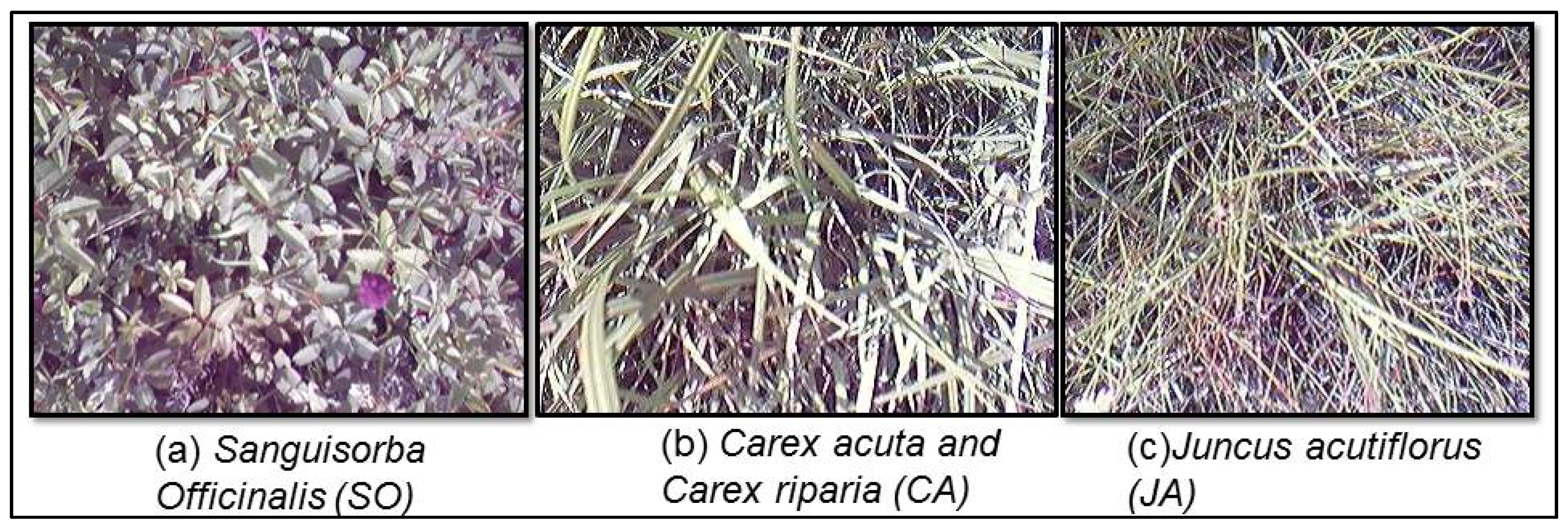
| SO | Sanguisorba officinalis | 12 June 2014 | 8 (131 spectra) |
| CA | Carex acuta, Carex riparia | 13 June 2014 | 10 (146 spectra) |
| JA | Juncus acutiflorus | 12 and 13 June 2014 | 7 (85 spectra) |
3.2. Spectral Sampling, Post Processing and Analysis
3.3. Field Data Collection for Vegetation Biophysical and Functional Properties
3.4. Model Simulations
3.5. Soil Measurements
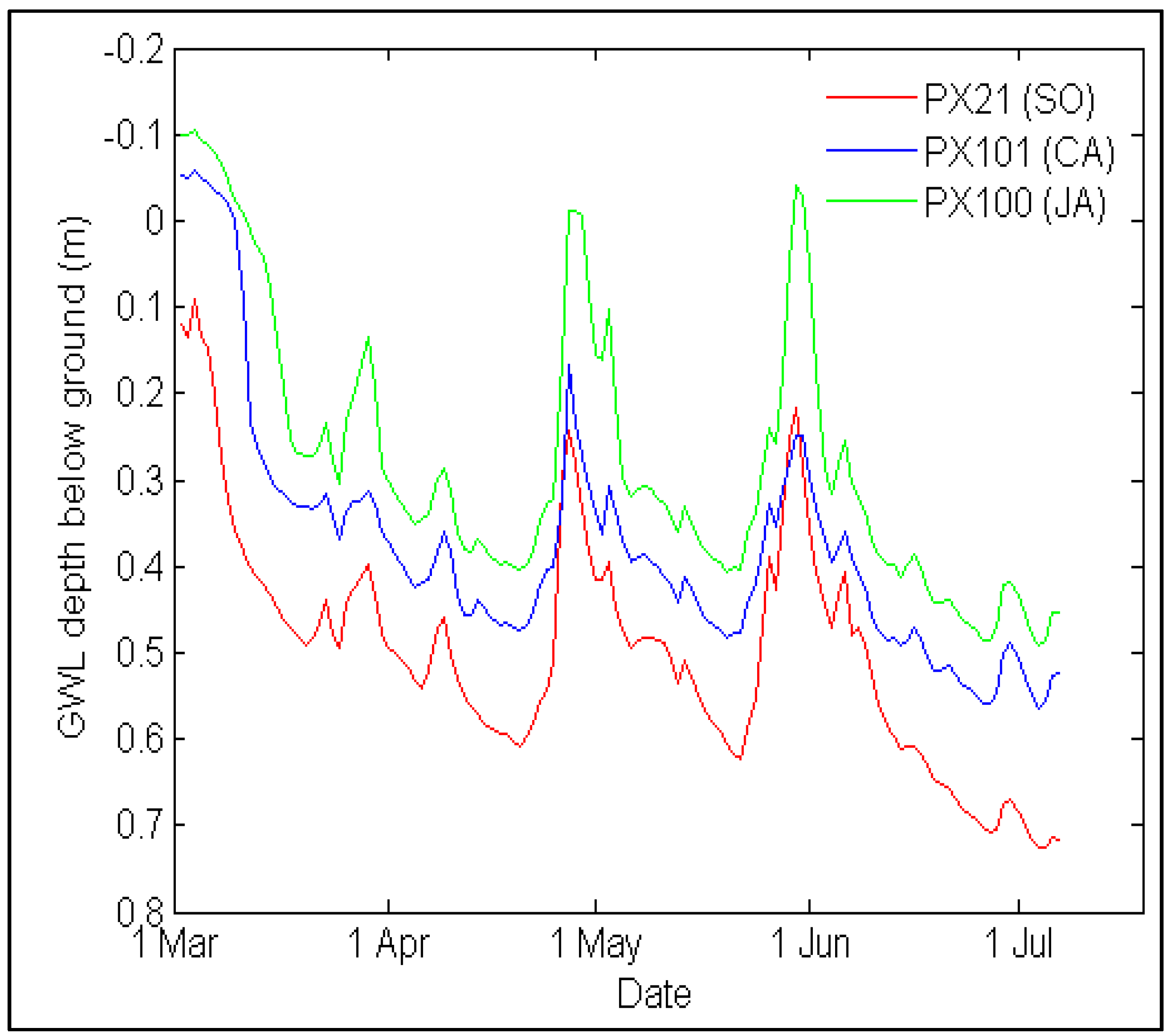
3.6. Groundwater Level Data Acquisition
4. Results
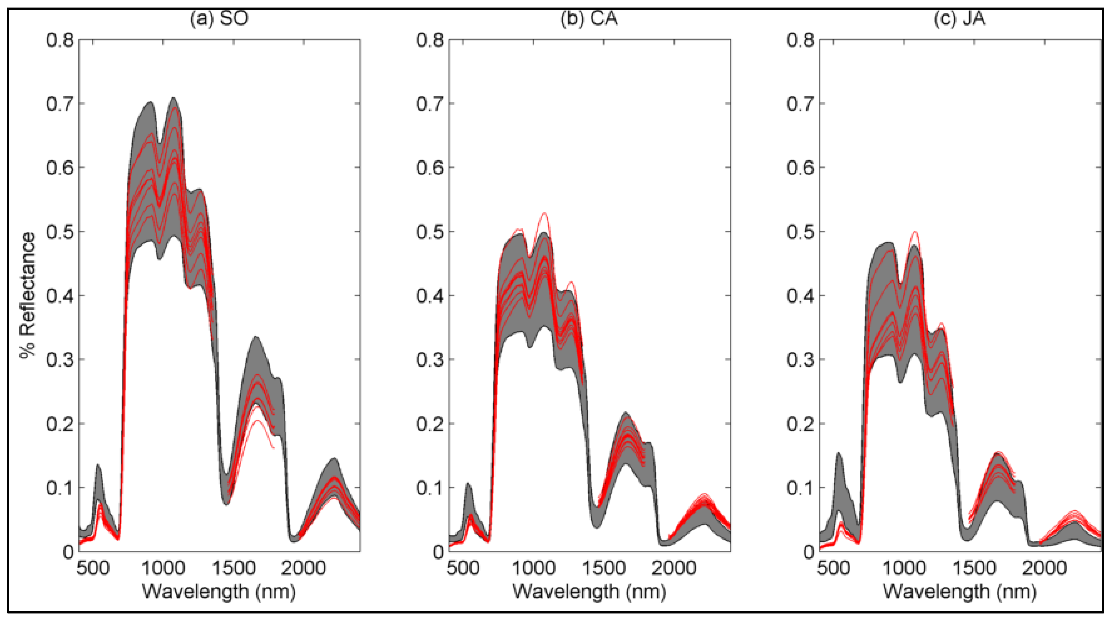
4.1. Spectral Variations
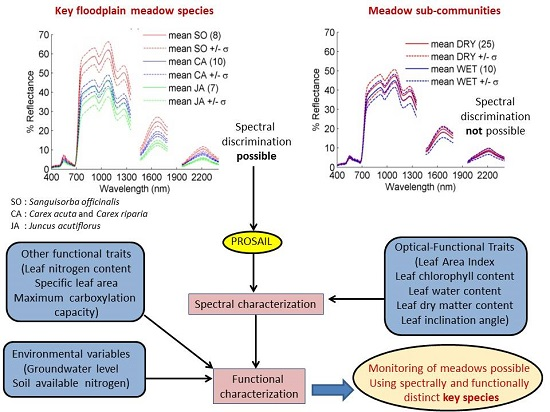
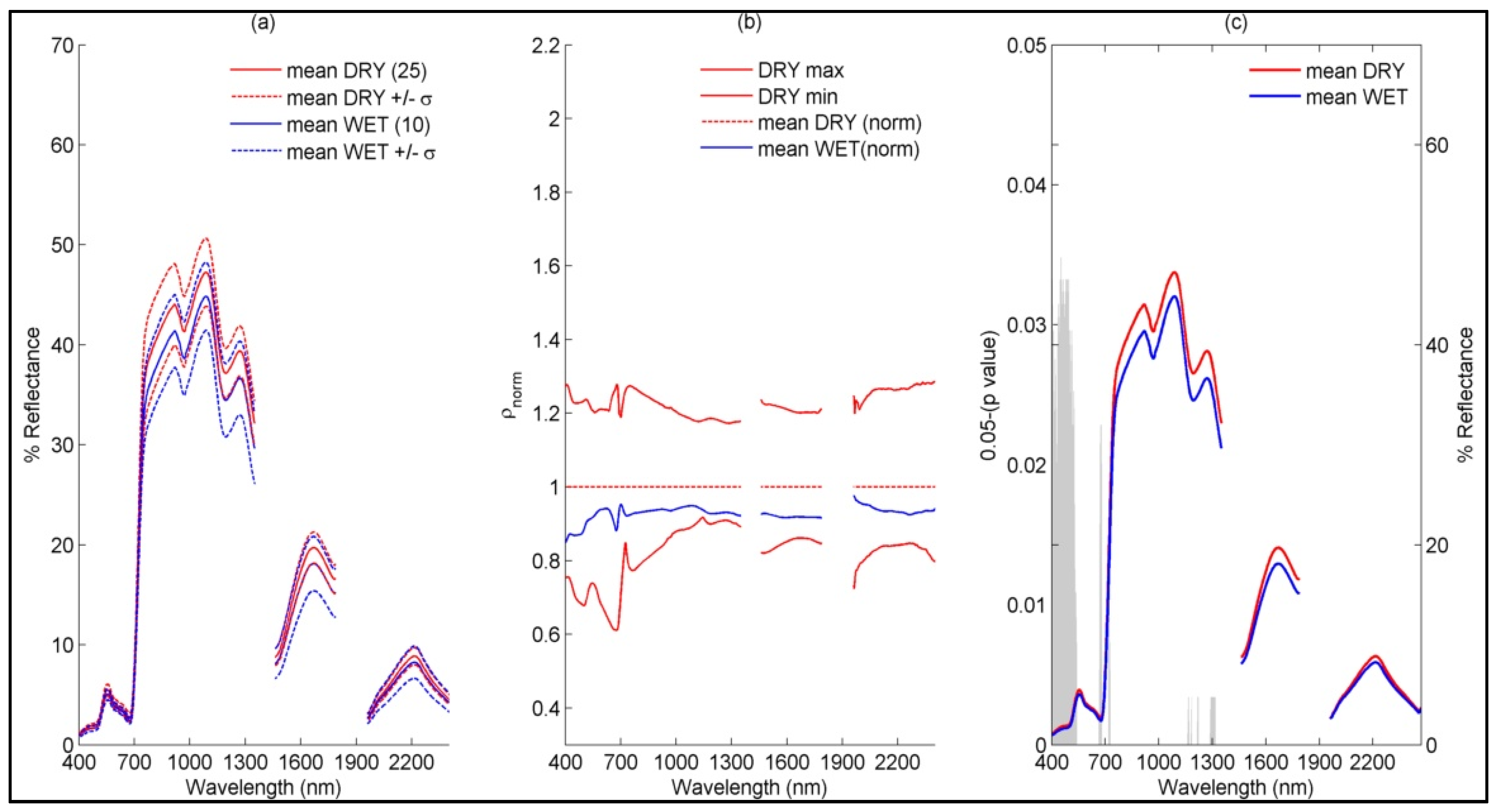
4.1.1. Sub-Community Based Spectral Discrimination

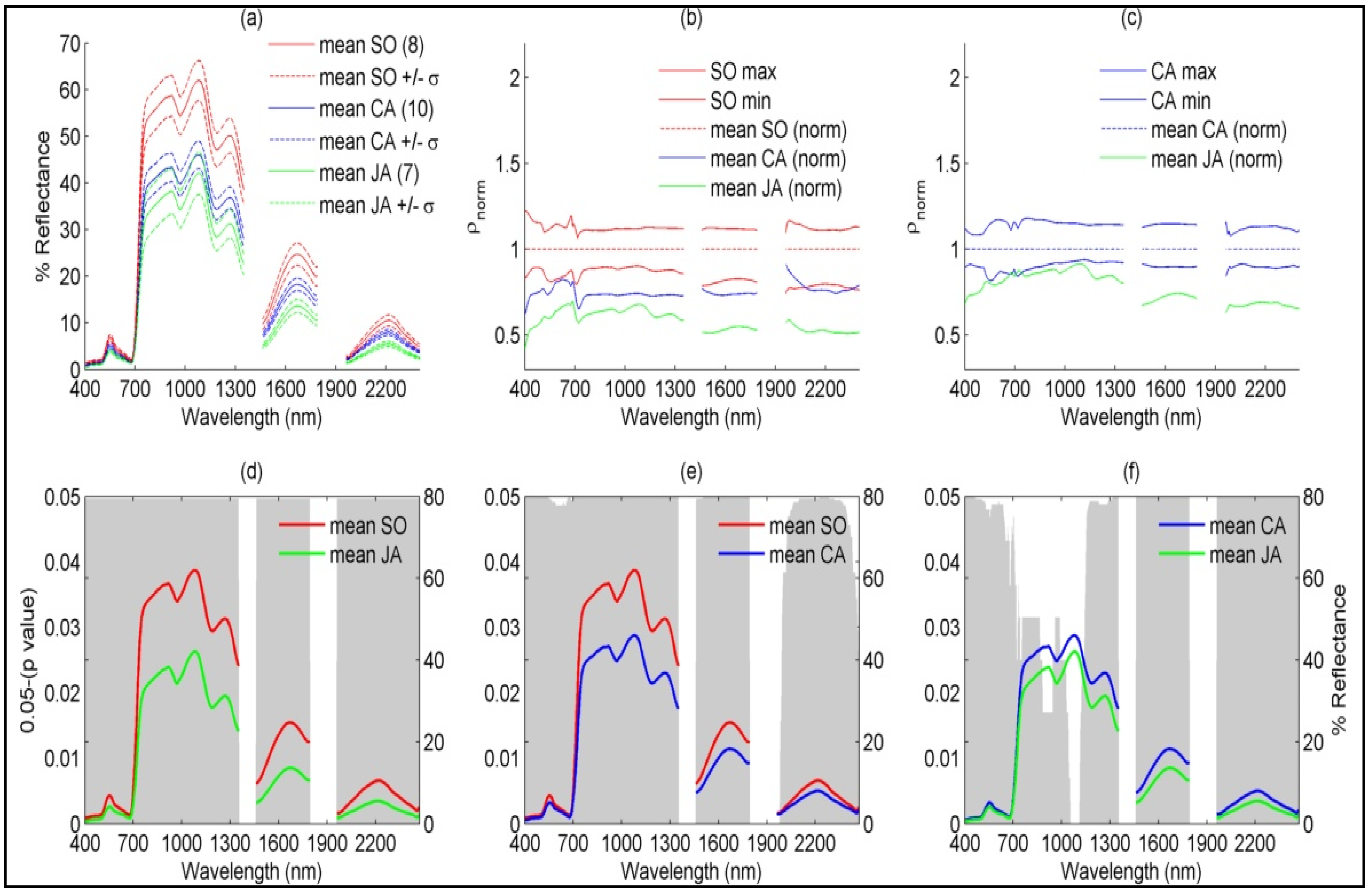
4.1.2. Species-Based

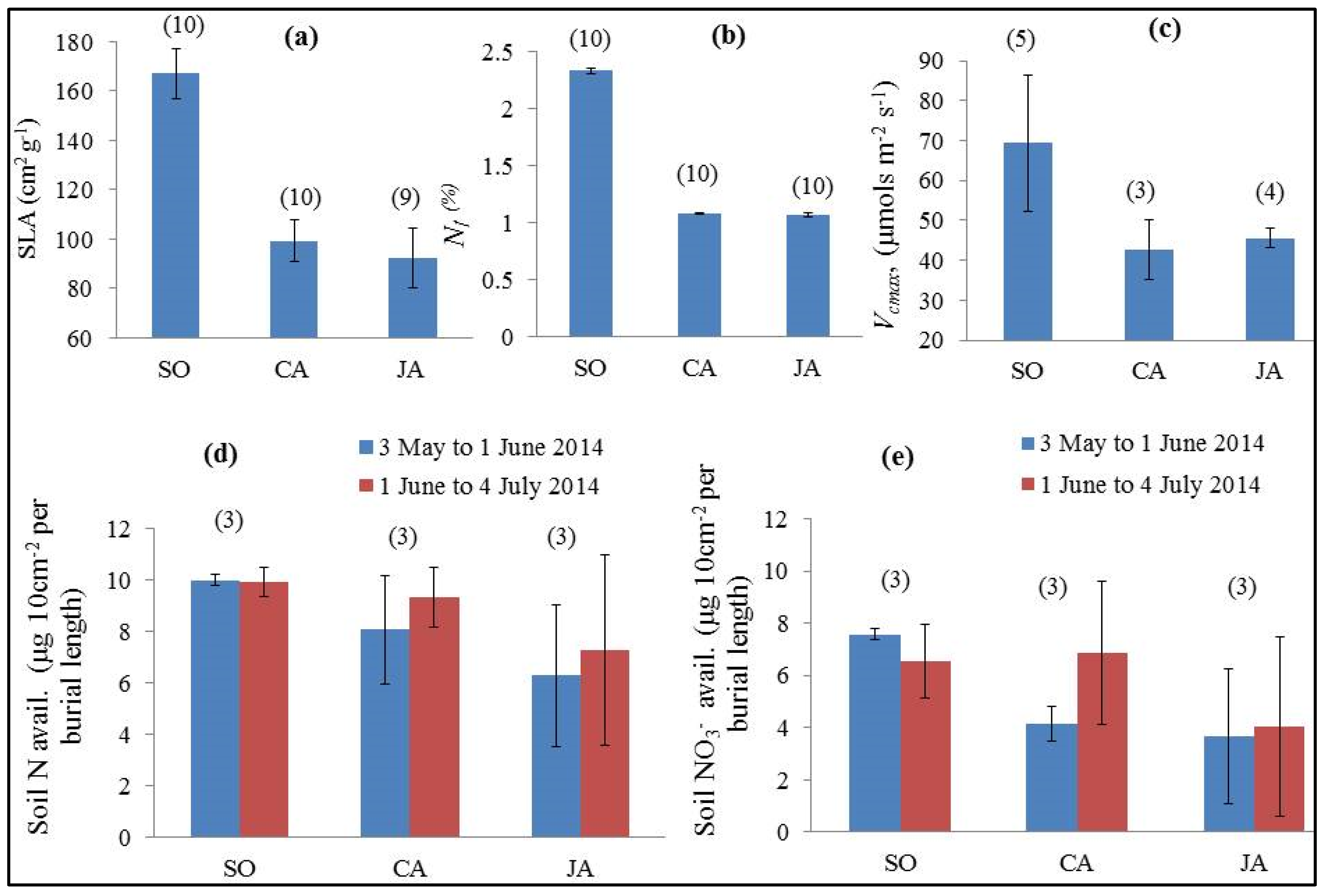
4.2. Vegetation Biophysical and Functional Differences

| Parameter (unit) | Average (Standard Deviation) | p-Value | Significantly Different Pairs | ||
|---|---|---|---|---|---|
| SO | CA | JA | |||
| LAI (m2·m−2) 7 May 2014 | 5.65 (1.55) | 4.24 (0.93) | 3.34 (0.93) | 0.002 | SO–CA; SO–JA |
| LAI (m2·m−2) 1 June 2014 | 7.31 (1.65) | 5.99 (0.84) | 4.19 (0.98) | <0.001 | SO–JA; SO–CA ;JA–CA |
| LAI (m2·m−2) 13 June 2014 | 7.88 (1.52) | 6.69 (1.03) | 5.88 (0.94) | 0.001 | SO–JA; SO–CA |
| Lcc (µg·cm−2) (13 June 2014-for all leaf parameters) | 32.59 (2.26) | 31.54 (3.94) | 23.54 (5.12) | <0.001 | SO–JA; JA–CA |
| Ldmc (g·cm−2) | 0.006 (0.0004) | 0.010 (0.0008) | 0.011 (0.001) | <0.001 | SO–JA; SO–CA; JA–CA |
| Lwc (cm) | 0.010 (0.001) | 0.020 (0.002) | 0.030 (0.003) | <0.001 | SO–JA; SO–CA; JA–CA |
| SLA (cm2·g−1) | 167.01 (10.30) | 99.34 (8.31) | 94.99 (9.31) | <0.001 | SO–JA; SO–CA; JA–CA |
| Vcmax (µg·cm−2·s−1) | 64.51 (16.53) | 39.81 (6.53) | 42.93 (2.20) | <0.001 | SO–JA; SO–CA |
| Nl (%) | 2.33 (0.03) | 1.08 (0.01) | 1.07 (0.02) | <0.001 | SO–JA; SO–CA |
| Nl:Cl | 0.054 (0.0007) | 0.024 (0.0005) | 0.024 (0.0003) | <0.001 | SO–JA; SO–CA |
| (May–June 2014) | 2.39 (0.04) | 3.90 (1.45) | 2.63 (0.20) | 0.142 | none |
| (May–June 2014) | 7.58 (0.23) | 4.15 (0.66) | 3.66 (2.56) | 0.040 | SO–JA; SO–CA |
| (June–July 2014) | 3.35 (0.91) | 3.70 (0.06) | 2.86 (0.43) | 0.403 | none |
| (June–July 2014) | 6.55 (1.39) | 6.86 (2.74) | 4.05 (3.44) | 0.420 | none |
| GWL | Time series data | <0.001 | SO–JA; SO–CA; JA–CA | ||

4.3. Radiative Transfer Model Simulations


4.4. Soil Nitrogen Availability and Groundwater Level Variations

5. Discussion
5.1. Explaining Spectral Variability of Meadow Vegetation
5.2. Functional Differences in SO, CA and JA and Optical Parameters as Functional Traits
5.3. Functional Traits as Ecosystem Monitoring Tool
6. Conclusions
Acknowledgments
Author Contributions
Conflicts of Interest
References
- Gowing, D.J.G.; Tallowin, J.; Dise, N.; Goodyear, J.; Dodd, M.; Lodge, R. A Review of the Ecology, Hydrology and Nutrient Dynamics of Floodplain Meadows in England; English Nature: Peterborough, UK, 2002. [Google Scholar]
- Wheeler, B.D.; Gowing, D.J.G.; Shaw, S.C.; Mountford, J.O.; Money, R.P. Ecohydrological guidelines for lowland wetland plant communities; Brooks, A.E., Jose, P.V., Whiteman, M.I., Eds.; Environmental Agency (Anglian Region): Peterborough, UK, 2004. [Google Scholar]
- Posthumus, H.; Rouquette, J.R.; Morris, J.; Gowing, D.J. G.; Hess, T.M. A framework for the assessment of ecosystem goods and services; A case study on lowland floodplains in England. Ecol. Econ. 2010, 69, 1510–1523. [Google Scholar] [CrossRef]
- Tockner, K.; Stanford, J.A. Riverine flood plains: Present state and future trends. Environ. Conserv. 2002, 29, 308–330. [Google Scholar] [CrossRef]
- Van Diggelen, R.; Middleton, B.; Bakker, J.; Grootjans, A.; Wassen, M. Fens and floodplains of the temperate zone: Present status, threats, conservation and restoration. Appl. Veg. Sci. 2006, 9, 157–162. [Google Scholar] [CrossRef]
- Wallace, J.; Verhoef, A. Modelling interactions in mixed-plant communties: Light, water and carbon dioxide. In Leaf Development and Canopy Growth; Marshall, B., Roberts, J.A., Eds.; Sheffield Academic Press: Sheffield, UK, 2000; pp. 204–250. [Google Scholar]
- Jones, H.G.; Vaughan, R.A. Remote Sensing of Vegetation: Principles, Techniques and Applications; Oxford University Press: Oxford, UK, 2010. [Google Scholar]
- Kerr, J.T.; Ostrovsky, M. From space to species: Ecological applications for remote sensing. Trends Ecol. Evol. 2003, 18, 299–305. [Google Scholar] [CrossRef]
- Thomson, A.G.; Fuller, R.M.; Yates, M.G.; Brown, S.L.; Cox, R.; Wadsworth, R.A. The use of airborne remote sensing for extensive mapping of intertidal sediments and saltmarshes in eastern England. Int. J. Remote Sens. 2003, 24, 2717–2737. [Google Scholar] [CrossRef]
- Xie, Y.; Sha, Z.; Yu, M. Remote sensing imagery in vegetation mapping: A review. J. Plant Ecol. 2008, 1, 9–23. [Google Scholar] [CrossRef]
- Oldeland, J.; Wesuls, D.; Rocchini, D.; Schmidt, M.; Jürgens, N. Does using species abundance data improve estimates of species diversity from remotely sensed spectral heterogeneity? Ecol. Indic. 2010, 10, 390–396. [Google Scholar] [CrossRef]
- Rocchini, D. Effects of spatial and spectral resolution in estimating ecosystem alpha diversity by satellite imagery. Remote Sens. Environ. 2007, 111, 423–434. [Google Scholar] [CrossRef]
- Baret, F.; Fourty, T. Estimation of leaf water content and specific leaf weight from reflectance and transmittance measurements. Agronomie 1997, 17, 455–464. [Google Scholar] [CrossRef]
- Clevers, J.G.P.W.; Gitelson, A.A. Remote estimation of crop and grass chlorophyll and nitrogen content using red-edge bands on Sentinel-2 and -3. Int. J. Appl. Earth Obs. Geoinf. 2013, 23, 344–351. [Google Scholar] [CrossRef]
- Laurent, V.C.E.; Verhoef, W.; Clevers, J.G.P.W.; Schaepman, M.E. Estimating forest variables from top-of-atmosphere radiance satellite measurements using coupled radiative transfer models. Remote Sens. Environ. 2011, 115, 1043–1052. [Google Scholar] [CrossRef]
- Zheng, G.; Moskal, L.M. Retrieving leaf area index (LAI) using remote sensing: Theories, methods and sensors. Sensors 2009, 9, 2719–2745. [Google Scholar] [CrossRef] [PubMed]
- Marshall, M.; Thenkabail, P. Biomass modeling of four leading world crops using hyperspectral narrowbands in support of HyspIRI mission. Photogramm. Eng. Remote Sens. 2014, 80, 757–772. [Google Scholar] [CrossRef]
- Boegh, E.; Thorsen, M.; Butts, M.B.; Hansen, S.; Christiansen, J.S.; Abrahamsen, P.; Hasager, C.B.; Jensen, N.O.; van der Keur, P.; Refsgaard, J.C.; et al. Incorporating remote sensing data in physically based distributed agro-hydrological modelling. J. Hydrol. 2004, 287, 279–299. [Google Scholar] [CrossRef]
- Dorigo, W.A.; Zurita-Milla, R.; de Wit, A.J.W.; Brazile, J.; Singh, R.; Schaepman, M.E. A review on reflective remote sensing and data assimilation techniques for enhanced agroecosystem modeling. Int. J. Appl. Earth Obs. Geoinf. 2007, 9, 165–193. [Google Scholar] [CrossRef]
- Alfieri, J.G.; Xiao, X.; Niyogi, D.; Pielke Sr, R.A.; Chen, F.; LeMone, M.A. Satellite-based modeling of transpiration from the grasslands in the Southern Great Plains, USA. Glob. Planet. Change 2009, 67, 78–86. [Google Scholar] [CrossRef]
- MacBean, N.; Maignan, F.; Peylin, P.; Bacour, C.; Bréon, F.-M.; Ciais, P. Using satellite data to improve the leaf phenology of a global terrestrial biosphere model. Biogeosciences Discuss. 2015, 12, 13311–13373. [Google Scholar] [CrossRef]
- Ustin, S.L.; DiPietro, D.; Olmstead, K.; Underwood, E.; Scheer, G.J. Hyperspectral remote sensing for invasive species detection and mapping. IGARSS 2002, 3, 1658–1660. [Google Scholar]
- Cho, M.A.; Sobhan, I.; Skidmore, A.K.; Leeuw, J. de Discriminating species using hyperspectral indices at leaf and canopy scales. Remote Sens. Spat. Inf. Sci. 2008, 37, 369–376. [Google Scholar]
- Goetz, A.F.H. Three decades of hyperspectral remote sensing of the Earth: A personal view. Remote Sens. Environ. 2009, 113, S5–S16. [Google Scholar] [CrossRef]
- Asner, G.P.; Martin, R.E.; Carranza-Jiménez, L.; Sinca, F.; Tupayachi, R.; Anderson, C.B.; Martinez, P. Functional and biological diversity of foliar spectra in tree canopies throughout the Andes to Amazon region. New Phytol. 2014, 204, 127–139. [Google Scholar] [CrossRef] [PubMed]
- Marshall, M.; Thenkabail, P. Advantage of hyperspectral EO-1 Hyperion over multispectral IKONOS, GeoEye-1, WorldView-2, Landsat ETM+, and MODIS vegetation indices in crop biomass estimation. ISPRS J. Photogramm. Remote Sens. 2015, 108, 205–218. [Google Scholar] [CrossRef]
- Thenkabail, P.S.; Lyon, J.G.; Huete, A. Hyperspectral Remote Sensing of Vegetation; CRC Press-Taylor and Francis group: Boca Raton, FL, USA, London, UK, New York, NY, USA, 2011. [Google Scholar]
- Gamon, J.A. Tropical remote sensing—Opportunities and challenges. In Hyperspectral Remote Sening of Tropical and Subtropical Forests; Kalacska, M., Sanchez-Azofiefa, G.A., Eds.; CRC Press Taylor and Francis Group: Boca Raton, FL, USA, 2008; pp. 207–304. [Google Scholar]
- Ustin, S.L.; Gamon, J.A. Remote sensing of plant functional types. New Phytol. 2010, 186, 795–816. [Google Scholar] [CrossRef] [PubMed]
- Ollinger, S.V. Sources of variability in canopy reflectance and the convergent properties of plants. New Phytol. 2011, 189, 375–394. [Google Scholar] [CrossRef] [PubMed]
- Homolová, L.; Malenovský, Z.; Clevers, J.G.P.W.; García-Santos, G.; Schaepman, M.E. Review of optical-based remote sensing for plant trait mapping. Ecol. Complex. 2013, 15, 1–16. [Google Scholar] [CrossRef]
- Artigas, F.J.; Yang, J.S. Hyperspectral remote sensing of marsh species and plant vigour gradient in the New Jersey Meadowlands. Int. J. Remote Sens. 2005, 26, 5209–5220. [Google Scholar] [CrossRef]
- Kahmen, S.; Poschlod, P. Effects of grassland management on plant functional trait composition. Agric. Ecosyst. Environ. 2008, 128, 137–145. [Google Scholar] [CrossRef]
- Rusch, G.M.; Skarpe, C.; Halley, D.J. Plant traits link hypothesis about resource-use and response to herbivory. Basic Appl. Ecol. 2009, 10, 466–474. [Google Scholar] [CrossRef]
- Schellberg, J.; Pontes, L.D.S. Plant functional traits and nutrient gradients on grassland. Grass Forage Sci. 2012, 67, 305–319. [Google Scholar] [CrossRef]
- Asner, G.P. Biophysical and biochemical sources of variability in canopy reflectance. Remote Sens. Environ. 1997, 64, 234–253. [Google Scholar] [CrossRef]
- Jacquemoud, S.; Verhoef, W.; Baret, F.; Bacour, C.; Zarco-Tejada, P.J.; Asner, G.P.; François, C.; Ustin, S.L. PROSPECT + SAIL models: A review of use for vegetation characterization. Remote Sens. Environ. 2009, 113, S56–S66. [Google Scholar] [CrossRef]
- Roelofsen, H.D.; van Bodegom, P.M.; Kooistra, L.; Witte, J.P.M. Trait estimation in herbaceous plant assemblages from in situ canopy spectra. Remote Sens. 2013, 5, 6323–6345. [Google Scholar] [CrossRef]
- Roelofsen, H.D.; van Bodegom, P.M.; Kooistra, L.; Witte, J.P.M. Predicting leaf traits of herbaceous species from their spectral characteristics. Ecol. Evol. 2014, 4, 706–719. [Google Scholar] [CrossRef] [PubMed]
- Möckel, T.; Dalmayne, J.; Prentice, H.; Eklundh, L.; Purschke, O.; Schmidtlein, S.; Hall, K. Classification of grassland successional stages using airborne hyperspectral imagery. Remote Sens. 2014, 6, 7732–7761. [Google Scholar] [CrossRef]
- Schmidt, K.S.; Skidmore, A.K. Spectral discrimination of vegetation types in a coastal wetland. Remote Sens. Environ. 2003, 85, 92–108. [Google Scholar] [CrossRef]
- Sha, Z.; Bai, Y.; Xie, Y.; Yu, M.; Zhang, L. Using a hybrid fuzzy classifier (HFC) to map typical grassland vegetation in Xilin River Basin, Inner Mongolia, China. Int. J. Remote Sens. 2008, 29, 2317–2337. [Google Scholar] [CrossRef]
- Beeri, O.; Phillips, R.; Hendrickson, J.; Frank, A.B.; Kronberg, S. Estimating forage quantity and quality using aerial hyperspectral imagery for northern mixed-grass prairie. Remote Sens. Environ. 2007, 110, 216–225. [Google Scholar] [CrossRef]
- Li, J.; Liang, T.; Chen, Q. Estimating grassland yields using remote sensing and GIS technologies in China. New Zeal. J. Agric. Res. 1998, 41, 31–38. [Google Scholar]
- Darvishzadeh, R.; Skidmore, A.; Schlerf, M.; Atzberger, C. Inversion of a radiative transfer model for estimating vegetation LAI and chlorophyll in a heterogeneous grassland. Remote Sens. Environ. 2008, 112, 2592–2604. [Google Scholar] [CrossRef]
- Cayrol, P.; Chehbouni, A.; Kergoat, L.; Dedieu, G.; Mordelet, P.; Nouvellon, Y. Grassland modeling and monitoring with SPOT-4 VEGETATION instrument during the 1997–1999 SALSA experiment. Agric. For. Meteorol. 2000, 105, 91–115. [Google Scholar] [CrossRef]
- Adam, E.; Mutanga, O.; Rugege, D. Multispectral and hyperspectral remote sensing for identification and mapping of wetland vegetation: A review. Wetl. Ecol. Manag. 2010, 18, 281–296. [Google Scholar] [CrossRef]
- Svoray, T.; Perevolotsky, A.; Atkinson, P.M. Ecological sustainability in rangelands: the contribution of remote sensing. Int. J. Remote Sens. 2013, 34, 6216–6242. [Google Scholar] [CrossRef]
- Rodwell, J.S. British Plant Communities. Volume 3. Grasslands and Montane Communities; Cambridge University Press: Cambridge, UK, 1992. [Google Scholar]
- Passarge, H. Pflanzengesellschaften des nordostdeutschen Flachlandes, Pflanzensoziologie, 13th ed.; Gustav Fischer Verlag: Jena, Germany, 1964. [Google Scholar]
- Araya, Y.; Silvertown, J. A fundamental, ecohydrological basis for niche segregation in plant communities. New Phytol. 2010, 189, 253–258. [Google Scholar] [CrossRef] [PubMed]
- Macdonald, D.M.J.; Dixon, A.; Newell, A.; Hallaways, A. Groundwater flooding within an urbanised flood plain. J. Flood Risk Manag. 2012, 5, 68–80. [Google Scholar] [CrossRef]
- Minasny, B.; McBratney, A.B. A conditioned Latin hypercube method for sampling in the presence of ancillary information. Comput. Geosci. 2006, 32, 1378–1388. [Google Scholar] [CrossRef]
- Wallace, H.L.; Prosser, M.V.; Dodd, M.E.; Sargent, E.; Gowing, D.J.G. Botanical Monitoring (2006–2008) and NVC Survey (2008) of the Oxford Floodplain Meadows; The Floodplain Meadows Partnership: Oxford, UK, 2008. [Google Scholar]
- Hill, M.O.; Mountford, J.O.; Roy, D.B.; Bunce, R.G.H. Ellenberg’s Indicator Values for British Plants; Institute of Terrestrial Ecology: Huntington, UK, 1999. [Google Scholar]
- Cochrane, M.A. Using vegetation reflectance variability for species level classification of hyperspectral data. Int. J. Remote Sens. 2000, 21, 2075–2087. [Google Scholar] [CrossRef]
- Clark, M.L.; Roberts, D.A.; Clark, D.B. Hyperspectral discrimination of tropical rain forest tree species at leaf to crown scales. Remote Sens. Environ. 2005, 96, 375–398. [Google Scholar] [CrossRef]
- Manevski, K.; Manakos, I.; Petropoulos, G.P.; Kalaitzidis, C. Discrimination of common Mediterranean plant species using field spectroradiometry. Int. J. Appl. Earth Obs. Geoinf. 2011, 13, 922–933. [Google Scholar] [CrossRef]
- Inskeep, W.P.; Bloom, P.R. Extinction coefficients of chlorophyll a and b in n,n-dimethylformamide and 80% acetone. Plant Physiol. 1985, 77, 483–485. [Google Scholar] [CrossRef] [PubMed]
- Zhang, J.; Han, C.; Liu, Z. Absorption spectrum estimating rice chlorophyll Concentration: Preliminary investidation. J. Plant Breed. Crop Sci. 2008, 5, 223–229. [Google Scholar] [CrossRef]
- Long, S.P.; Bernacchi, C.J. Gas exchange measurements, what can they tell us about the underlying limitations to photosynthesis? Procedures and sources of error. J. Exp. Bot. 2003, 54, 2393–2401. [Google Scholar] [CrossRef] [PubMed]
- Berry, J.A.; van der Tol, C.; Kornfeld, A. A testbed for model development. AGU Fall Meet. Abstr. 2014, 1, 41. [Google Scholar]
- Verhoef, W. Light scattering by leaf layers with application to canopy reflectance modeling: The SAIL model. Remote Sens. Environ. 1984, 16, 125–141. [Google Scholar] [CrossRef]
- Jacquemoud, S.; Baret, F. PROSPECT: A model of leaf optical properties spectra. Remote Sens. Environ. 1990, 34, 75–91. [Google Scholar] [CrossRef]
- Weiss, M.; Baret, F.; Myneni, R.B.; Pragnere, A.; Knyazikhin, Y. Investigation of a model inversion technique to estimate canopy biophysical variables from spectral and directional reflectance data. Agronomie 2000, 20, 3–22. [Google Scholar] [CrossRef]
- Fourty, T.; Baret, F.; Jacquemoud, S.; Schmuck, G.; Verdebout, J. Leaf optical properties with explicit description of its biochemical composition: Direct and inverse problems. Remote Sens. Environ. 1996, 56, 104–117. [Google Scholar] [CrossRef]
- Bowyer, P.; Danson, F.M. Sensitivity of spectral reflectance to variation in live fuel moisture content at leaf and canopy level. Remote Sens. Environ. 2004, 92, 297–308. [Google Scholar] [CrossRef]
- Asner, G.P.; Jones, M.O.; Martin, R.E.; Knapp, D.E.; Hughes, R.F. Remote sensing of native and invasive species in Hawaiian forests. Remote Sens. Environ. 2008, 112, 1912–1926. [Google Scholar] [CrossRef]
- Adam, E.; Mutanga, O. Spectral discrimination of papyrus vegetation (Cyperus papyrus L.) in swamp wetlands using field spectrometry. ISPRS J. Photogramm. Remote Sens. 2009, 64, 612–620. [Google Scholar] [CrossRef]
- Wang, L.; Qu, J.J.; Hao, X.; Hunt, E.R. Estimating dry matter content from spectral reflectance for green leaves of different species. Int. J. Remote Sens. 2011, 32, 7097–7109. [Google Scholar] [CrossRef]
- Ansquer, P.; Duru, M.; Theau, J.P.; Cruz, P. Convergence in plant traits between species within grassland communities simplifies their monitoring. Ecol. Indic. 2009, 9, 1020–1029. [Google Scholar] [CrossRef]
- Wilson, P.J.; Thompson, K.; Hodgson, J.G. Specific leaf area and dry leaf matter content as alternative predictors of plant strategies. New Phytol. 1999, 143, 155–162. [Google Scholar] [CrossRef]
- Reich, P.B.; Ellsworth, D.S.; Walters, M.B. Leaf structure (specific leaf area) modulates photosynthesis-nitrogen relations: Evidence from within and across species and functional groups. Funct. Ecol. 1998, 12, 948–958. [Google Scholar] [CrossRef]
- Kattge, J.; Knorr, W.; Raddatz, T.; Wirth, C. Quantifying photosynthetic capacity and its relationship to leaf nitrogen content for global-scale terrestrial biosphere models. Glob. Chang. Biol. 2009, 15, 976–991. [Google Scholar] [CrossRef]
- Wohlfahrt, G.; Bahn, M.; Haubner, E.; Horak, I.; Michaeler, W.; Rottmar, K.; Tappeiner, U.; Cernusca, A. Inter-specific variation of the biochemical limitation to photosynthesis and related leaf traits of 30 species from mountain grassland ecosystems under different land use. Plant, Cell Environ. 1999, 22, 1281–1296. [Google Scholar] [CrossRef]
- Craine, J.M.; Tilman, D.; Wedin, D.; Reich, P.; Tjoelker, M.; Knops, J. Functional traits, productivity and effects on nitrogen cycling of 33 grassland species. Funct. Ecol. 2002, 16, 563–574. [Google Scholar] [CrossRef]
- Sheremetiev, S.N. Meadow Vegetation at the Soil Moisture Gradient; KMK: Moscow, Russia, 2005. [Google Scholar]
- Grime, J.P. Evidence for the existence of three primary strategies in plants and its relevance to ecological and evolutionary theory. Am. Nat. 1977, 111, 1169–1194. [Google Scholar] [CrossRef]
- Schmidtlein, S.; Feilhauer, H.; Bruelheide, H. Mapping plant strategy types using remote sensing. J. Veg. Sci. 2012, 23, 395–405. [Google Scholar] [CrossRef]
- Chavana-Bryant, C.; Malhi, Y.; Jin, W.; Asner, G.; Athanasios, A.; Brian, E.; Scott, S.; Christopher, D.; Roberta, M.; France, G. Leaf aging of Amazonian canopy trees revealed by spectral and physiochemical measurements. New Phytol. 2016. In press. [Google Scholar]
© 2016 by the authors; licensee MDPI, Basel, Switzerland. This article is an open access article distributed under the terms and conditions of the Creative Commons by Attribution (CC-BY) license (http://creativecommons.org/licenses/by/4.0/).
Share and Cite
Punalekar, S.; Verhoef, A.; Tatarenko, I.V.; Van der Tol, C.; Macdonald, D.M.J.; Marchant, B.; Gerard, F.; White, K.; Gowing, D. Characterization of a Highly Biodiverse Floodplain Meadow Using Hyperspectral Remote Sensing within a Plant Functional Trait Framework. Remote Sens. 2016, 8, 112. https://doi.org/10.3390/rs8020112
Punalekar S, Verhoef A, Tatarenko IV, Van der Tol C, Macdonald DMJ, Marchant B, Gerard F, White K, Gowing D. Characterization of a Highly Biodiverse Floodplain Meadow Using Hyperspectral Remote Sensing within a Plant Functional Trait Framework. Remote Sensing. 2016; 8(2):112. https://doi.org/10.3390/rs8020112
Chicago/Turabian StylePunalekar, Suvarna, Anne Verhoef, Irina V. Tatarenko, Christiaan Van der Tol, David M. J. Macdonald, Benjamin Marchant, France Gerard, Kevin White, and David Gowing. 2016. "Characterization of a Highly Biodiverse Floodplain Meadow Using Hyperspectral Remote Sensing within a Plant Functional Trait Framework" Remote Sensing 8, no. 2: 112. https://doi.org/10.3390/rs8020112
APA StylePunalekar, S., Verhoef, A., Tatarenko, I. V., Van der Tol, C., Macdonald, D. M. J., Marchant, B., Gerard, F., White, K., & Gowing, D. (2016). Characterization of a Highly Biodiverse Floodplain Meadow Using Hyperspectral Remote Sensing within a Plant Functional Trait Framework. Remote Sensing, 8(2), 112. https://doi.org/10.3390/rs8020112