Integration of Aerial Thermal Imagery, LiDAR Data and Ground Surveys for Surface Temperature Mapping in Urban Environments

Abstract

A single-band surface temperature retrieval method is proposed, aiming at achieving a better accuracy by exploiting the integration of aerial thermal images with LiDAR data and ground surveys. LiDAR data allow the generation of a high resolution digital surface model and a detailed modeling of the Sky-View Factor (SVF). Ground surveys of surface temperature and emissivity, instead, are used to estimate the atmospheric parameters involved in the model (through a bounded least square adjustment) and for a first assessment of the accuracy of the results. The RMS of the difference between the surface temperatures computed from the model and measured on the check sites ranges between 0.8 °C and 1.0 °C, depending on the algorithm used to calculate the SVF. Results are in general better than the ones obtained without considering SVF and prove the effectiveness of the integration of different data sources. The proposed approach has the advantage of avoiding the modeling of the atmosphere conditions, which is often difficult to achieve with the desired accuracy; on the other hand, it is highly dependent on the accuracy of the data measured on the ground.

1. Introduction

The increasing attention for energy-saving strategies and for the reduction of carbon emissions has been renewing the interest for the applications of thermography in urban environments. In fact, in European countries, the building sector accounts for more than one third of the total energy use, providing huge potential for energy savings [1]. Thermography has proven to be an important tool for analyzing the thermal characteristics of the materials lying on the ground, as well as many processes related to the exchange of heat between surfaces.

A wide range of military, civil, industrial and scientific applications has been described in the literature [2,3]. In particular, remotely-sensed imagery in the thermal infrared is able to provide a synoptic and time-synchronized view of the investigated landscape, allowing the generation of coherent maps of surface temperature [4,5]. Airborne sensors are also able to acquire data at high geometrical resolution over very large areas, so they can be applied for the evaluation of the energetic performance of buildings at an urban scale [6,7,8].

The present work focuses on a surface temperature retrieval process that exploits images acquired in the thermal band (7–16 microns) by a single channel sensor, installed on an aircraft. Starting from the conclusions by Bitelli et al. [9], this work aims at achieving a better accuracy through the integration of LiDAR data and ground surveys for calibration purposes.

LiDAR data allow the mapping of the Sky-View Factor (SVF), a parameter that influences the radiation exchange between surfaces and the surrounding environment and is neglected in many simplified methods proposed in the literature for practical reasons.

SVF is one of the most relevant parameters in climate modeling and in particular in human-biometeorology, which deals with the effects of weather conditions, climate and air quality on human beings [10]. It has a strong influence on the exchange of heat in complex structures, and thus, it is widely used in urban climatology, where the presence of many structures and obstacles strongly influences the incoming radiation fluxes on each point of the urban texture. For example, in a street canyon, the energy budget is affected by reflections of short-wave radiation, a decrease in outgoing long-wave radiation, an increase in received long-wave radiation that is emitted by the surfaces, which obstruct the sky, and consequently, an altered soil heat flux [11].

For the topics discussed in this paper, SVF influences the amount of both downwelling radiation coming from the sky and radiation coming from the surroundings objects (e.g., other buildings), which are reflected by the target surface in the observing direction, thus altering temperature measurements by an infrared sensor.

SVF computation has been widely investigated [12,13,14], especially in urban areas, where the presence of urban canyons and structures, in general, can strongly influence the energy exchange between surfaces and the atmosphere, modifying microclimate conditions at the ground level. In recent years, several software applications have been developed for the calculation of this parameter, using as input different datasets pertaining to building geometry, the morphology of the investigated area and the presence of other obstacles (like trees).

From a remote sensing perspective, applications that use digital surface models as the main input are particularly promising: in fact, they permit the computation of SVF values even on large areas (up to the entire city), with a regular spacing, using a unique data type that can be obtained from different sources (such as LiDAR surveys, stereographic aerial or satellite imagery, digitalization of contour lines). In addition, generally, they do not strictly need the availability of vectorial datasets containing building footprints and elevations, but can use them as additional data to improve the quality of results. Recently, algorithms for SVF computation [15,16] have been refined so that they can consider not only the position and orientation of obstacles, but also their nature (trees or buildings) and characteristics in terms of shape and transparency.

However, these algorithms were created and tested only at the ground level, because they are focused on the assessment of microclimate conditions on streets, parks, squares and other areas where people usually live and move. It is therefore interesting to test their usability also with roof surfaces, where the assessment of the sky-view factor is necessary for a proper radiometric correction of thermal imagery acquired from an airborne infrared sensor.

Another aspect that has a valuable impact on the final accuracy is the atmospheric correction. An accurate modeling of the atmospheric absorption and emission phenomena would require a detailed description of the physical state of the entire atmosphere column above the investigated area. This means that vertical profiles of atmospheric temperature, pressure and humidity should be collected together with information about the mixing ratio of the main gaseous species, especially those affecting the thermal band (e.g., ozone and carbon dioxide). Unfortunately, these data are often unavailable, and only approximated solutions can be obtained using satellite products (e.g., MODIS) and general-purpose climatic models.

The approach proposed here tries to overcome this limitation by exploiting ground surveys, to be performed concurrently with the aerial thermal imagery acquisition. Data acquired on the ground encompass the temperature, emissivity and sky-view factor of a limited number of surfaces visible from aerial images and can be used to estimate the atmospheric parameters figuring in the radiative transfer equations.

Finally, an accurate temperature estimation requires a proper emissivity assessment. Multi-band methods allow the simultaneous computation of temperature and emissivity [17], but they generally rely on some simplification of Planck’s law, because the problem is ill-posed. In fact, even with multi-spectral sensors with N thermal channels available, the system composed of N radiative transfer equations (one for each channel) remains mathematically unsolvable, because there will always be $N+$ 1 unknowns, corresponding to the N emissivities in each wavelength and the surface temperature [18]. Single-band methods, instead, require a derivation of emissivity from external data, such as NDVI maps [19] or land-cover maps [20], which can be produced also by multispectral or hyperspectral optical imagery.

All of the activities presented here were conducted in the framework of the research project entitled “The Challenge of remote sensing Thermography as an indicator of energy efficiency of buildings” (ChoT), which aims to analyze the potential of aerial thermal imagery to produce large-scale datasets for energetic efficiency analyses and policies in urban environments. The final outcomes of the project are expected to quantify the achievable accuracy in the estimation of surface temperature and its sensitivity to the main variables of the problem.

2. Background Theory

Retrieval of surface temperatures from remote sensing imagery requires a modeling of the sensor system, of the atmospheric conditions at the time of acquisition and a characterization of some surface properties. This section summarizes the theoretical assumptions under the approach proposed in the Methods section. Following the formalism adopted by Bitelli et al. [9], small letters indicate the spectral quantities (which are functions of the wavelength), while the broadband quantities, integrated or averaged over the spectral range to which the thermal camera is sensitive, are designated by capital letters.

A sensor installed on-board an aircraft registers a signal, which is composed of different emitted and reflected contributions (cf. [21,22]). The total spectral radiance reaching the sensor ($l_S$) is given by:

$$l_S=\mathsf{\tau }\mathsf{ϵ}{l}_B+l_u+\mathsf{\rho }\mathsf{\tau }F{l}_d+\mathsf{\rho }\mathsf{\tau }(1-F)l_{sr}$$

(1)

The first contribution is the radiance emitted by the observed surface ($l_B$), which is a function of the surface temperature according to Planck’s law; the quantity is multiplied by the surface emissivity ($\mathsf{ϵ}$), because the surface is not a black-body, and it is attenuated by the atmosphere transmittance ($\mathsf{\tau }$), in order to take into account the atmospheric absorption effect. The second term expresses the upwelling radiance ($l_u$) emitted upward by the atmosphere layer between the surface and the sensor. The last two terms are radiances reflected by the observed surface toward the sensor: $l_d$ is the downwelling radiance from the entire atmosphere column and $l_{sr}$ is the radiance emitted toward the observed surface by the surrounding objects. As a simplification, a Lambertian behavior is assumed for all of the surfaces; thus, surface reflectance ($\mathsf{\rho }=1-\mathsf{ϵ}$) is dependent on the wavelength only and not on the observing geometry. Finally, F is the sky-view factor, the definition of which is discussed later, ranging between zero and one.

Actually, each sensor is sensitive to the incoming radiation in a specific interval of the electromagnetic spectrum. Sensor behavior is described by the relative spectral response function, here designed as s, which varies between zero and one with the wavelength. Spectral quantities are integrated over the broadband.

$$L_S={\displaystyle \frac{{\int }_{\mathsf{\lambda }}{l}_{S}sd\mathsf{\lambda }}{{\int }_{\mathsf{\lambda }}sd\mathsf{\lambda }}}$$

(2)

By substituting Equation (1) in Equation (2) and solving for the $l_B$ term,

$${\int }_{\mathsf{\lambda }}\mathsf{\tau }{l}_{B}sd\mathsf{\lambda }={\displaystyle \frac{{\int }_{\mathsf{\lambda }}{l}_{S}sd\mathsf{\lambda }-{\int }_{\mathsf{\lambda }}{l}_{u}sd\mathsf{\lambda }-PF{\int }_{\mathsf{\lambda }}\mathsf{\tau }{l}_{d}sd\mathsf{\lambda }}{E+P(1-F)}}$$

(3)

where P and E are the broadband reflectance and emissivity, respectively.

To obtain Equation (3), two main simplifications are adopted. Firstly, the radiance emitted by the surrounding objects is assumed to be equal to the one emitted by the target surface ($l_{sr}=l_B$); actually, temperatures of various urban surfaces (roofs, walls, ground) can vary considerably due to differences in the facet-specific energy-balance [23]. A proper modeling of the reflections from surrounding objects requires a detailed 3D model and the evaluation of both surface temperatures and emissivities for all of the facets of the urban texture, but is often neglected due to data unavailability. Although some experiences in the literature tried to solve this complexity in the case of infrared imagery acquired with oblique views over street canyons or single blocks [23,24], these approaches seem hardly feasible when analyzing a whole urban area with aerial imagery. The second assumption is a constant emissivity over the band interval, according to the hypothesis of grey-body behavior. This is mainly suggested by practical considerations about the estimation of the emissivity values for the different materials, because the use of a thermal camera for ground surveys, as discussed later, allows the determination of a single broadband value for each material. Differently from the study by Bitelli et al. [9], however, the sky-view factor is fully considered here for the surface temperature retrieval.

Several formulations of the SVF have been proposed in the literature. According to the definition proposed by Oke [25], a view factor represents the ratio of radiation received by a planar surface to that received from the entire hemispheric radiating environment; thus, the sky-view factor can be expressed as the radiation coming from the visible part of the sky divided by the total radiation from the entire hemisphere [26]:

$$F_L={\displaystyle \frac{\underset{0}{\overset{2\mathsf{\pi }}{\int }}\underset{0}{\overset{\mathsf{\zeta }}{\int }}L(\mathsf{\varphi },\mathsf{\theta })sin\mathsf{\theta }cos\mathsf{\theta }d\mathsf{\theta }d\mathsf{\varphi }}{\underset{0}{\overset{2\mathsf{\pi }}{\int }}\underset{0}{\overset{\mathsf{\pi }/2}{\int }}L(\mathsf{\varphi },\mathsf{\theta })sin\mathsf{\theta }cos\mathsf{\theta }d\mathsf{\theta }d\mathsf{\varphi }}}$$

(4)

where $\mathsf{\varphi }$ and $\mathsf{\theta }$ are the azimuth and polar angular coordinates, respectively, and $\mathsf{\zeta }=\mathsf{\zeta }\left(\mathsf{\varphi }\right)$ is the complementary of the elevation angle from the horizontal plane of the obstacle in a given direction.

Instead, Zakšek et al. [27] defined the SVF as the portion of visible sky in the entire celestial hemisphere centered on the observation point, expressed in terms of solid angle Ω:

$$F_{\mathsf{\Omega }}={\displaystyle \frac{\mathsf{\Omega }}{2\mathsf{\pi }}}={\displaystyle \frac{1}{2\mathsf{\pi }}}{\int }_0^{2\mathsf{\pi }}{\int }_0^{\mathsf{\zeta }}sin\mathsf{\theta }d\mathsf{\theta }d\mathsf{\varphi }$$

(5)

As pointed out by Zhang et al. [28], the two definitions do not coincide even in the case of isotropic radiation (constant L). The first definition comes from the concept of the view factor and accounts for the projection of each element of the observed surface in the plane of the observing surface. Instead, the second definition expresses SVF as the proportion of the sky that is visible from a point to the overall sky dome. With this last meaning, the parameter is also called sky-exposure.

The two definitions lead to numerically different sky-view factors, even if the geometry is the same. For example, considering the theoretical case of a circular basin with a constant elevation angle and an isotropic radiation, the analytical solutions for the observing point located at the center are:

$$\begin{array}{cc}\hfill F_L& ={cos}^2\mathsf{\beta }\hfill \end{array}$$

(6a)

$$\begin{array}{cc}\hfill F_{\mathsf{\Omega }}& =1-sin\mathsf{\beta }\hfill \end{array}$$

(6b)

where $\mathsf{\beta }$ is the elevation angle from the horizontal plane of the obstacle in a given direction.

These formulas for the case of a circular basin can be generalized considering an elevation angle varying with the azimuthal direction [10,15]. This generalization provides a convenient way for the calculation of SVF maps in urban environments.

$$\begin{array}{cc}\hfill F_L& ={\displaystyle \frac{{\displaystyle \sum _{i=0}^n}{cos}^2{\mathsf{\beta }}_i}{n}}\hfill \end{array}$$

(7a)

$$\begin{array}{cc}\hfill F_{\mathsf{\Omega }}& =1-{\displaystyle \frac{{\displaystyle \sum _{i=0}^n}sin{\mathsf{\beta }}_i}{n}}\hfill \end{array}$$

(7b)

where n stands for the number of directions used to estimate the elevation angle of the obstacles.

3. Materials

Even if thermal imagery acquired by an aerial platform is the principal dataset, the proposed approach relies on its integration with (1) LiDAR data to provide SVF maps and (2) ground surveys to estimate the required atmospheric parameters and to control the overall quality of the process.

3.1. Aerial Thermal Images

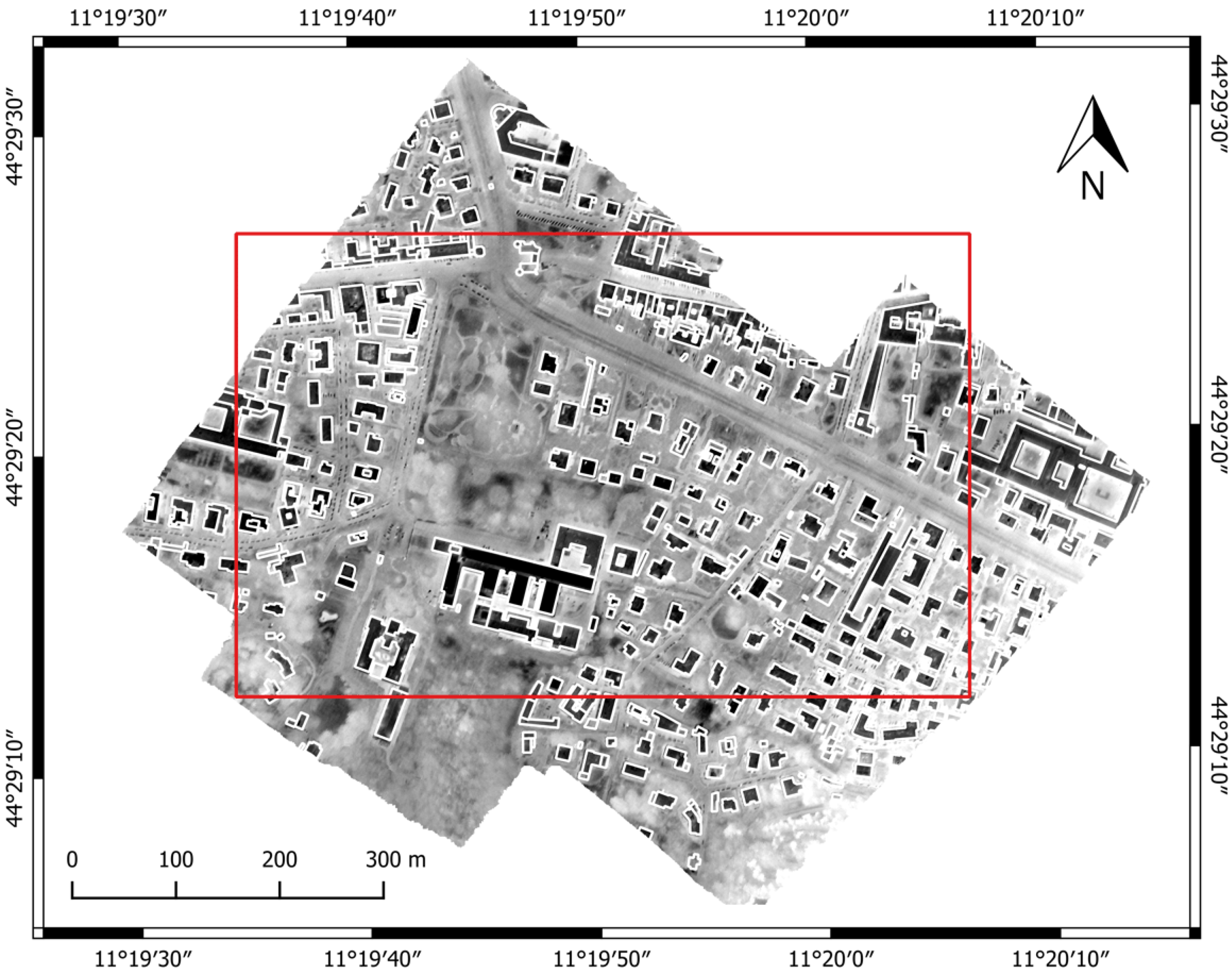
In the framework of the ChoT project, two aerial surveys were carried out on 14 and 15 March 2016 by the National Institute of Oceanography and Experimental Geophysics (OGS) over the urban area of Bologna (Italy). The first flight was performed at night-time, whilst the second during the day, both in conditions of clear sky and light winds. More than 2500 frames were acquired for each flight, over a total area of about 11 km². For the present study, only the data acquired in the night flight were processed, performing all the analyses on a small test area (about 0.44 km²) around the School of Engineering and Architecture of the University of Bologna. The morphology of the area is quite complex, with a ground elevation ranging from 60 to 130 m above the sea level from north to south. The site includes many buildings with variable heights (from 2 to 45 m at the eaves) and some vegetated areas.

The thermal camera used for the acquisition is a NEC TS9260, operating in the long wave infrared (7–16 microns) with a resolution of 640 × 480 pixels and a noise equivalent temperature difference of 0.06 °C. The camera has a quite narrow field of view (21.7 × 16.4 degrees), which helps to reduce the geometric distortion of the lens, but conversely makes it necessary to acquire a big set of thermal scenes to cover a wide area. The flight height was set to approximately 800 m above the ground, in order to obtain a ground sampling distance of about 0.5 m.

The airplane was also equipped with a high precision GPS receiver, an Inertial Measuring Unit (IMU) and a video encoding/decoding device. With this equipment, it is possible to measure with reliable accuracy the position and orientation of the vehicle at each shot, associating with each thermal frame the external orientation parameters necessary for the ortho-mosaicking phase.

Twenty-one frames from three adjacent strips covering the test area were mosaicked and orthorectified (Figure 1) using 60 ground control points, whose coordinates were derived from the technical cartography of the Municipality of Bologna (nominal scale: 1:2000). The processing was carried out using Agisoft Photoscan™, a software based on the “structure from motion” technique [29] that can reconstruct the three-dimensional morphology of a scene when provided with bi-dimensional overlapping frames acquired by terrestrial or aerial digital cameras.

3.2. LiDAR Data

LiDAR data were acquired on 26 January 2009 by Blom CGR S.p.a. The laser scanner used was a Optech ALTM 3033 with a scan width (FOV) of ±11 degrees. Given the operational altitude of 1250 m above the ground level and a distance between the strip axis of 322 m, the horizontal accuracy is 0.6 m and the vertical one 0.2 m. Elevation data are referenced to the WGS84 ellipsoid.

The LiDAR cloud is not particularly dense (average data density of 1 point/m², higher where two strips overlap), because the survey was not performed originally with 3D building extraction as the primary goal [30].

The software ENVI LiDAR™ was used to filter data and to extract a Digital Surface Model (DSM) at the resolution of 0.5 m (the same as thermal data).

Due to the seven years elapsed between the LiDAR and thermal surveys, the congruence between the two datasets was verified by direct inspections and using the updated technical cartography of the Municipality of Bologna. In a few cases, a mild manual editing was necessary, as for example for a prefabricated building demolished in 2010 and manually deleted from the DSM.

3.3. Ground Surveys

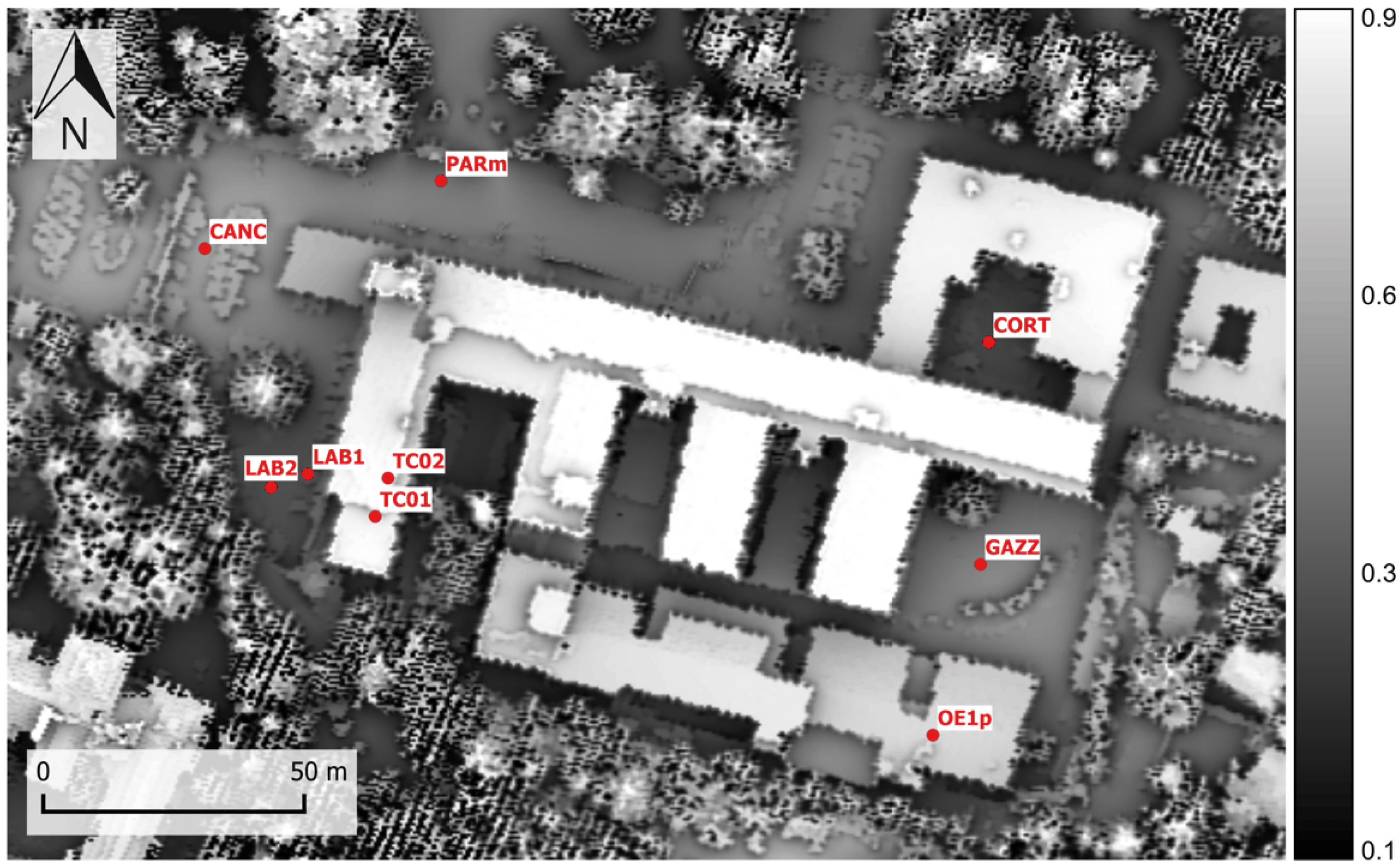
Some temperature measurements were collected simultaneously to the aerial survey at nine locations in the test area. All of the measurements are referenced to artificial surfaces, both on the ground and on building roofs.

Measurements at ground level were carried out using a thermal infrared camera FLIR P620 installed on a tripod. The short distance between the object and the sensor (about 1 m) minimized the effects of the atmosphere on the temperature measurements, making it possible to use the internal atmospheric correction model of the camera. All of the selected sites are clearly visible from the aerial images and have a homogeneous cover material. Measurements were made with constant instrument height and considering an area representative of the pavement texture. In addition, in order to control the results, a DeltaOhm datalogger equipped with a contact probe for temperature measurements was used. Furthermore, surface emissivity was assessed, following an empirical procedure (recommended by the manufacturer of the camera) that makes use of a tape with known emissivity placed on the surface and in thermal equilibrium with it. Clearly, this is a unique value of broadband emissivity over the wavelength interval where the thermal camera operates.

Temperature measurements on building roofs, instead, were collected using fixed thermocouples installed directly on roof covers; this way, it was possible to overcome logistic problems related to the access to the roofs during the limited time span available (about two hours for the entire thermal survey). The probes were installed directly on the surfaces using a thermal grease (with high thermal conductivity to maximize the heat exchange) and a high resistance adhesive tape (to avoid detachment in adverse meteorological conditions). The sampling rate of the thermocouples was set to five minutes. The collected measurements at the time of flight overpass are reported in

Table 1. Ground measurements collected in the study area. Temperatures were assessed contemporarily with the aerial flight.

Site Name	Temperature	Emissivity	Description
CANC	5.9	0.92	Clay brick pavement
CORT	7.5	0.94	Cobblestone pavement
GAZZ	7.8	0.93	Concrete block pavement
LAB1	6.6	0.95	Sett pavement
LAB2	6.1	0.96	Asphalt pavement (worn)
PARm	6.2	0.94	Asphalt pavement (fresh)
TC01	6.7	0.95	Sheath slated, flat roof
TC02	−1.6	0.95	Sheath slated, tilted roof
OE1p	3.4	0.95	Sheath slated, flat roof

.

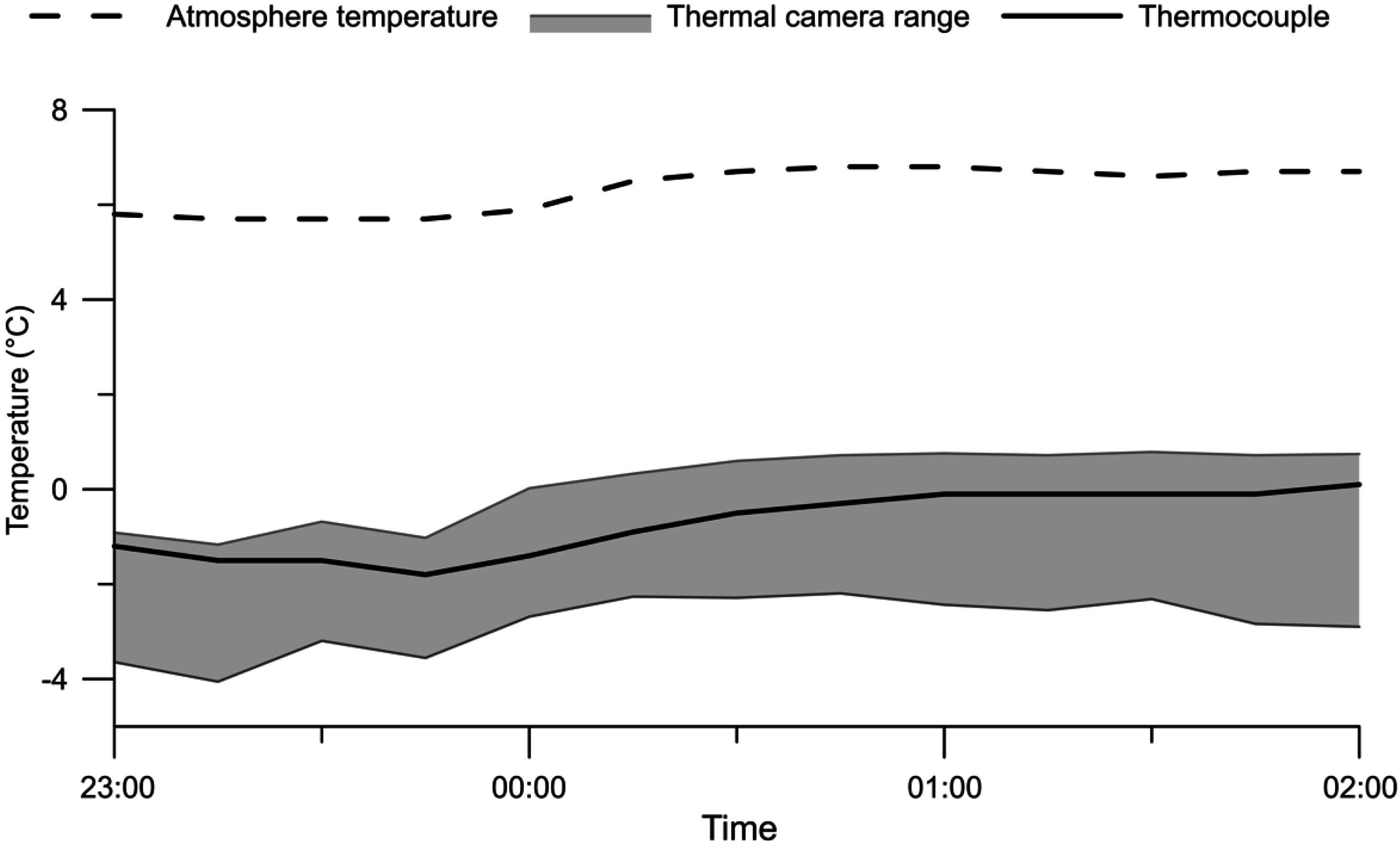
In order to evaluate the homogeneity of the surface temperature on roofs and, consequently, the representativeness of the punctual temperature measurements derived from the thermocouples, a specific survey was made during the same night of the infrared aerial acquisition. Another FLIR P620 thermal camera was installed on the roof of the School of Engineering and Architecture, in a fixed position and with a reflective covering to protect it from the solar radiation. The camera was placed on top of a high tripod (about seven meters above the roof level), and it registered images of the portion of the tilted roof covered with a sheath slated where the TC02 thermocouple was placed, with a sampling period of 15 min. These images allowed the determination of emissivity and temperature, according to the same procedure used for the other sites. The comparison between the registered temperatures is shown in Figure 2.

After the aerial flight, further surveys were made in all of the locations where temperature measurements were collected: firstly, the geographic positions were measured through GNSS techniques, computing a differential positioning with the same permanent station used for the positioning of the airplane.

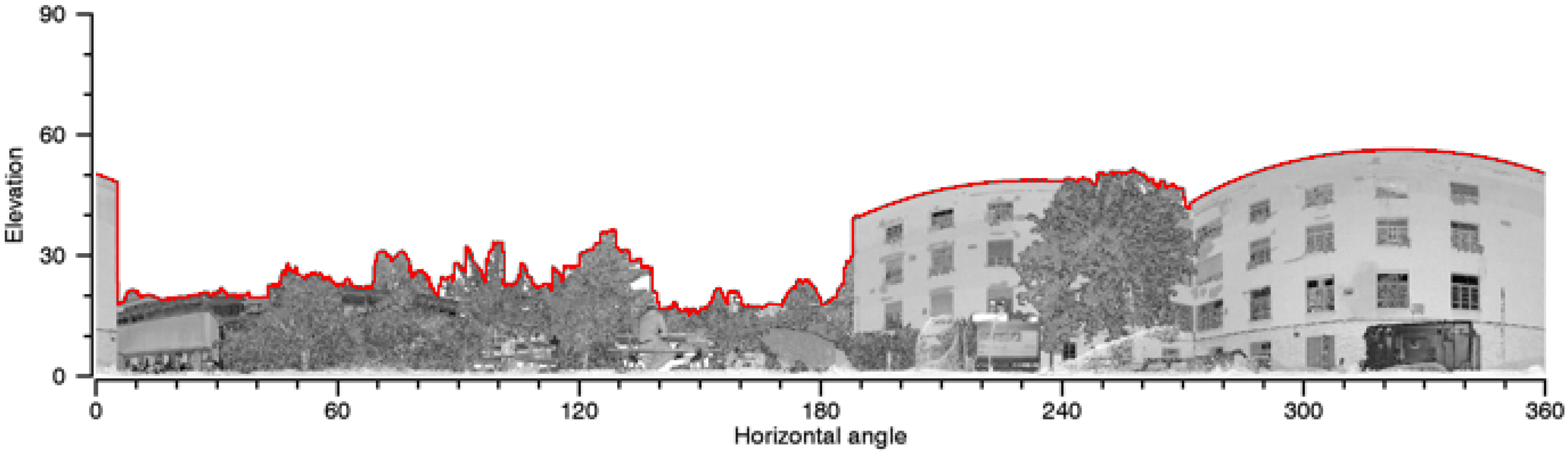
Afterwards, in the same locations, terrestrial laser surveys were performed in order to obtain 3-dimensional point clouds of all of the obstacles surrounding the measurement points and to calculate a reliable value of the sky-view factor. The instrument used is the Riegl VZ 400, a time-of-flight laser scanner characterized by an accuracy of 5 mm, a measurement range up to 600 m and a rate up to 122,000 points/s.

In each location, a scan in “panorama” pattern was performed, setting the scanner vertical thanks to the integrated inclination sensors; this surveying mode permits acquiring data covering the complete field of view of the scanner (100 degrees vertical and 360 degrees horizontal), with a scanning angular resolution of 0.04 degrees. In some scan positions, in order to cover the entire horizon line, a further scan was necessary, placing the instrument inclined using the dedicated tilt mount cradle. In this case, the alignment between the two scans was realized using reflectors placed in the area.

3.4. Ancillary Data

The emissivity map, required for the correction of the entire mosaic of aerial images, was based on the object-oriented supervised classification presented in Bitelli et al. [9], which was applied on a WorldView-2 multispectral image acquired in 2011, providing eight spectral bands at a resolution of 2 m. Five major roofing materials were distinguished: bitumen, clay, concrete, gravel and metal (

Table 2. Emissivity values assigned to the roofing materials occurring in the map derived from the classification of a very high resolution satellite image.

Roofing Material	Emissivity
Bitumen	0.95
Clay tiles	0.88
Concrete	0.90
Gravel	0.96
Metal	0.70
Other	1.00

). Where available, emissivity values were set according to field measurements, otherwise according to data published in the literature [9].

The digital technical cartography of the Municipality of Bologna at a 1:2000 nominal scale was used as the cartographic base.

The permanent GNSS station called “BOL1”, placed on the roof of the School of Engineering and Architecture, was used as the master station for all of the surveys.

4. Methods

The proposed approach for radiometric calibration of thermal imagery requires the computation of a sky-view factor map, the estimation of the atmospheric parameters and the emissivity map for the main materials occurring in the scene. The following paragraphs detail each step of the procedure.

4.1. SVF Computation

4.1.1. SVF Maps from LiDAR Data

Three open-source software products, which are able to produce continuous SVF maps starting from a DSM in grid format, were tested. Even if for biometeorological analyses the SVF is conventionally calculated at a height of one meter above the ground, for this application the SVF should be calculated at the ground level, in order to assess the amount of downwelling radiation that reaches the surface and that is then reflected in the observing direction.

The first two SVF maps were computed by the “SkyHelios” software [10]. It permits simulating the continuous sky-view factor at a fixed spatial resolution (0.5 m for the present work, as for the thermal images) for a whole area. Only a DSM of the investigated scene is required as input and, optionally, vector data about the shape and position of other obstacles lying on the ground. The calculation of the SVF is made up of three different steps: first, the scene is rendered five times with a 90° lens facing north, west, south, east and into the sky for each considered location; then, these rendered images are combined into a single sky-view image; finally, a vertex program counts the number of white pixels in this image and divides it for the total number of pixels, obtaining the value of the SVF. SkyHelios can follow two different algorithms for the computation of SVF values, namely “planar” and “spheric”, and both were tested. The difference between the two consists in the fact that in the planar method, the sphere is projected to a horizontal surface according to the cosine law.

The third SVF map was derived from the “SVF” tool developed for the ENVI-IDL™ environment [27], in the following indicated as “ENVI SVF Tool” (Figure 3). Like SkyHelios, it generates maps of the georeferenced sky-view factor with the same spatial resolution as the DSM provided as an input. The main parameters that influence the results and the running time are the spatial resolution of the DSM, the maximum search radius and the number of horizon search directions. The developers demonstrated that the number of search directions has no systematic influence on the SVF values and there are no significant differences when using more than 32 search directions (except for the edges of convex objects). However, for the present work, a number of search directions equal to 360 was used, without relevant effects on the computational time. Concerning the search radius, the developers suggested [27] using a radius of approximately the same dimension of the features to be identified on the output images. In this case, the radius was enlarged up to the maximum distance (200 m) registered by the terrestrial laser scanner during the ground surveys, in order to consider also far obstacles and therefore avoid an overestimation of the SVF value.

Finally, the software “SOLWEIG” [31] was used for the computation of the fourth SVF raster map. The software was developed as a tool for modeling the spatial variations of radiant fluxes and mean radiant temperature in complex urban settings, and in fact, the computation of the SVF is only an intermediate product. The method for the calculation is an evolution of the shadow casting algorithm [32] where, instead of using a high number of light sources with a random distribution of solar altitude and azimuth, the Sun positions are predefined and uniformly spread over the whole hemisphere (with a minor weighting for solar altitudes between 25 and 65 degrees, where the variation of hemispheric blocking from buildings usually occurs in the urban environment). In this manner, a considerably smaller number of shadow images is calculated, leading to a reduction in computational time.

All three tools were tested also considering two theoretical cases, the circular basin and the infinite canyon; the former is a circular basin surrounded by walls of the same height, while the latter is an infinitely-long canyon flanked by parallel buildings with constant height. For these two geometric arrangements, which idealize situations commonly occurring in urban environments (such as squares and long roads), the analytical solutions were published [25], and they can be used to test or compare different SVF computation algorithms [12]. In order to simulate these situations, two synthetic DSMs were generated using image processing techniques: they represent the ideal cases with a unitary height/width ratio. Both synthetic DSMs were supplied to the software applications, and after the calculation, the values obtained at the center of both the basin and the canyon were compared (

Table 3. Comparison of the sky-view factors obtained for the two theoretical cases of the circular basin and the infinite canyon, for which the analytical solutions exist.

	Infinite Canyon	Circular Basin
Analytical solution (Zakšek et al. [27])	-	0.106
Analytical solution (Oke [25])	0.447	0.200
SkyHelios-spheric	0.310	0.109
SkyHelios-planar	0.467	0.205
ENVI SVF Tool	0.305	0.108
Solweig	0.450	0.210
IDL procedure ($F_{\mathsf{\Omega }}$)	0.295	0.106
IDL procedure ($F_L$)	0.447	0.200

).

4.1.2. SVF from the Terrestrial Laser Scanner

In order to check the accuracy of the raster maps produced by LiDAR data, the SVF was derived also exploiting the dense point clouds acquired by the terrestrial laser scanner. In this case, punctual values instead of maps could be computed, at those locations where the surface temperature was measured.

An automatic routine was developed in IDL™ to process the point clouds. Firstly, point coordinates, which were expressed in a local Cartesian system centered on the instruments, were translated upward to accommodate for the height of the origin of the scanner system from the ground; this translation is the sum of the vertical offset of the instrumental center from its base (determined in the laboratory by means of topographical measurements) and, when used, the height of the tripod. Then, the coordinates were expressed in a spherical system centered on the observation point. Both azimuthal and polar directions were divided in steps by 0.1 degrees. For each angular step, the echo from the closest object was identified, and its range and amplitude were stored in an array. This way, it is possible to reconstruct a 2D view (azimuth and elevation) of the obstacles visible all around each point and, therefore, determine their maximum elevation as a function of the azimuthal direction. This function ($\mathsf{\beta }=\mathsf{\beta }\left(\mathsf{\varphi }\right)$) was used to solve Equations (7). Isolated pixels in the 2D view were removed as they may originate from incidental echoes caused by flying birds or instrumental noises. An example is shown in Figure 4.

A comparison of the values obtained with the different techniques and software solutions is reported on

Table 4. Sky-view factor values obtained from LiDAR and terrestrial laser scanner data for the calibration and control sites.

Site	DSM LiDAR				Terrestrial Survey
	Sferic	Planar	ENVI	Solweig	${\mathit{F}}_{\mathit{L}}$	${\mathit{F}}_{\Omega }$
CANC	0.55	0.79	0.55	0.79	0.52	0.76
CORT	0.24	0.41	0.24	0.41	0.22	0.38
GAZZ	0.51	0.72	0.51	0.72	0.49	0.70
LAB1	0.25	0.40	0.24	0.38	-	-
LAB2	0.28	0.46	0.28	0.46	0.23	0.40
PARm	0.40	0.59	0.40	0.58	0.43	0.63
TC01	0.74	0.89	0.74	0.89	0.75	0.92
TC02	0.87	0.97	0.87	0.97	0.85	0.96
OE1p	0.75	0.92	0.74	0.92	0.71	0.89

.

Furthermore, this procedure was tested for the two ideal cases of the circular basin and the infinite canyon (Table 3). In these cases, two simulated point clouds were generated, with the same angular step of the “panorama” scanning mode adopted for the surveys, assuming a unitary height/width ratio for the geometry of obstacles.

4.2. Atmospheric Parameters Determination

The atmospheric parameters necessary for the derivation of the surface temperature were estimated through a least square adjustment procedure, using the measurements of temperature, emissivity and sky-view factor acquired at the five points considered as calibration sites (labeled CANC, CORT, LAB2, TC01 and OE1p in Table 1).

For each point, one equation of the type of Equation (1) (with $l_{sr}=l_b$) can be written. Given the assumption of negligible lateral variation of the atmospheric conditions, a system with only three unknown parameters ($\mathsf{\tau }$, $L_u$, $L_d$) can be obtained; thus, three is the minimum number of ground observations necessary to retrieve the solution. In this case, the use of five points with varying emissivity values (different materials) and SVFs (points located on the ground and roof levels) allows a slight redundancy and permits a basic control over the solution quality. Clearly, when analyzing wider and more complex areas, a higher number of measurements (possibly with varying parameters) is recommended in order to preserve the accuracy, always reaching a compromise between redundancy and the logistics of the surveys, which must be performed synchronously with the flight.

Since the product of transmittance and downwelling radiance appears, the equations were linearized through a Taylor expansion truncated at the first order. Each line of the system can be written as follows,

$$\left[\mathsf{ϵ}{l}_B+\mathsf{\rho }F{L}_d^0+\mathsf{\rho }\left(1-F\right)l_B\right]d\mathsf{\tau }+d{l}_u+\left({\mathsf{\tau }}^0\mathsf{\rho }F\right)d{l}_d=l_S-l_S^0$$

(8)

where the apex ${}^0$ designates approximated values of the parameters and $d\mathsf{\tau }$, $d{l}_u$ and $d{l}_d$ are the unknown corrections to be summed to the approximated values. The procedure is iterative and generally converges in very few runs.

The solution was computed with a bounded least square procedure, in order to force the retrieved parameters to be positive (the code uses the Bounded-Variables Least-Squares (BVLS) routine by Michele Cappellari, available at http://purl.org/cappellari/software). The spectral band in which the thermal camera is sensitive was discretized in steps of 0.1 microns, and the system was solved for each wavelength step. The whole procedure was implemented in IDL™.

The estimation was repeated to test both the sky-view factor sets derived by Equation (7).

4.3. Surface Temperature Retrieval

The model presented in Equation (3) was implemented in the ENVI-IDL™ environment. The procedure generates the image of the surface temperature, starting from the image of apparent (at sensor) temperature acquired by the aerial platform, working on raster datasets on a pixel per pixel basis. The required inputs are the image of the apparent temperature, the atmospheric parameters estimated by the least square adjustment, a raster map of the surface emissivity and an SVF map. The left side term of Equation (3) is computed; then, the surface temperature is derived from a look-up table, which can be built by fitting a second order polynomial relation between the radiance integral and temperature [9].

The surface temperature retrieval was repeated using all of the sets of SVF values computed by the different methods presented in Section 4.1. The differences were analyzed, and a first assessment of the accuracy was performed using a set of four control points (labeled GAZZ, PARm, TC02 and LAB1 in Table 1), where temperature was measured on the ground.

5. Results

Using the measurements performed at five calibration points, two sets of atmospheric parameters (transmittance, upwelling and downwelling radiances) were estimated. The two sets differ only for the definition of the sky-view factor, according to Equations (7). The values obtained with the two definitions do not vary significantly (less than 2%) and, in both cases, the RMS of the difference between the surface temperature computed with the retrieved parameters and the one measured on the ground at the calibration points does not exceed 1.3 °C (

Table 5. Surface temperature values of the calibration points, resulting from the least square adjustment for the computation of atmospheric parameters. Differences and RMSs are referenced to the temperatures measured on the ground.

Site	Measured	Computed			Difference
		$\mathit{F}=1$	${\mathit{F}}_{\mathit{L}}$	${\mathit{F}}_{\Omega }$	$\mathit{F}=1$	${\mathit{F}}_{\mathit{L}}$	${\mathit{F}}_{\Omega }$
CANC	5.9	6.1	7.1	6.6	0.2	1.2	0.7
CORT	7.5	9.2	8.2	8.2	1.7	0.7	0.7
LAB2	6.1	8.0	6.9	7.1	1.9	0.8	1.0
TC01	6.7	3.7	4.3	4.4	−3.0	−2.4	−2.3
OE1p	3.4	2.4	2.9	3.0	−1.0	−0.5	−0.4
RMS:					1.9	1.3	1.2

). The RMS rises significantly (1.9 °C) if an SVF equal to one is assumed for all points, which means neglecting the SVF and the effects of the geometry of the observed surfaces.

Using the digital surface model, four SVF maps were produced over the test area. The solutions generated by Solweig and SkyHelios-planar show a coherent statistical behavior: a median value of 0.52 and 0.55, respectively, with an Interquartile Range (IQR) of 0.45 and 0.47. Analogously, the ENVI SVF Tool solution is in good agreement with the SkyHelios-spheric one, with median values of 0.36 and 0.38, respectively (IQR of 0.39 and 0.41). Both SkyHelios-planar and spheric algorithms provide higher values of SVF if compared to their counterparts.

Surface temperature maps of the test area were produced using all four SVF solutions described in Section 4.1.1. A first check over the accuracy of the temperature retrieval process was performed considering four control points (three at the ground level and one at the roof level), where the temperature was directly measured at the same time as the flight. The results are reported in

Table 6. Surface temperatures derived by the radiometric processing of thermal images using different maps of SVF and differences with the measured values at the control sites.

Site	Measured	Computed					Difference
		None	Spheric	Planar	ENVI	Solweig	None	Spheric	Planar	ENVI	Solweig
GAZZ	7.8	9.1	7.1	7.9	7.1	7.9	1.3	−0.7	0.1	−0.7	0.1
PARm	6.2	8.2	6.1	6.8	6.1	6.8	2.0	−0.1	0.6	−0.1	0.6
TC02	−1.6	0.1	−0.3	0.0	−0.3	0.0	1.7	1.3	1.6	1.3	1.6
LAB1	6.6	9.3	7.1	7.5	7.1	7.5	2.7	0.5	0.9	0.5	0.9
RMS:							2.0	0.8	1.0	0.8	0.9

, showing also a solution that does not consider the SVF (labeled as “none” in the table).

6. Discussion

Ground measurements of temperature and emissivity play a major role in the approach proposed. Since these measurements involve the use of both thermal cameras and thermocouples fixed on the investigated surfaces and considering that these instruments are based on completely different technologies, the agreement between these two kinds of data was verified during the continuous monitoring described in Section 3.3 at the site labeled “TC02”. As shown in Figure 2, thermocouple records always fall within the temperature range recorded by the thermal camera, once the emissivity of the material is properly set; the difference in temperature between thermocouple readings and thermal image averages does not exceed 1°C and is generally lower than 0.5.

The atmospheric parameters were computed through a least square adjustment. It is important to point out that, even if these parameters have a clear physical meaning according to Equation (1), they may be highly affected by systematic errors if present in the measurements. Furthermore, although they are computed as spectral quantities depending on the wavelength, they cannot reflect the real dynamics of gaseous absorption and emission at each wavelength; thus, their values can assume a physical meaning only when integrated over the entire interval in which the thermal sensor operates. In any case, the parameters are strongly dependent on the radiometric quality of aerial thermal images and on the accuracy of the ground surveys: this is the major limitation of the proposed approach. However, this may be regarded also as a strength if the overall accuracy of surface temperature retrieval is considered.

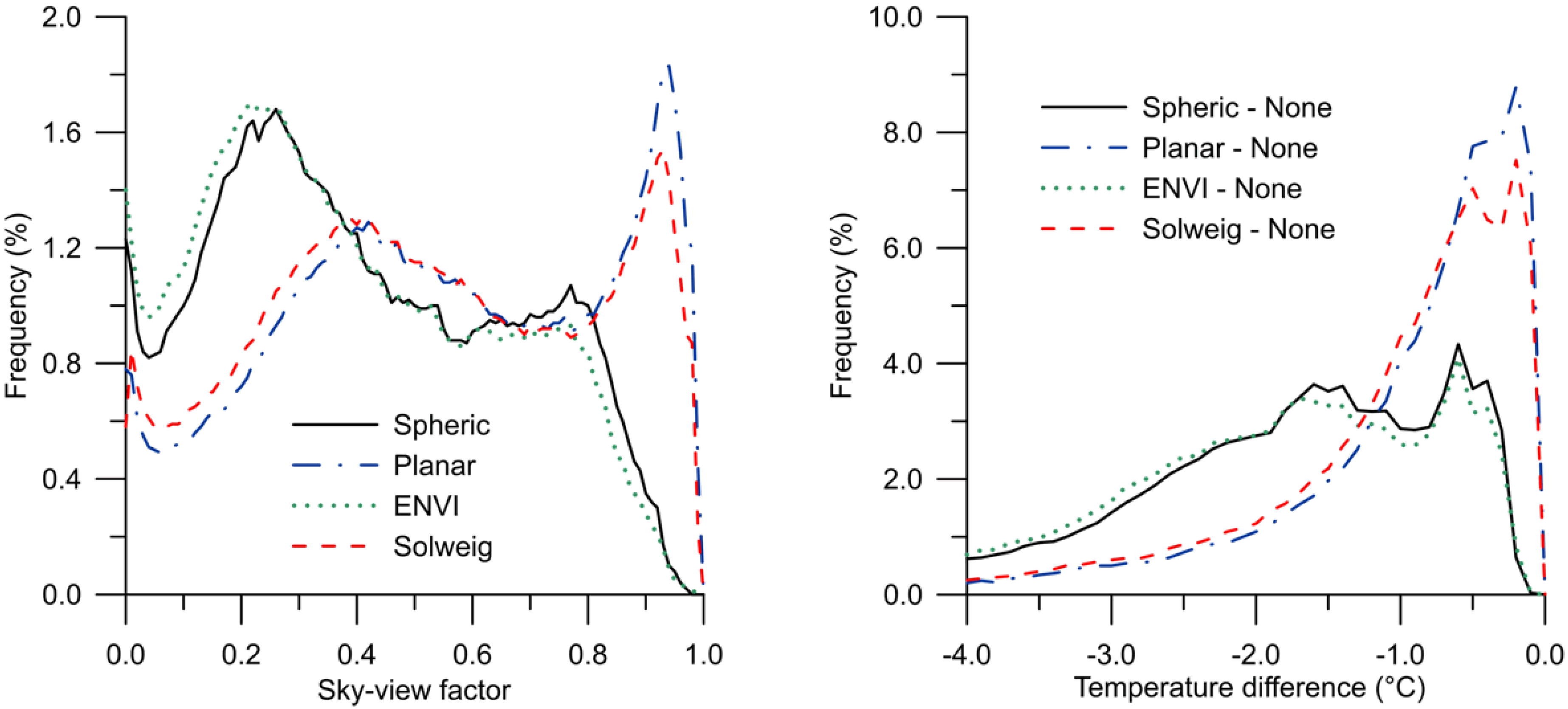
Looking at the histograms reported in Figure 5 (left), it is evident that the four examined methods for the SVF computation provide significantly different results, even if the trends look similar all over the test area and, in particular, over artificial surfaces. Notably, every approach is characterized by a bi-modal distribution, probably corresponding to roofs and street surfaces, but there are systematic biases among them. The map obtained from the SkyHelios-planar algorithm generally shows the highest SVF values.

These statements are confirmed also by the results for the theoretical cases, shown in Table 3: the values obtained at the centers of the circular basin and the infinite canyon are almost equal between the SkyHelios-planar algorithm and the Solweig one and between the SkyHelios-spheric method and the ENVI SVF Tool; differences with analytical solutions are lower than 2% in both cases, in good agreement with the outcomes of previous studies [13]. In practice, the algorithms seem to reproduce the ambiguity between the different definitions of the SVF: in fact, some evident similarities can be found between histograms of the “planar” SVF computed from SkyHelios and the one from Solweig (Figure 5 (left)); in a similar way, the results of the ENVI SVF Tool reproduce the trend of the “spheric” SkyHelios SVF. Furthermore, the IDL™ code, used for the processing of terrestrial laser data, produces values in very good agreement with both the analytically-derived values and the ones extracted from the SVF maps on the same points (Table 4).

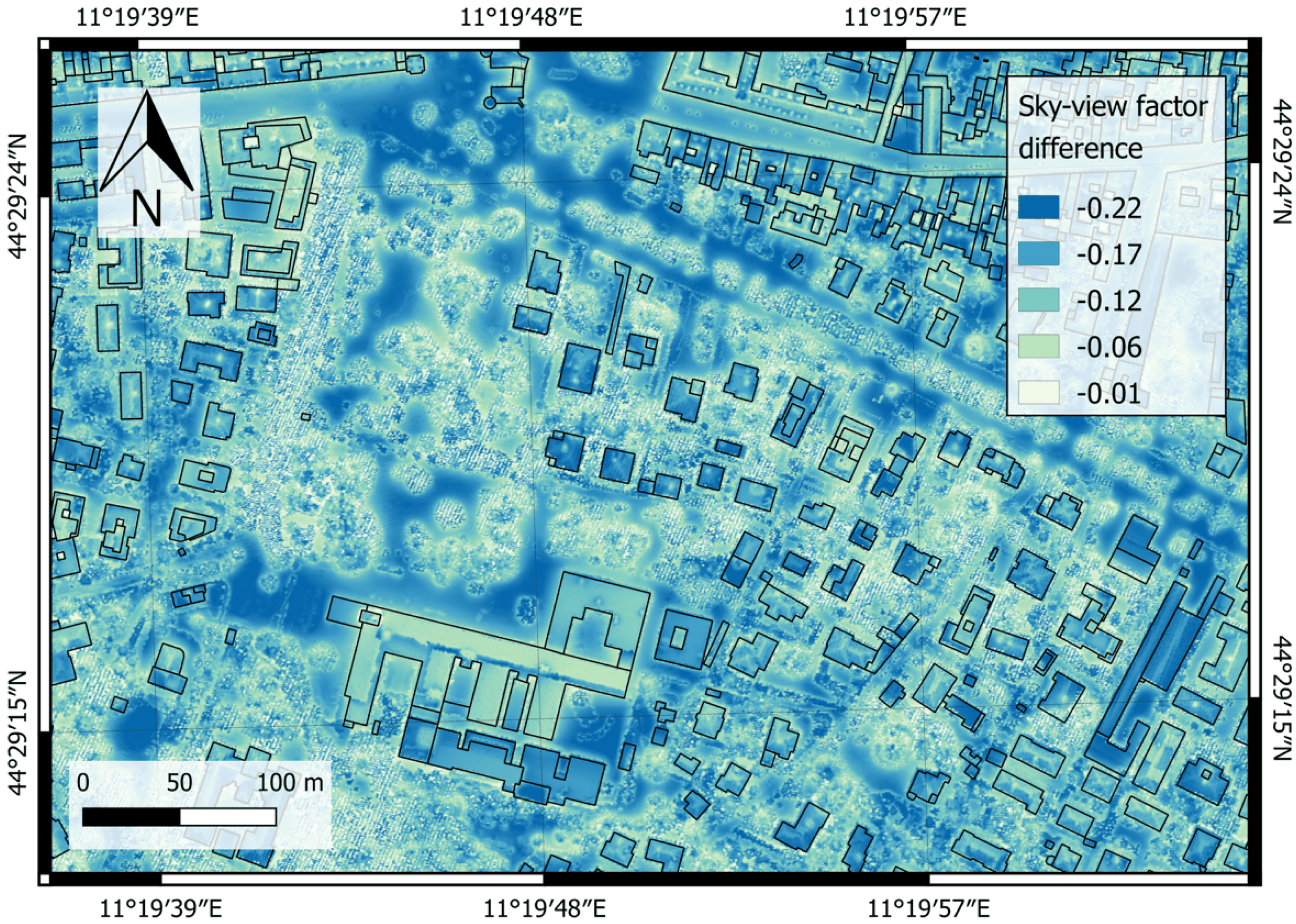
Looking at the temperature residuals of the four check points reported in Table 6, it can be observed that without considering the SVF, the RMS error of the solution is comparable to the one obtained in previous studies (2.6 °C in Ren et al. [33] and 2.1 °C according to the best solution in Bitelli et al. [9]). Taking into account the SVF, instead, appears to improve significantly the accuracy of the retrieved temperatures, proving the valuable contribution that a high quality DSM, such as the one that can be obtained from a LiDAR survey, can offer to the whole process. Among the four SVF maps exploited, no significant differences on corrected temperatures were found, even if a slightly lower RMS (about 0.8) was obtained with SkyHelios-spheric and ENVI SVF Tool solutions if compared to SkyHelios-planar and Solweig ones (about 1.0 °C). These differences in temperature are minimal, even if the differences in SVF values are pronounced (Figure 6).

The effects of using the different SVF maps for the surface temperature retrieval process can be observed also in Figure 5 (right). As can be seen, SVF values lower than one always produce a decrease in temperature. The amount depends on the method adopted, ranging from about 0.7 °C in the median, using SkyHelios-planar SVF, to about 1.8 °C, using the ENVI SVF Tool. Neglecting a few spurious pixels in which the differences are higher than 10 °C, also the IQR is larger with the ENVI SVF Tool (1.8), and it is minimal in the case of the planar method (1.0).

On the whole, the results of the proposed approach, which is based on an adjustment, suggest that the absolute values of the SVF are not so relevant; what is important is that this parameter relatively quantifies to what extent each surface is exposed to the open sky, distinguishing, for example, the obstructed view of road pavement in a street canyon from the open view of the roof of a high building. This is not true when the procedure involves a rigorous modeling of the radiative transfer in the atmosphere.

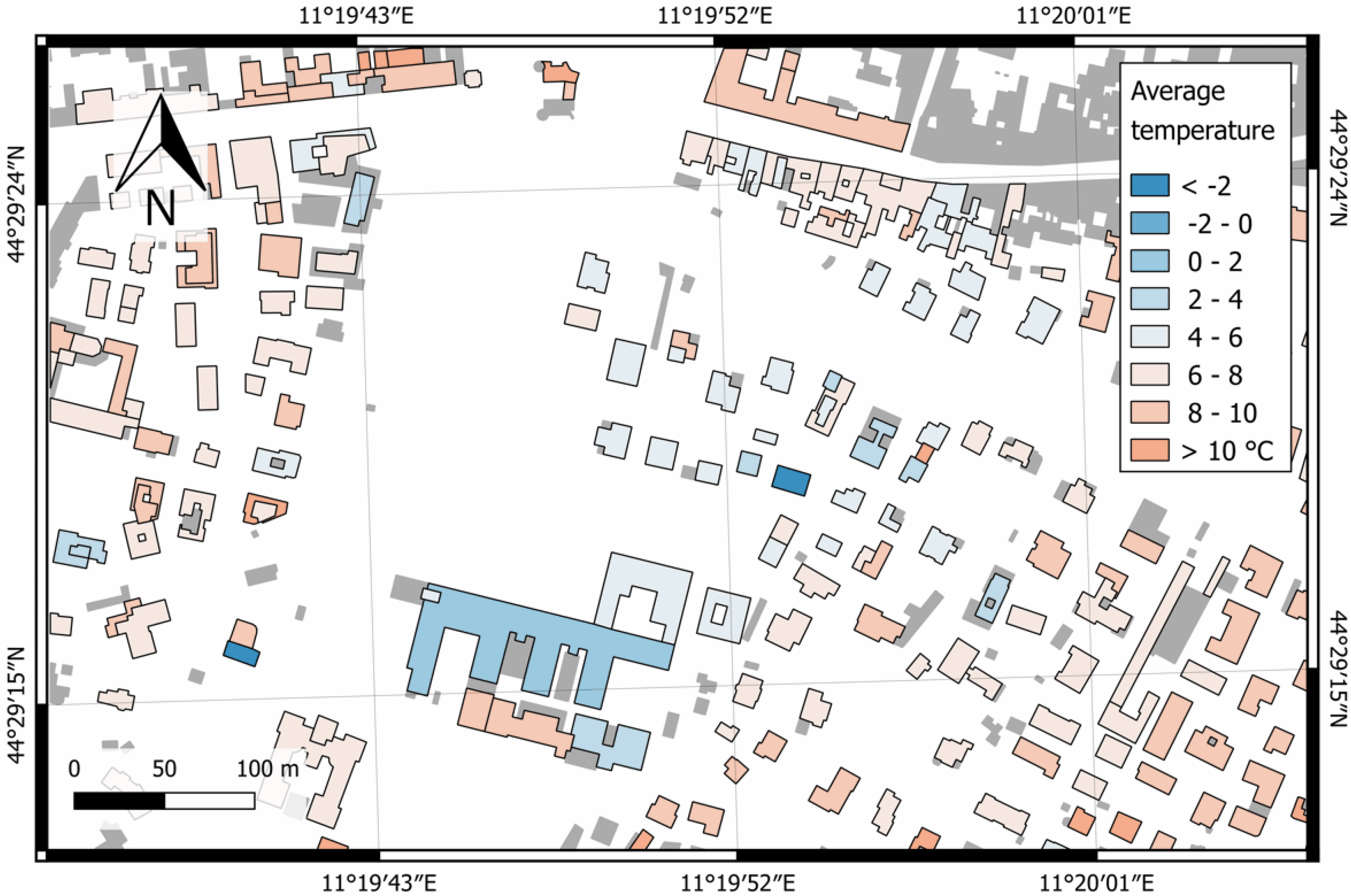
An example of the possible outputs of the proposed procedure is shown in Figure 7. The surface temperature map obtained from aerial images was imported in a GIS environment and coupled with the numerical cartography. The average temperature of roofs was therefore calculated and assigned as an attribute to the building entities.

This study focused mainly on the integration of different data sources for the computation of atmospheric parameters and SVF, but it is worth mentioning that the surface temperature retrieval process is highly affected by emissivity. As demonstrated by previous studies, a variation of 1% in emissivity can produce a variation in temperature of about 0.3 °C [9], which is generally higher than the one related to the SVF itself. Furthermore, if the effects of multiple reflections among the complex surfaces of an urban environment are considered, the effective emissivity may differ from the emissivity of the material, and a correlation between SVF and effective emissivity can be found [34]. Thus, emissivity is likely to be the major source of uncertainty in surface temperature mapping, especially considering the large variability of materials occurring in an urban environment and the variability of emissivity values even for the same material, due to aging and weathering [23,35]. For the present work, emissivity values are directly measured for the calibration and control points, and they can be considered valid for those locations. However, a higher number of samples would be required to fully represent the variability that can occur within the urban texture.

Finally, it is important to note that all of the approaches adopted for the SVF calculation rely on the assumption of isotropic downwelling radiation, which is not realistic in general [36]. A possible future development might be the modeling of the directional behavior of radiance coming from the sky and the surrounding objects, also by integrating data from thermal sensors installed on Unmanned Aerial Vehicles (UAVs), capable of acquiring tilted views of vertical surfaces. The use of recently-developed sensors installed on UAVs might prove of great interest for energetic applications in urban areas. In fact, they usually have a wider field of view, thus permitting flight at lower heights and limit atmospheric effects on the acquired imagery, even if the geometric distortion could be greater. On the other hand, the surveying of wide areas in a limited time span would require the simultaneous use of a fleet of UAVs.

7. Conclusions

A single-channel surface temperature retrieval method was proposed, which exploits the integration of aerial thermal images with LiDAR data and ground surveys, in order to achieve a better accuracy. The model required an SVF map, which was derived from LiDAR data, using four software solutions published in the literature. The obtained values compare well (differences lower than 3%) with the ones derived from several terrestrial laser scanner surveys performed on the ground or on top of buildings. A specific procedure was developed in the present work to calculate the SVF from the point cloud acquired from a scan position, according to different theoretical definitions.

At the same locations, measurements of surface temperature and emissivity were performed (at the same time of the aerial thermal survey), involving the combined use of thermal cameras and thermocouples. The agreement between the two instruments, based on completely different technologies, was verified by a continuous monitoring of a roof surface performed on the same night of the flight. These ground surveys were used to estimate the atmospheric parameters involved in the model (through a bounded least square adjustment) and for a first assessment of the accuracy of the results.

The RMS of the difference between the surface temperatures computed from the model and measured on the check sites ranges between 0.8 and 1.0 °C, depending on the algorithm used to calculate the sky-view factor. Results are in general better than the ones obtained without considering SVF and prove the effectiveness of the integration of different data sources. The uncertainty related to the SVF determination appears to be of a lower magnitude than the one due to the emissivity, because of the great variety of materials occurring in an urban environment and the variability of emissivity even for the same material, as a consequence of aging and weathering effects.

On the one hand, the use of some ground measurements in the approach proposed has the advantage of avoiding the rigorous radiative transfer modeling through the atmosphere, which is often difficult to achieve with the desired accuracy, since detailed data on the whole atmosphere column above the investigated area are rarely available. On the other hand, this approach is highly dependent on the accuracy and representativeness of the data measured on the ground.