Retrieval of Seasonal Leaf Area Index from Simulated EnMAP Data through Optimized LUT-Based Inversion of the PROSAIL Model

Abstract

The upcoming satellite mission EnMAP offers the opportunity to retrieve information on the seasonal development of vegetation parameters on a regional scale based on hyperspectral data. This study aims to investigate whether an analysis method for the retrieval of leaf area index (LAI), developed and validated on the 4 m resolution scale of six airborne datasets covering the 2012 growing period, is transferable to the spaceborne 30 m resolution scale of the future EnMAP mission. The widely used PROSAIL model is applied to generate look-up-table (LUT) libraries, by which the model is inverted to derive LAI information. With the goal of defining the impact of different selection criteria in the inversion process, different techniques for the LUT based inversion are tested, such as several cost functions, type and amount of artificial noise, number of considered solutions and type of averaging method. The optimal inversion procedure (Laplace, median, 4% inverse multiplicative noise, 350 out of 100,000 averages) is identified by validating the results against corresponding in-situ measurements (n = 330) of LAI. Finally, the best performing LUT inversion (R² = 0.65, RMSE = 0.64) is adapted to simulated EnMAP data, generated from the airborne acquisitions. The comparison of the retrieval results to upscaled maps of LAI, previously validated on the 4 m scale, shows that the optimized retrieval method can successfully be transferred to spaceborne EnMAP data.

1. Introduction

In order to ensure the supply of the future world population with agricultural goods (food, fiber and energy), a sustainable increase in agricultural productivity and an associated reduction of the yield gap [1] is mandatory. This requires the introduction of optimized agricultural management strategies [2]. Since landscape-scale vegetation mapping requires expensive and time-consuming field surveys, remote sensing offers an alternative which is both time- and cost-effective [3]. The German satellite mission EnMAP (Environmental Mapping and Analysis Program), to be launched in 2018, will provide high-quality calibrated hyperspectral data allowing an improvement of already existing methods and the development of new strategies for the retrieval of geochemical, biochemical and biophysical parameters. Further, the retrieved information will support analyses of ecological processes and the generation of multitemporal spatial information products [4].

The scientific aim of the presented study was to investigate the impact of different selection criteria in the model inversion process of the PROSAIL model and to assess whether it is possible to gain information about seasonal development of biophysical land surface parameters on the regional scale using spaceborne imaging spectroscopy without being dependent on in-situ data. The investigation of the seasonal development of LAI was the subject of recent studies (e.g., [5]). Due to the lack of hyperspectral satellite data, most of them were based on multispectral and medium resolution imagery (e.g., [6,7]). In this study, we examine whether the retrieval of biophysical parameters is possible using a unified but still robust method, which is successfully applicable for different crops at different times with different illumination geometry, and must not be adapted to individual acquisitions. Preparing for the use of spaceborne hyperspectral data, which potentially is collected globally, an overall scientific objective should be to derive this information without depending on prior information in the form of in-situ data. This is mostly due to the fact that an implementation of corresponding field measurements, as it has regularly been observed with spatially and temporally limited airborne spectroscopy campaigns (e.g., [8,9,10]), would not be viable in the context of the satellite-based EnMAP. This study focuses leaf area index (LAI) as it is a significant parameter describing the size of the producing layer and it is also important for the estimation of foliage cover, as well as for forecasting crop growth and yield [11,12]. Investigation of LAI thus potentially promotes the understanding of biophysical processes in canopies.

The widely used PROSAIL model, which is coupled from the leaf optical properties model (PROSPECT) and the canopy bidirectional reflectance model (SAIL) [13], was applied to simulate reflectance for homogeneous vegetated surfaces [14]. In contrast to empirical statistic models, such as vegetation index correlations, which have to be calibrated against in-situ data if they are to be used for the quantitative derivation of biophysical parameters (variable-driven), physically based methods can potentially be applied to quantitatively derive biophysical parameters without the availability of in-situ data (radiometry-driven). Due to their intrinsic dependency on in-situ data, well-trained empirical models may deliver high-quality results, but at the same time suffer from very limited transferability. In addition, vegetation indices are limited due to the fact that they are not originally a measure for one isolated specific variable, such as chlorophyll content, since the reflected signal is influenced by the interaction of several biophysical and biochemical components. The inversion of a reflectance-generating physically based model, by contrast, enables the determination of several biophysical parameters at the same time [15] by taking the continuous reflectance signal into account, e.g., by the use of a look-up table (LUT). Other approaches use radiative transfer models to train inverse models (e.g., support vector machines, artificial neural networks). Depending on their nature, empirical retrieval methods are classified as variable-driven, while physically-based approaches are classified as radiometry-driven according to Baret & Buis [16].

Due to their calibrated nature, empirical methods are sensitive to anisotropy effects that result from a variable sun-sensor-target geometry within and between remote sensing data sets. Accounting for anisotropies such as the bidirectional reflectance distribution function (BRDF) of different surface types is of utmost importance in regard to the expected ±30° pointing capability of EnMAP. Exploiting the capabilities of the future EnMAP mission thus requires the application of physically based approaches that may explicitly account for these anisotropies. Illumination angle dependent nonlinearities thus may serve as additional information, e.g., for constraining model parameters, instead of being an error source. An interpretation of the BRDF can be integrated into the retrieval strategy, thereby improving the overall retrieval quality. Such models have previously been applied to agricultural crops and grasslands in the scope of airborne campaigns (e.g., [17,18]). The aim of this study consequently is to determine the impact of different selection criteria in the model inversion process and to apply the optimized method for the retrieval of seasonal LAI without prior information. The very general nature of the approach, which does not include band selection or parameter constraints, allows the transfer of the found optimized approach to data that corresponds to the expected spatial, temporal and spectral characteristics of the future EnMAP mission.

2. Material & Methods

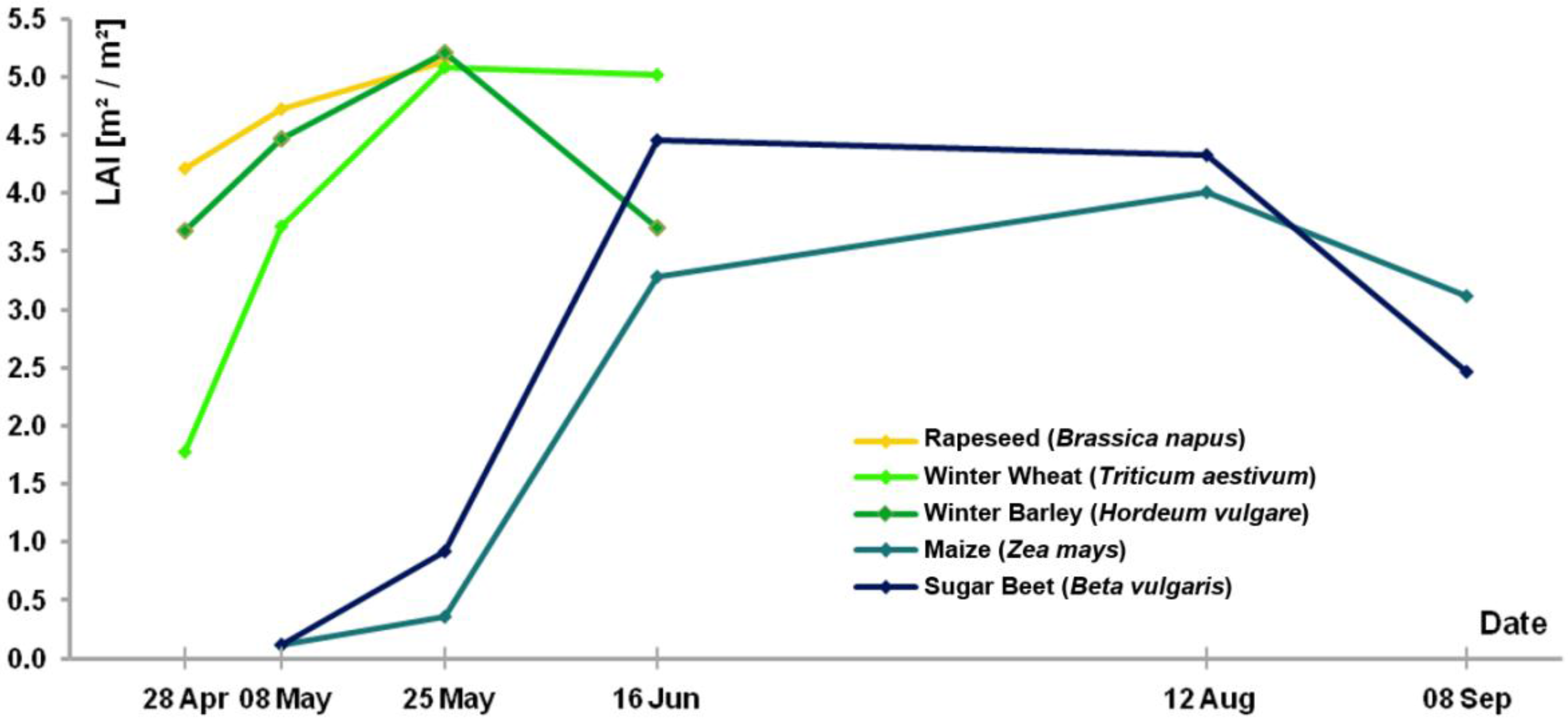
2.1. Introduction to the Study Area

To compensate for the non-availability of EnMAP data until 2018, when the system is expected to be launched, an alternative database was compiled for the implementation and examination of retrieval strategies. The airborne imaging spectrometer AVIS-3 (Airborne Visible and Near Infrared Spectrometer, LMU, Munich, Germany), developed at the Department of Geography of the Ludwig Maximilian University (LMU) [19], was used to perform four imaging flights during the course of the vegetation period of 2012 over a 12 km² large test site in Southern Germany (Neusling, Lower Bavaria, central coordinates: 48.69°N, 12.87°E). The seasonal campaign was complemented by two additional acquisitions from the airborne sensor HySpex, which is operated by the German Aerospace Center (DLR) [20].

Figure 1 presents the locations of elementary sampling units (ESU), which were defined for the flight-parallel ground measurements. In order to gain a representative sample, emphasis was placed on a meaningful distribution of the ground sampling points, which should ideally allow the detection of potential heterogeneities within individual fields on the one hand, while trying to capture as many fields as possible on the other. Moreover, a distance of at least 20 m between each ESU was assigned in order to prevent the recording of redundant information when allocating the in-situ to the airborne data. Further, Table 1 gives an overview of all six airborne data acquisitions in 2012.

Figure 1. Locations of the elementary sampling units, presented as collected LAI values, for the six airborne acquisition dates (UL: 28 April 2012, UR: 8 May 2012, ML: 25 May 2012, MR: 16 June 2012, LL: 12 August 2012, LR: 8 September 2012). Fields that are cultivated with the crops investigated in this study (rapeseed, winter wheat, winter barley, sugar beet, maize) are highlighted in greenish colors. Field boundaries are displayed in yellow.

Figure 1. Locations of the elementary sampling units, presented as collected LAI values, for the six airborne acquisition dates (UL: 28 April 2012, UR: 8 May 2012, ML: 25 May 2012, MR: 16 June 2012, LL: 12 August 2012, LR: 8 September 2012). Fields that are cultivated with the crops investigated in this study (rapeseed, winter wheat, winter barley, sugar beet, maize) are highlighted in greenish colors. Field boundaries are displayed in yellow.

Table 1. Airborne data acquisitions over the Neusling test site.

Acquisition Date	Sensor	Sun Zenith (°)	Sun Azimuth (°)
28 April	AVIS-3	42	132
8 May	HySpex	45	115
25 May	AVIS-3	39	236
16 June	AVIS-3	28	146
12 August	HySpex	42	133
8 September	AVIS-3	45	155

Table 1. Airborne data acquisitions over the Neusling test site.

Acquisition Date	Sensor	Sun Zenith (°)	Sun Azimuth (°)
28 April	AVIS-3	42	132
8 May	HySpex	45	115
25 May	AVIS-3	39	236
16 June	AVIS-3	28	146
12 August	HySpex	42	133
8 September	AVIS-3	45	155

In order to validate the methods developed for the retrieval of biophysical parameters, an extensive field campaign was carried out alongside the airborne data acquisitions, resulting in more than 330 valid LAI measurements of five different crops. These represent the major crops cultivated in the area (winter wheat, winter barley, rapeseed, maize, sugar beet). The LAI measurements were conducted non-destructively using LAI-2000 plant canopy analyzers (Li-Cor, Lincoln, NE, USA), applying a diagonal sampling pattern (two reference and eight canopy measurements) within elementary sampling units corresponding to the geometric resolution of the airborne data.

2.1.1. Data Preprocessing

The preprocessing of the airborne data, which also was carried out at LMU for the AVIS-flights, includes analysis of the spectral properties, sensor calibration, geometric correction, spatial data fusion, radiometric calibration and finally spectral data fusion. Using in-situ measurements conducted with a calibrated ASD FieldSpec 4, the raw data was finally calibrated to bottom of atmosphere (BOA) reflectance by empirical alignment. Having gone through all corrective steps, AVIS-3 data consists of 197 spectral bands, covering a spectral range from 477–1704 nm at a spectral resolution of 5.8 nm (<994 nm) and 6.6 nm (>994 nm), respectively. The ground sampling distance (GSD) in this case was 4 m. An important step of the preprocessing is the consideration of viewing angle information. For this purpose, sensor zenith and azimuth angle were stacked to the spectral data as additional bands. If this meta information is available in conjunction with the respective solar zenith angle of the acquisition time, the illumination geometry can be traced for each pixel.

The HySpex data was acquired and preprocessed by DLR, atmospherically corrected by the use of ATCOR [21], and provided as BOA reflectance with a GSD of 4 m, equal to the AVIS-3 data. The spectral properties of HySpex were adapted to those of AVIS-3, according to the spectral response functions of the latter, which is assumed to correspond to a Gaussian distribution around the center wavelength of each band. This results in a full width half maximum (FWHM) equal to the sampling interval of the sensor. Further, sensor zenith and azimuth information was added as separate bands to the HySpex data in order to conform to the specifications of the processed AVIS-3 data.

2.1.2. Data Transfer to EnMAP Scale

To examine the applicability of the methods investigated in this study to the upcoming EnMAP-Hyper Spectral Imager (HSI), the airborne hyperspectral datasets of the study site had to be modified to meet the spatial, spectral and radiometric properties of the future satellite sensor. For that purpose, Segl et al. [22] have developed the EnMAP End-to-End Simulator (EeteS), by which the image data from the multiseasonal campaign was converted into simulated EnMAP data. During forward simulation, EeteS uses several modules for the simulation of atmospheric effects and sensor properties (radiometric, spectral and spatial) and converts the airborne reflectance to realistic raw top of atmosphere (TOA) data. It is coupled with the backward simulation tool encompassing on-board L1-calibration of non-linearity and dark current correction as well as absolute radiometric calibration. The radiometric module converts the data from at-sensor radiance to digital numbers by taking into account a range of influence parameters, such as integration time, quantum efficiency (QE), different kinds of noise, infrared background signal, high/low gain modes for the VNIR detector, variable offsets and gains, as well as an individual non-linear response for each detector element. This is an important step, because these parameters define the sensor-dependent noise, as specified by the detector manufacturer. The subsequent L2-processors of co-registration, atmospheric correction and ortho-rectification complete the tool. This allows the generation of artificial satellite data, which incorporates the instrumental and environmental configurations of the future EnMAP-HSI.

It should be noted that the EnMAP simulations used in this study are restricted to spectral information within the spectral range of AVIS-3, i.e., from 471–1753 nm. Although the simulation includes the full EnMAP spectral range (420–2450 nm), all bands in the simulated data below 471 and beyond 1753 nm contain no information.

2.2. Parameter Retrieval through Look-Up Table Inversion

To estimate biophysical parameters from spectral reflectance data, all physically based radiative transfer (RTM) models have in common that they must be inverted [15]. There are several inversion techniques described in the literature, which differ in computation speed, robustness and performance. The most common inversion techniques for parameter retrieval are numerical optimization algorithms, training of artificial neural networks (ANN) with RTM data, which by far represents the computationally fastest method, and look-up tables (LUT) [23].

The quality of a LUT depends on the range, discretion levels, number of parameter configurations as well as on an optimal search strategy [24]. If the distance between the discretion levels is too far or the dimension is too low, the LUT inversion may lead to suboptimal solutions [23]. Similar to neural networks, which have to be trained before parameter retrieval, an advantage of the LUT is that a large amount of the computing time is completed before the actual application. This antecedent calculation is based on various input parameters [24]. In contrast to numerical optimization and also to ANNs, the LUT approach admits a global search and is in this way not in danger of being trapped in local minima [25].

Numerous studies, e.g., [26,27], showed that the LUTs are often more robust and generate higher accuracies compared to other RTM inversion approaches. Moreover, LUTs have the advantage that they represent a relatively simple method, their content being precisely defined. In this way, intermediate results can also be considered as comprehensive, while neural networks are often criticized as being black boxes [24]. In order to overcome these drawbacks, recently also machine learning algorithms that follow a gray box behavior and thus provide more transparency are emerging [28]. Compared to iterative optimization algorithms, the LUT method is significantly less time consuming [29]. However, it is not as fast as a neural network. Due to its advantages, the LUT approach was chosen to serve as the inversion technique for this study. Its transparency in particular was a crucial criterion, as it facilitates a deeper understanding of canopy reflectance processes, model output and behavior.

2.2.1. Input Parameter Setting

Before the LUT was generated, its dimension had to be defined. In order to enable the highest possible flexibility in the determination of an optimal band combination for the inversion process, the LUT was designed to contain all the bands available in the AVIS-3 data, excluding the bands affected by atmospheric water vapor absorption in the range of 1300–1500 nm. Consequently, 167 bands ranging from 477–1299 nm and from 1505–1704 nm were calculated by PROSAIL. The model wavelengths of the simulated bands correspond to the center wavelengths of the AVIS-3 data. In addition to the 167 reflectance values stored in column direction, the LUT also includes the corresponding input parameters by which the modeled reflectance spectrum was generated.

Subsequently, the size of the LUT in row direction was specified, defining the number of reflectance spectra available for the comparative analysis with measured reflectance signals. If the size is too small, the estimation accuracy may suffer. By contrast, a too large number of modeled spectra would lead to an increase in computation time, without adding value in terms of accuracy after a certain accuracy level has been reached. Weiss et al. [30] investigated the effect of the LUT size on the accuracy of canopy variables. They tested several LUTs ranging from 25,000–280,000 in row size and found that an LUT based on 100,000 modeled spectra provides an optimal compromise between model accuracy and required computer-resources. Based on this finding, we randomly combined the input parameters to the model in 100,000 instances, each following a distribution within a specific range. Instead of using a uniform distribution, the input parameters were defined to follow a Gaussian distribution according to their most probable incidence during a growing season in Southern Germany. This procedure has the advantage that the most likely variable values can be distinguished in finer steps, which increases model accuracy. However, the accuracy for less likely variable values may suffer from less frequent cases. The Gaussian distribution was chosen over other distribution functions, since the aim of this study is to estimate parameters within a growing period. It is thus not expected that the variables under examination, e.g., LAI, show very rapid increases, or even extreme values, but rather that they develop gradually. Table 2 shows the range and distribution of each PROSAIL input parameter as defined in this study. The individual settings are based on experiences and empirical values from several studies [31,32,33]. These values only were slightly modified to guarantee that the expected variability of the target variables expected during one growing season was covered. The selection of the parameters stored in the LUT therefore was independent from in-situ observations. It should be noted that due to its negligible effect, the ratio of diffuse to total incident radiation was constantly set to 10%.

During this step, parameters describing the illumination geometry, i.e., solar zenith angle, observer zenith and azimuth angle, were fixed and are therefore identical in each of the 100,000 combinations. Nevertheless, due to varying viewing angles in the 2012 images, the anticipated BRDF effects must be taken into account. This is necessary because different angle settings affect reflectance in a non-negligible fashion. To solve this problem, the LUT was generated repeatedly for several categories of observer zenith and azimuth angles. The step size of zenith angles was set to 5°, covering a range from −25° to +25°. The required range was determined by the highest and lowest observer zenith angles in all available images of the 2012 campaign. For the relative azimuth angle, a step size of 10° in a range from 0°–180° was chosen in order to cover all potential observer angles occurring in the image data. In order to take the solar zenith angles of the six different flights into account, the steps of calculating the LUT for each possible observer angle class combination were repeated once more, this time considering the respective solar zenith angle of each of the six flights. However, four iterations were sufficient, because for the first and fifth as well as for the second and sixth flights the solar zenith angles were almost identical (Table 1). It must be noted that topographic effects on illumination geometry could be neglected due to the flat surface of the test area. As a consequence, the dimension of the generated LUT library is defined by the product of the biophysical input parameters (n = 100,000), the observer zenith angle classes (n = 11), the observer azimuth classes (n = 19) and the solar zenith angle classes (n = 4), resulting in a total of 83,600,000 reflectance spectra including their corresponding parameter specifications being stored in the LUT.

Table 2. Distribution of PROSAIL input parameters for the generation of the LUT.

Model	Parameter	Min	Max	Mean	Std. Dev.
PROSPECT-5b	Leaf chlorophyll content [µg/cm2]	0	90	50	40
	Leaf carotenoid content [µg/cm2]	0	20	10	7
	Brown pigment content [-]	0	1.5	0.2	0.8
	Equivalent water thickness [cm]	0	0.05	0.02	0.025
	Leaf mass per unit leaf area [g/cm2]	0	0.02	0.01	0.01
	Structure coefficient [-]	1	2.5	1.5	1
4SAIL	Average leaf angle [°]	30	80	60	20
	Leaf area index [m2/m2]	0	7	3.5	2.5
	Hot spot [-]	0	1	0.45	0.6
	Soil coefficient [-]	0	1	0.5	0.5

Table 2. Distribution of PROSAIL input parameters for the generation of the LUT.

Model	Parameter	Min	Max	Mean	Std. Dev.
PROSPECT-5b	Leaf chlorophyll content [µg/cm2]	0	90	50	40
	Leaf carotenoid content [µg/cm2]	0	20	10	7
	Brown pigment content [-]	0	1.5	0.2	0.8
	Equivalent water thickness [cm]	0	0.05	0.02	0.025
	Leaf mass per unit leaf area [g/cm2]	0	0.02	0.01	0.01
	Structure coefficient [-]	1	2.5	1.5	1
4SAIL	Average leaf angle [°]	30	80	60	20
	Leaf area index [m2/m2]	0	7	3.5	2.5
	Hot spot [-]	0	1	0.45	0.6
	Soil coefficient [-]	0	1	0.5	0.5

2.2.2. Inversion Sequence

When applying the inversion sequence to an image, the algorithm starts with the identification of the respective solar zenith angle. The program identifies the first pixel and extracts the observer angle information, which is stored in the additional bands 198 (zenith) and 199 (azimuth) of the AVIS-3/HySpex data. The relative azimuth is calculated based on the latter and on the manually supplied solar azimuth angle. According to the now specified angle information, the corresponding table, equaling the size of the initial LUT of 100,000 spectra, is loaded from the LUT library. Based on a cost function, a curve fitting is subsequently performed, whereby best match(es) between the measured spectrum and the modeled spectra are identified. When completed, the algorithm collects the corresponding metadata of the best fit(s) and stores it with the equivalent pixel of the output image. The success of the parameter retrieval thereby depends on certain important selection criteria at various steps within the inversion sequence. The most critical are the precise choice of the data ranges that are compared, the cost function applied in the curve fitting process, and the management of the result of the curve fitting. These criteria are individually investigated in the following.

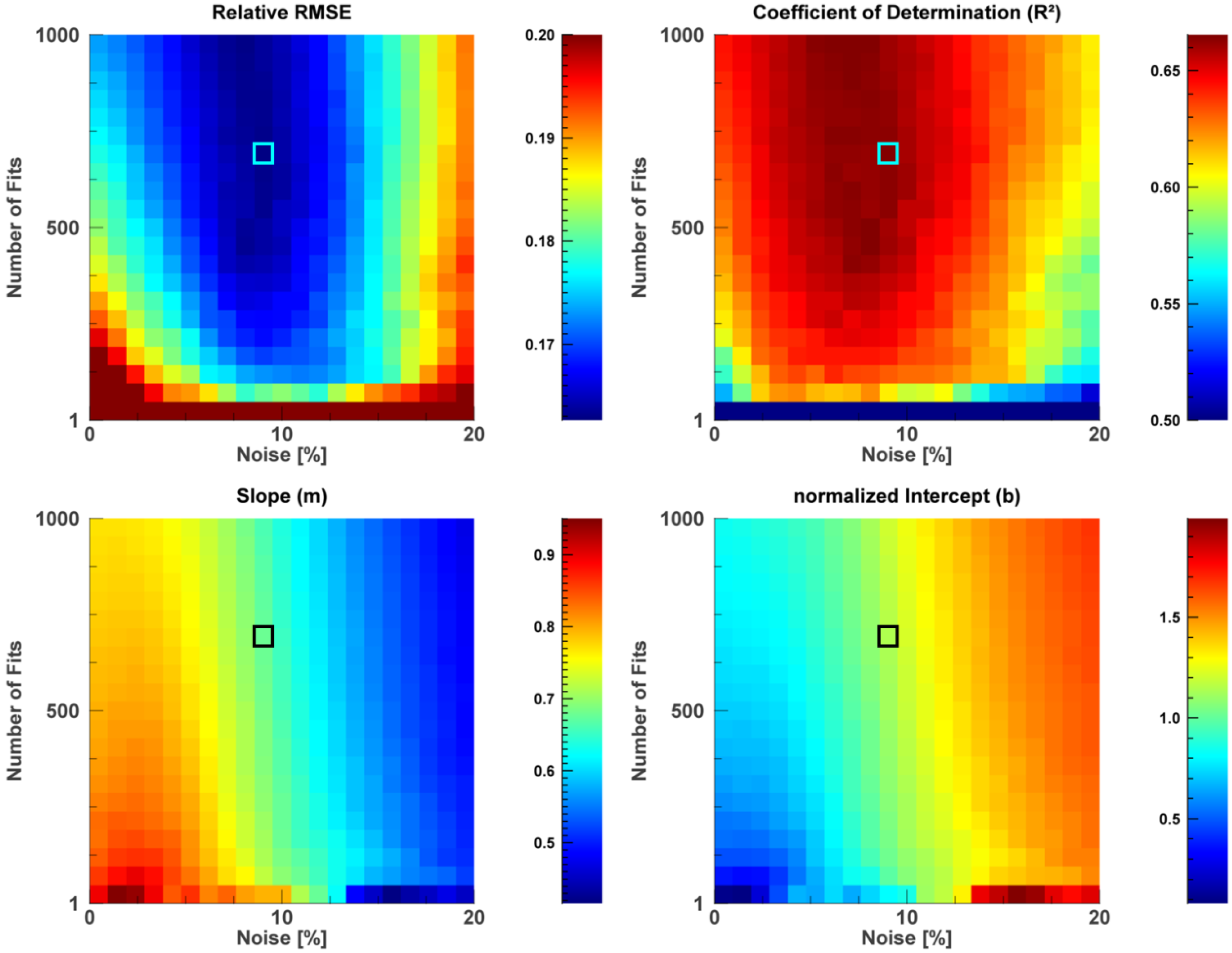
2.3. Selection Criteria

2.3.1. Band Selection

The first criterion is the selection of bands to be used for the comparison of the measured and simulated reflectance. Since the quality of reflectance data might differ among the available bands mostly due to noise, they must be selected wisely to avoid potentially corrupt results. Many studies (e.g., [34,35]) found that an appropriate band selection, or, alternatively, a specific weighting of different spectral bands, leads to an improvement in the inversion quality and prevents biases in the parameter estimation. Making an informed selection is, however, not trivial. A strategy to consider is the one proposed by Darvishzadeh et al. [25], who suggested discarding those wavelengths that are not well simulated by PROSAIL using an iterative approach, starting with the elimination of the worst modeled spectral band among all sample plots. The LUT inversion is repeated until all bands show acceptable accuracies within a user-specified threshold.

In view of the expected spectral capacity of EnMAP, which will provide spectrally contiguous data, a different approach was applied in this study by neglecting band selection apart from atmospherically distorted bands. This was based on the assumption that an applied curve fitting would be the more precise the more bands are considered and is related to the fact that the contiguous spectrum contains more information, e.g., on specific absorption ranges, than a multispectral dataset. Although the use of all available bands may provide redundant information when trying to retrieve individual parameters, e.g., LAI, this method has the advantage that some surface parameters, affecting reflectance in different and in some cases very small wavelength ranges, can be derived by a uniform method. Consequently, after excluding the bands located within the atmospheric water vapor absorption range and some bands with reduced sensitivity, located at the marginal areas of the CCDs, the remaining 146 bands were finally used in the inversion process.

2.3.2. Artificial Noise

A fundamental difference between simulated and measured reflectance, which was gathered by the use of airborne sensors, is the fact that the latter is affected by uncertainties originating from measurement inaccuracies and from the preprocessing steps of sensor calibration, geometric correction and radiometric calibration. On the other hand, the reflectance model might produce uncertainties as well, which are associated with its complex architecture for the calculation of canopy radiative transfer [33].

Compensating the uncertainties of both, sensor data and potential model weaknesses, is the reason for adding noise to the data. The type and amount of noise introduced differs in studies found in the literature. Bacour et al. [31], e.g., added 4% white Gaussian noise with no bias to the data. Baret et al. [32], by contrast, added white Gaussian noise to the reflectance values, which has an absolute value of 0.04. A combination of both with an additive level of 0.01 and a multiplicative level of 4% was used by Verger et al. [33]. In a study by Verrelst et al. [36], a systematic approach was pursued, which examined the effect of adding 0%–30% Gaussian noise to the data in 1% intervals. A modified approach was investigated by Rivera et al. [37] in which the influence of a multiplicative noise ranging from 0%–50%, in 2% intervals, was tested.

Comparable to the latter two studies, an approach combining different noise types was adopted to identify the noise level leading to the best possible results in this study. In this approach, both additive and multiplicative Gaussian noise as well as a combination of both was used. Of decisive importance for the amount of noise is the variance (σ²) in the Gaussian distribution [36].

Since the impact of multiplicative noise on the reflectance depends on the individual value of each band, high reflectance values, for example those occurring in the red edge, obtain higher noise values than low reflectances. However, low reflectance values are typically more prone to noise due to a lower light intensity reaching the sensor, which results in a lower signal-to-noise ratio (SNR) for the affected band. Therefore, an inverse form of multiplicative noise, having a stronger impact on low reflectance values than on high values, was tested as well. This is achieved by simply subtracting the simulated reflectance value at the given wavelengths, which can range from 0–1, from the highest possible reflectance value of 1. A total of five types of noise were defined for this study and tested concerning their performance. They are described by Equations (1)–(5):

Additive noise (Equation (1))

$$R_{ns}\left(\text{λ}\right)=R_{sim}\left(\text{λ}\right)+\chi \left(0,\text{σ}\left(\text{λ}\right)\right)$$

(1)

Multiplicative noise (Equation (2))

$$R_{ns}\left(\text{λ}\right)=R_{sim}\left(\text{λ}\right)\times \left[1+\chi \left(0,\text{σ}\left(\text{λ}\right)\right)\right]$$

(2)

Inverse-multiplicative noise (Equation (3))

$$R_{ns}\left(\text{λ}\right)=1-\left\{\left[1-R_{sim}\left(\text{λ}\right)\right]\times \left[1+\chi \left(0,\text{σ}\left(\text{λ}\right)\right)\right]\right\}$$

(3)

Combined noise (Equation (4))

$$R_{ns}\left(\text{λ}\right)=R_{sim}\left(\text{λ}\right)\times \left[1+\chi \left(0,2\text{σ}\left(\text{λ}\right)\right)\right]+\chi \left(0,\text{σ}\left(\text{λ}\right)\right)$$

(4)

Inverse-combined noise (Equation (5))

$$R_{ns}\left(\text{λ}\right)=1-\left\{\left[1-R_{sim}\left(\text{λ}\right)\right]\times \left[1+\chi \left(0,2\text{σ}\left(\text{λ}\right)\right)\right]\right\}+\chi \left(0,\text{σ}\left(\text{λ}\right)\right)$$

(5)

where

• $R_{ns}\left(\text{λ}\right)$ simulated reflectance value for band λ with noise
• $R_{sim}\left(\text{λ}\right)$ simulated reflectance value for band λ
• $\chi \left(0,\text{σ}\right)$ Gaussian distribution (mean value 0 and standard deviation σ)
• $\text{σ}\left(\text{λ}\right)$ uncertainties within the Gaussian distribution for band λ

In order to account for the fact that a given variance value has a less pronounced effect when applied as multiplicative noise, it is double-weighted compared to the additive noise factor in the combined methods.

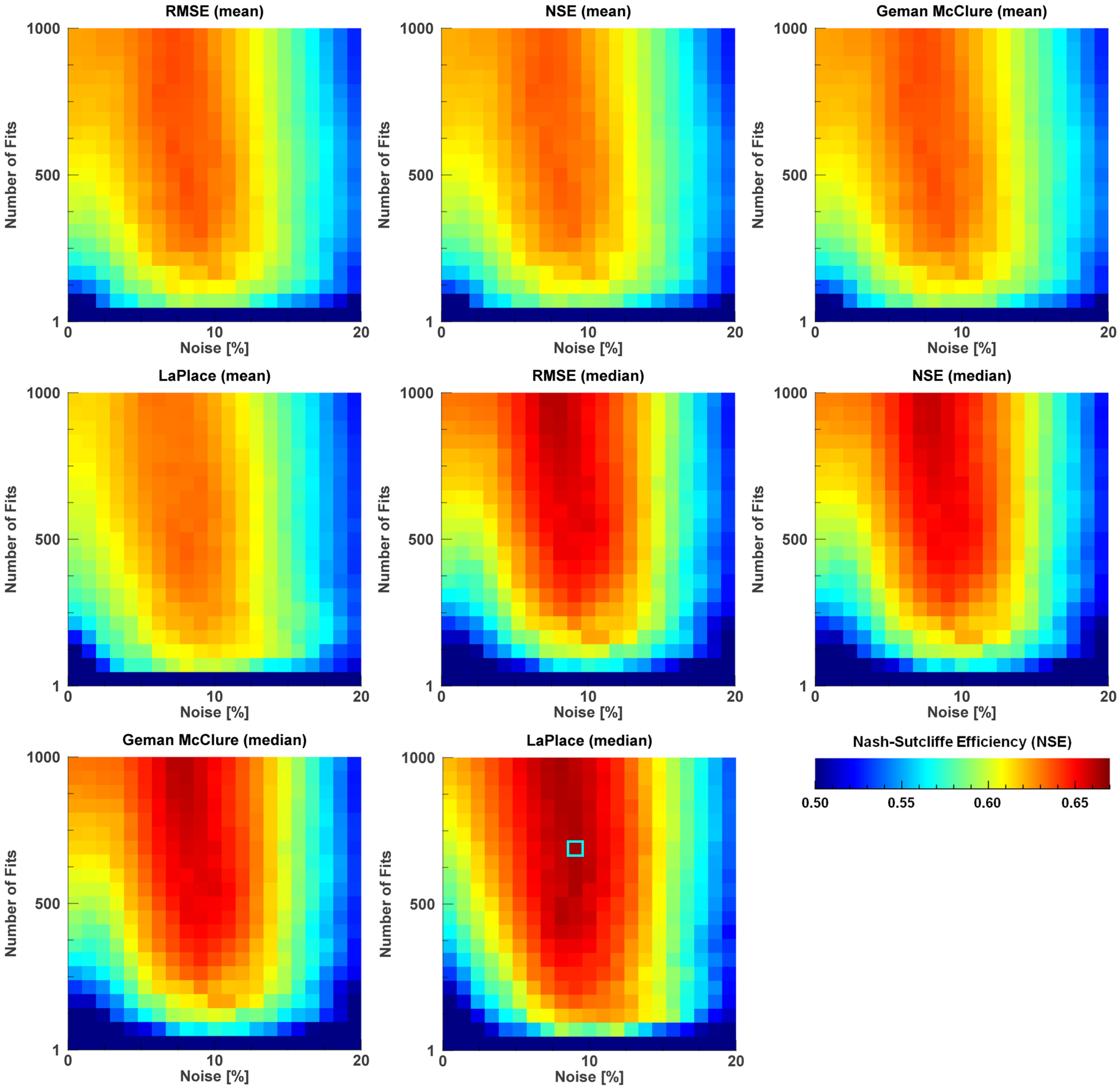
2.3.3. Cost Function

The cost function measures the discrepancies between observed and simulated reflectance values [13] and therefore serves for the purpose of identifying the combination by which the error between the simulated data provided by the LUT and the measured reflectance is minimized. Recently, several studies have investigated the potential of alternative cost functions for the retrieval of best fits between measured and simulated data (e.g., [36,37,38]). One of the most common measures in this context is the root mean square error (RMSE), which has been applied in several studies (e.g., [23,26,31]). For this reason, it was chosen as one of the cost functions applied in this study. The widely used least-square estimators (L2-means) produce good results, when the underlying assumptions, such as noise is Gaussian, are true [37]. Two further L2-estimators, i.e., Nash-Sutcliffe Efficiency (NSE) [39] and Geman & McClure Estimator (GM) [40], and a L1-estimator (absolute value), which is represented by the Laplace Distribution (LP) [40], were tested. The NSE is a measure of the mean square error to the observed variance, and is sensitive to large errors [39]. Among all cost functions, the very general Laplace Distribution represents the simplest one. This L1‑estimator calculates the distance, or, in other words, the area, between two spectra. As a result of its design, outlier values, which in general produce the largest errors, exert a less pronounced influence on the overall result when compared to the NSE. This advantage is also the case for the GM. However, this last measure cannot guarantee the identification of a unique best fit [37], which is a general requirement of a robust M-estimator. The cost functions are described by Equations (6)–(9). It is noted that in this study, both the RMSE and the NSE are not only used as a cost function, they also support model validation.

$$RMSE= \sqrt{\frac{1}{n}{\displaystyle \sum }_{\text{λ}=1}^n{\left(R_{msd}\left(\text{λ}\right)-R_{sim}\left(\text{λ}\right)\right)}^2}$$

(6)

$$NSE=1-\frac{{{\displaystyle \sum }}_{\text{λ}=1}^n{\left(R_{msd}\left(\text{λ}\right)-R_{sim}\left(\text{λ}\right)\right)}^2}{{{\displaystyle \sum }}_{\text{λ}=1}^n{\left(R_{msd}\left(\text{λ}\right)-{\overline{R}}_{msd}\right)}^2}$$

(7)

$$GM= {\displaystyle \sum }_{\text{λ}=1}^n\frac{{\left(R_{msd}\left(\text{λ}\right)-R_{sim}\left(\text{λ}\right)\right)}^2}{\left(1+{\left(R_{msd}\left(\text{λ}\right)-R_{sim}\left(\text{λ}\right)\right)}^2\right)}$$

(8)

$$LP= {\displaystyle \sum }_{\text{λ}=1}^n\left|R_{msd}\left(\text{λ}\right)-R_{sim}\left(\text{λ}\right)\right|$$

(9)

where

• $R_{msd}\left(\text{λ}\right)$ measured reflectance at band λ
• $R_{sim}\left(\text{λ}\right)$ simulated reflectance at band λ
• ${\overline{R}}_{msd}$ mean of measured reflectance among all bands

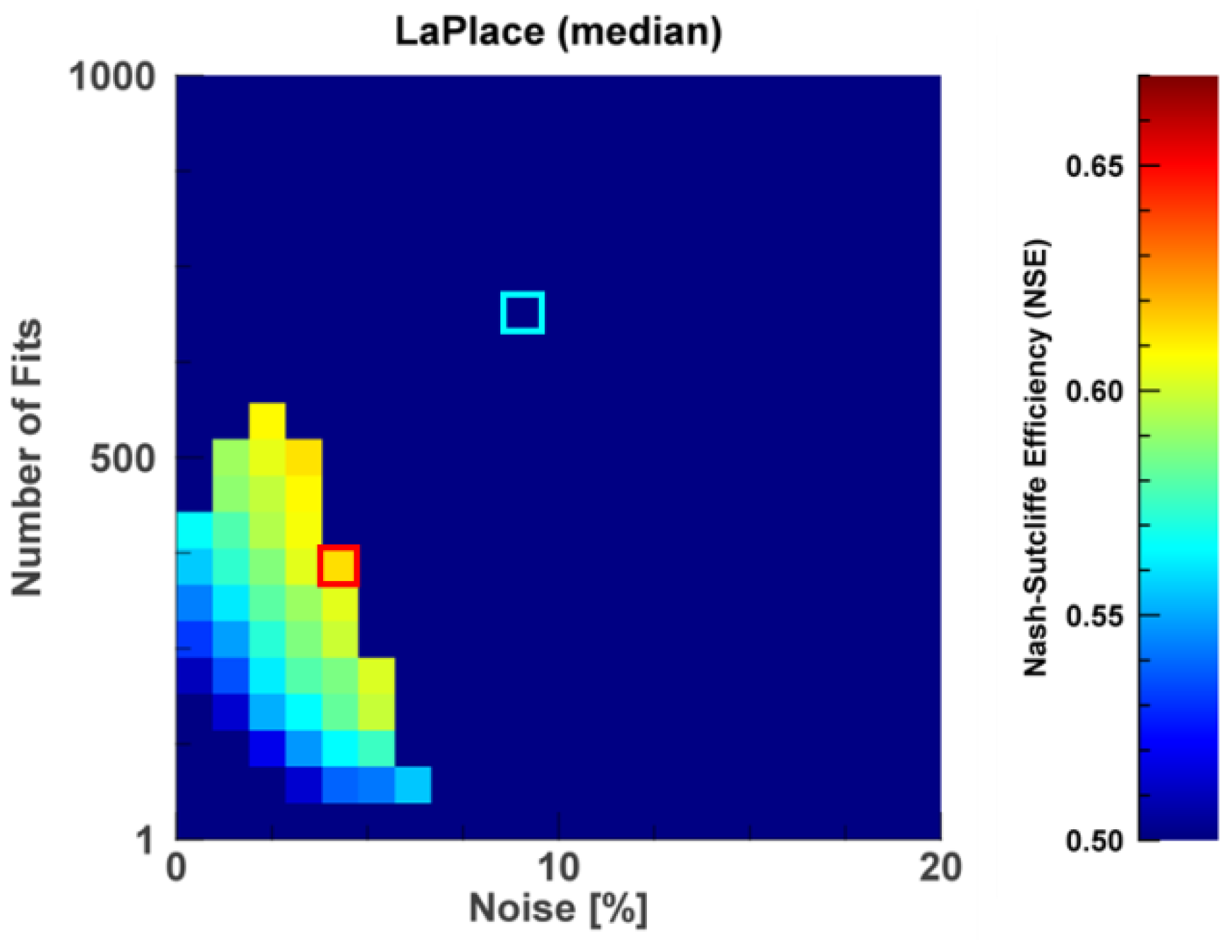
2.3.4. Ill-Posed Problem & Averaging Method

The ill-posed nature of inverting radiative transfer models is caused by the fact that different parameter settings can lead to the simulation of identical spectra. Many studies (e.g., [15,26,27,37]) have shown that the single best fit identified by the cost function does not necessarily lead to the best retrieval accuracy. This problem can be mitigated by taking a certain number of best fits between measured and modeled reflectance signatures into account, rather than just one single best fit. A threshold is defined based on the best fit determined by the cost function. Within the resulting range, each given input parameter is averaged. To define the threshold, Richter et al. [23] used the root mean square error (RMSE) as cost function and considered all combinations lying within the range of less than 10% of the lowest RMSE value.

Alternatively, a predefined number of best fits can be used instead of a percentage weighting, which was applied in this study, where various settings are tested. The consideration of a certain amount of best fits potentially mitigates the influence of misleading parameter configurations. In addition, the effect of averaging the corresponding input parameters of the resulting spectra selected from the LUT by both mean and median were examined. This was also investigated by Combal et al. [25], who tested the influence of the above mentioned averaging methods on the best 10 and 100 simulations, respectively.

In view of the multiple options and potential combinations of selection criteria, a strategy for the systematical examination of the best fit(s) has to be defined. This is a major goal of this study.

2.4. Design of Retrieval Procedure

The in-situ measurements of LAI served as reference, enabling validation by comparing the field measurements to the retrieved information of the corresponding pixels. In order to incorporate as many of the above listed selection criteria as possible, an inversion loop was implemented, which is described in the following.

To find the optimized amount of noise for each type, the variance of the Gaussian distribution describing the noise was set to 21 different levels, beginning with 0%, which means that no noise was added, up to a maximum of 5%, 10% or 20%, depending on the noise type. Various ranges were chosen to take the different weighting that variance has for each noise type into account. In the next step, all four cost functions (Equations (6)–(9)) were used to search for the best fit between the measured and the (noisy) simulated data. To find the best strategy for mitigating the ill-posed problem, a total of 21 steps considering a predetermined number of solutions incorporating multiple solutions (best fits) were defined and averaged. The first step represents only the overall best fit, the second solution represents the average of the best 50 fits. The incorporation of additional fits is continued with step sizes of 50 additional spectra per solution until the last step, the 21st, is reached, which then takes 1000 spectra, i.e., 1% of the complete LUT, into account. When averaged, both mean and median were used.

Since every possible combination of criteria within the defined range was calculated, the total number of single inversions is the product of different noise types (n = 5), various amounts of noise (n = 21), different cost functions (n = 4), number of best fits (n = 21) and the two separate averaging methods (n = 2). Consequently, a total of 17,640 singular inversions were conducted and each validated against the in-situ database of LAI.

3. Results

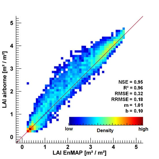
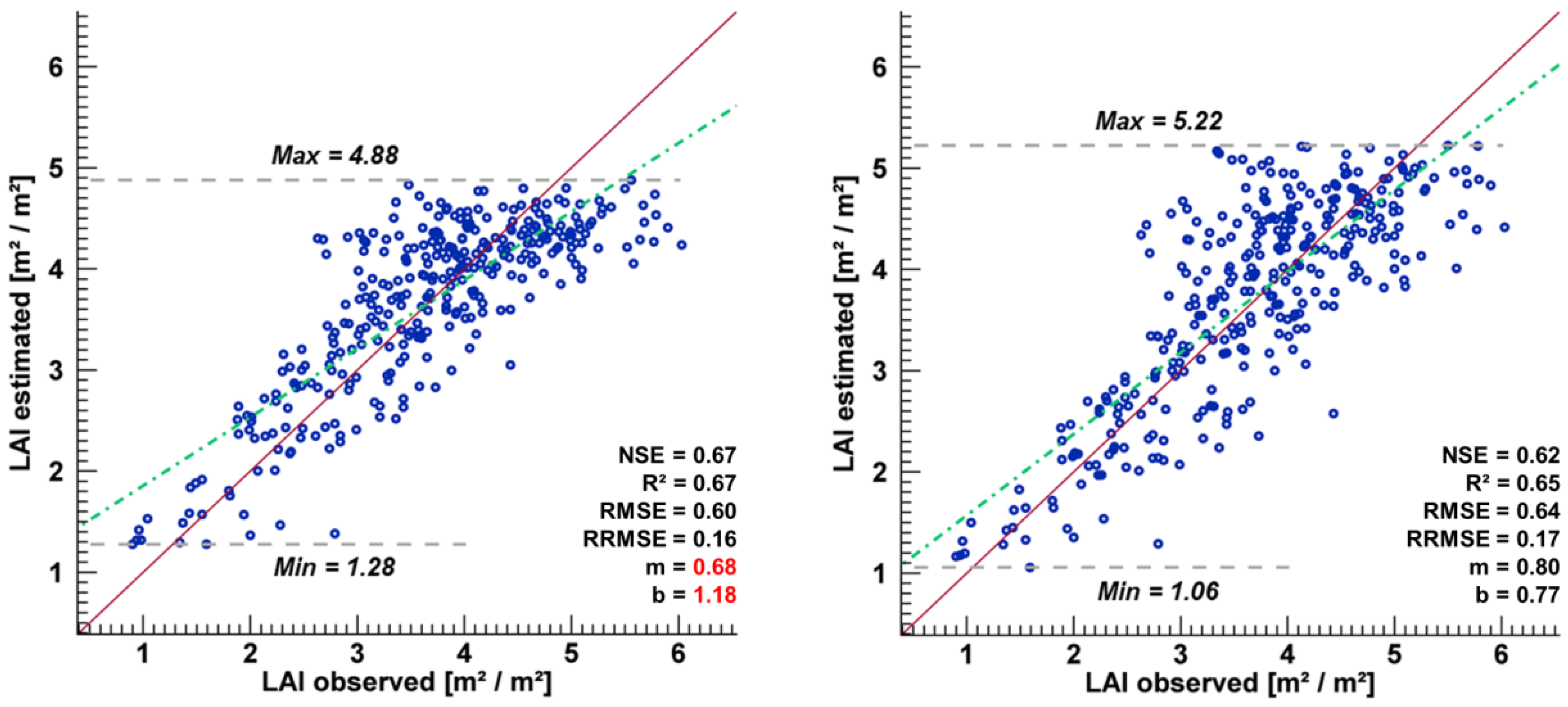
3.1. Validation of the Estimation Quality

The assessment of the inversion loop results led to the identification of an optimized configuration showing the highest accuracy of estimated parameters when compared to the observed in-situ measurements. It is noted that the method does not target optimization, but a validation of independent retrieval strategies. Due to its good applicability for assessing model prediction capabilities [39], the NSE was used as primary measure for the description of the estimation accuracy. Other measures were secondarily used to identify weaknesses in the data that are not described by the NSE. This was done due to the fact that the use of just one measure often insufficiently describes the model’s accuracy [41]. These measures are RMSE, coefficient of determination (R²), slope (m) and intercept (b) of Theil-Sen regression and relative RMSE (RRMSE). Figure 2 presents the result of the inversion loop for the inverse-multiplicative noise type, which turned out to perform best among all five noise types. The figure contains eight accuracy (NSE) matrices, representing the combinations of the four cost functions and two averaging methods. Each matrix contains 441 squares, giving the accuracy for every possible combination of the 21 settings of corresponding noise (σ) and the number of considered fits, which also have been tested in 21 settings. This style of presentation was chosen, since it was expected that the two selection criteria having the greatest influence would be the amount of noise, i.e., the standard deviation (σ), which was added to the simulated data, and the number of multiple solutions, i.e., best fits (n), which were considered and averaged for the parameter retrieval.

Figure 2. Accuracy matrices for the inverse-multiplicative noise type. The matrices are sorted by cost function/averaging method and show the estimation accuracy (NSE) for each combination of noise variance and number of considered best fits. The blue-marked square at the Laplace/median matrix represents the combination (σ = 9%, n = 700) with the highest accuracy among all possible combinations of selection criteria, including noise type.

Figure 2. Accuracy matrices for the inverse-multiplicative noise type. The matrices are sorted by cost function/averaging method and show the estimation accuracy (NSE) for each combination of noise variance and number of considered best fits. The blue-marked square at the Laplace/median matrix represents the combination (σ = 9%, n = 700) with the highest accuracy among all possible combinations of selection criteria, including noise type.

As indicated by Figure 2, several combinations of selection criteria result in NSE values of >0.5, indicating a good prediction accuracy of the model. It should be noted that for the purpose of contrast enhancement the range of the presented NSE values was set to be comparatively narrow (0.50−0.67, see legend of Figure 2), allowing for an intuitive interpretation of the results. The comparison of the eight matrices shows that they all feature similar patterns and that the ideal amount of noise is found between 7% and 12%. Concerning the number of fits, almost all matrices show an increasing accuracy with an increasing number of best fits included in the analysis.

Some matrices indicate that the highest accuracy values are achieved by the use of 1000 solutions and thus reach the boundary of the experiment. This leads to the question whether a higher number (>1000) than applied in this study would have led to even higher accuracies. The further evaluation presented in this section will, however, negate this theory. Due to the narrow range of displayed NSE values, which prohibits a differentiation of NSE values < 0.5, since these are, in Figure 2, all represented by the same dark blue color, it is not apparent which NSE values are reached when only the absolute best fit (n = 1) is used. In fact, NSE values < 0 occurred, regardless of the amount of noise applied to the data. This is directly attributed to the ill-posed problem and proves that a single fit potentially leads to completely misleading parameter retrieval.

The comparison of the influence of the different noise types revealed that there is no significant difference in the model accuracies. The best results were obtained by inverse-multiplicative noise (NSE = 0.67), followed by additive and inverse-combined noise (NSE = 0.66). Despite the fact that the classical multiplicative noise performs worst (NSE = 0.65), implying that the assumptions that led to the implementation of an inverse mode of this noise type were correct, the differences in the highest accuracy achieved by the different modes are too small to be of meaningful relevance.

The evaluation of the different cost functions revealed that they too led to similar estimation accuracies. However, a striking difference in accuracy was caused by the choice of the statistical method applied for the averaging of the simulated spectra, i.e., whether the mean or the median were used. Throughout all cost functions, the median provided higher accuracies. All in all, the cost function providing the best result (NSE = 0.67) is the Laplace distribution, based on 9% noise and averaging an amount of 700 solutions by the median. A possible explanation for the Laplace/median combination providing the highest accuracy among all possible combinations is the fact that the Laplace Distribution is a L1-estimator, which is less prone to outliers than the L2-estimators. Among these three combinations, the one based on inverse-multiplicative noise, a noise variance of 9% and a considered number of 700 fits, provides the best inversion method leading to the highest accuracy. This is valid at least when applying the NSE as validation estimator.

To evaluate this result in a wider range, Figure 3 shows the Laplace/median matrix of the inverse multiplicative noise, displayed as RRMSE, R², slope (m) and normalized intercept (b) instead of NSE. Since the values of intercept strongly depend on the absolute values of the data in general, a normalized version was generated by dividing it by the standard deviation of the in-situ data. This ensures comparability and provides a more accurate assessment. Since the RMSE shows behavior almost identical to the RRMSE, it is not included.

Figure 3. Alternative accuracy matrices (RRMSE, R², m, b) for the Laplace/median combination based on inverse-multiplicative noise, which has been identified as resulting in the highest accuracy based on the NSE. The marked square shows the position of the best solution selected by the NSE.

Figure 3. Alternative accuracy matrices (RRMSE, R², m, b) for the Laplace/median combination based on inverse-multiplicative noise, which has been identified as resulting in the highest accuracy based on the NSE. The marked square shows the position of the best solution selected by the NSE.

Figure 3 reveals that the different statistical indicators partially result in different patterns. The matrices of RRMSE and R² show a comparatively similar behavior to the NSE matrix of Figure 2, which almost confirms the position of the best fit. By contrast, slope and normalized intercept show a distinct deviation to the NSE pattern. Furthermore, the slope value of 0.68 lies far beyond the range of recommended values to indicate agreement [41]. As mentioned before, a divergent slope leads to an asymmetry between the observed and estimated data and therefore identifies the formerly determined best fit combination as inappropriate.

Taking this finding into account, a slope/intercept rejection threshold was defined. The threshold was applied to the accuracy estimation by the NSE and led to an exclusion of all combinations of selection criteria, where slope and intercept lay beyond the threshold. Following the recommendation of Richter et al. [41], the slope (m) rejection threshold is defined by: 0.8 ≤ m ≤ 1.2

Since intercept depends on the absolute values of the underlying data, a general threshold could not be defined. By contrast, a threshold for the normalized intercept is fully transferable; consequently the intercept (b) rejection threshold was set to: b ≤ 1.00

This combination of both thresholds means that all combinations based on a slope, which is lower than 0.8 or greater than 1.2, and based on an intercept, which exceeds 100% of the standard deviation of the observed data, are rejected. Figure 4 presents the NSE accuracy for the Laplace/median combination based on inverse-multiplicative noise, after the slope/intercept rejection threshold was applied. All accuracies that are rejected due to the thresholds were excluded and were set to zero.

Figure 4. Accuracy matrix for the Laplace/median combination based on inverse-multiplicative noise after the rejection threshold for slope (0.8 ≤ m ≤ 1.2) and intercept (≤1.00) was applied. The red-marked square shows the combination with the highest accuracy (σ = 4%, n = 350), which resulted in a value for NSE of 0.62 after the exclusion of inappropriate combinations due to the thresholds. For comparison, the blue-marked square shows the position of the formerly identified ideal criteria combination, which had been derived without taking slope and intercept of the regression into account.

Figure 4. Accuracy matrix for the Laplace/median combination based on inverse-multiplicative noise after the rejection threshold for slope (0.8 ≤ m ≤ 1.2) and intercept (≤1.00) was applied. The red-marked square shows the combination with the highest accuracy (σ = 4%, n = 350), which resulted in a value for NSE of 0.62 after the exclusion of inappropriate combinations due to the thresholds. For comparison, the blue-marked square shows the position of the formerly identified ideal criteria combination, which had been derived without taking slope and intercept of the regression into account.

After applying the rejection thresholds to the data, the Laplace/median matrix has distinctly changed in appearance. All higher noise levels (above 7%) as well as the higher numbers of considered solutions (>550) have been rejected. Compared to the other matrices of the inverse-multiplicative noise type, which are not shown in Figure 4, the median is still stronger than the mean among all cost functions. For the Laplace/median matrix, the best solution has moved to the bottom left, indicating a lower noise level and a reduced number of considered best fits compared to the former combination with the highest accuracy according to NSE. The new solution provides the best result with NSE = 0.62, which still is a strong indication of good model performance (>0.5), and is based on 4% noise and on the averaging of 350 solutions by the median.

To illustrate the impact of the modification, and in order to examine whether the statistical measures provide valid values, Figure 5 shows the scatter plots of the LAI estimation based on the best LUT selection criteria combination before and after the slope/intercept rejection threshold was applied.

Although NSE, R², RMSE and RRMSE provided higher accuracies in the original LUT setting, the scatter plot (Figure 5, left) shows an asymmetry which is distinctly reduced after the application of the rejection threshold (Figure 5, right). It is assumed that the asymmetry, which is visible through a high minimum and a low maximum value in the estimated data, originated from the input parameter setting of the LUT following a Gaussian distribution. Since most LAI values of the input data scatter around values >2.0 and <5.0, a consideration of a high number of solutions leads to strong generalization and consequently to a loss of information. This is due to the fact that, in addition to the LUT spectra that are based on matching LAI information, a high number of other spectra are considered, which are based on input parameters with the most common LAI values, i.e., >2.0 and <5.0. The amount of noise might have an influence as well, since all combinations based on values >5% were also rejected.

Figure 5. Correlation of observed and estimated LAI. (Left) The scatter plot is based on the LUT criteria setting (Laplace/median, n = 700, σ = 9%, inverse-multiplicative noise), which resulted in the highest accuracy according to NSE; (Right) The scatter plot is based on the highest accuracy after applying the slope/intercept rejection threshold (n = 350, σ = 4%).

Figure 5. Correlation of observed and estimated LAI. (Left) The scatter plot is based on the LUT criteria setting (Laplace/median, n = 700, σ = 9%, inverse-multiplicative noise), which resulted in the highest accuracy according to NSE; (Right) The scatter plot is based on the highest accuracy after applying the slope/intercept rejection threshold (n = 350, σ = 4%).

Consequently, the scatter plot incorporating the rejection threshold has a more common appearance, since it is not as clinched. The now adequate values of slope and intercept involved a slight deterioration of the other quality measures, which nonetheless are still at acceptable levels.

Based on the estimated vegetation parameters, the progressing development of specific crops throughout the growing season could be analyzed. Figure 6 shows the development of LAI for the investigated crops from 28 April to 8 September. The information was extracted from the retrieved parameter products by randomly choosing and averaging 30 pixels per scene and each crop type from the corresponding parameter.

Figure 6. Seasonal development of LAI for the five investigated crops throughout the growing period of 2012, derived from six data acquisitions.

Figure 6. Seasonal development of LAI for the five investigated crops throughout the growing period of 2012, derived from six data acquisitions.

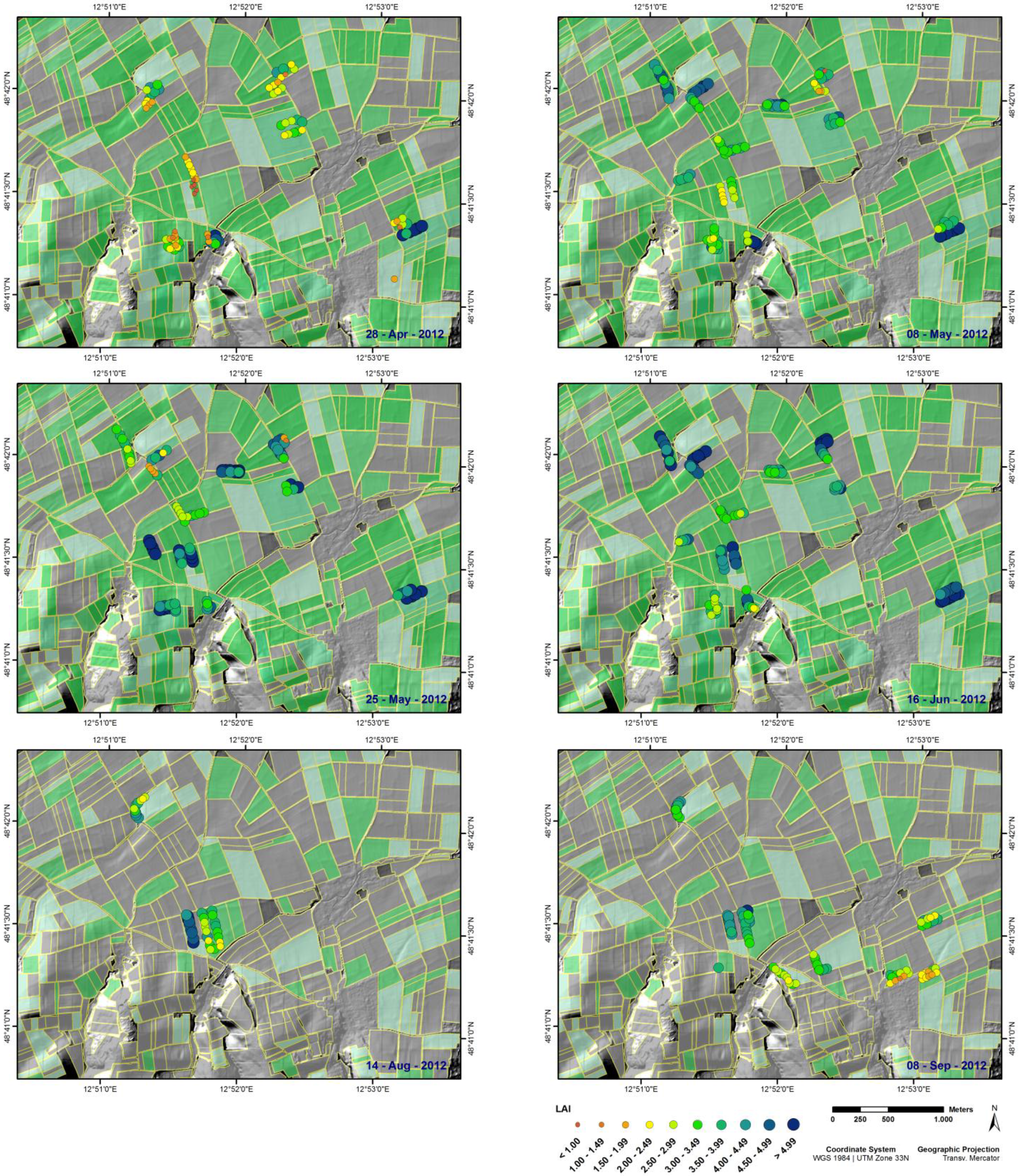
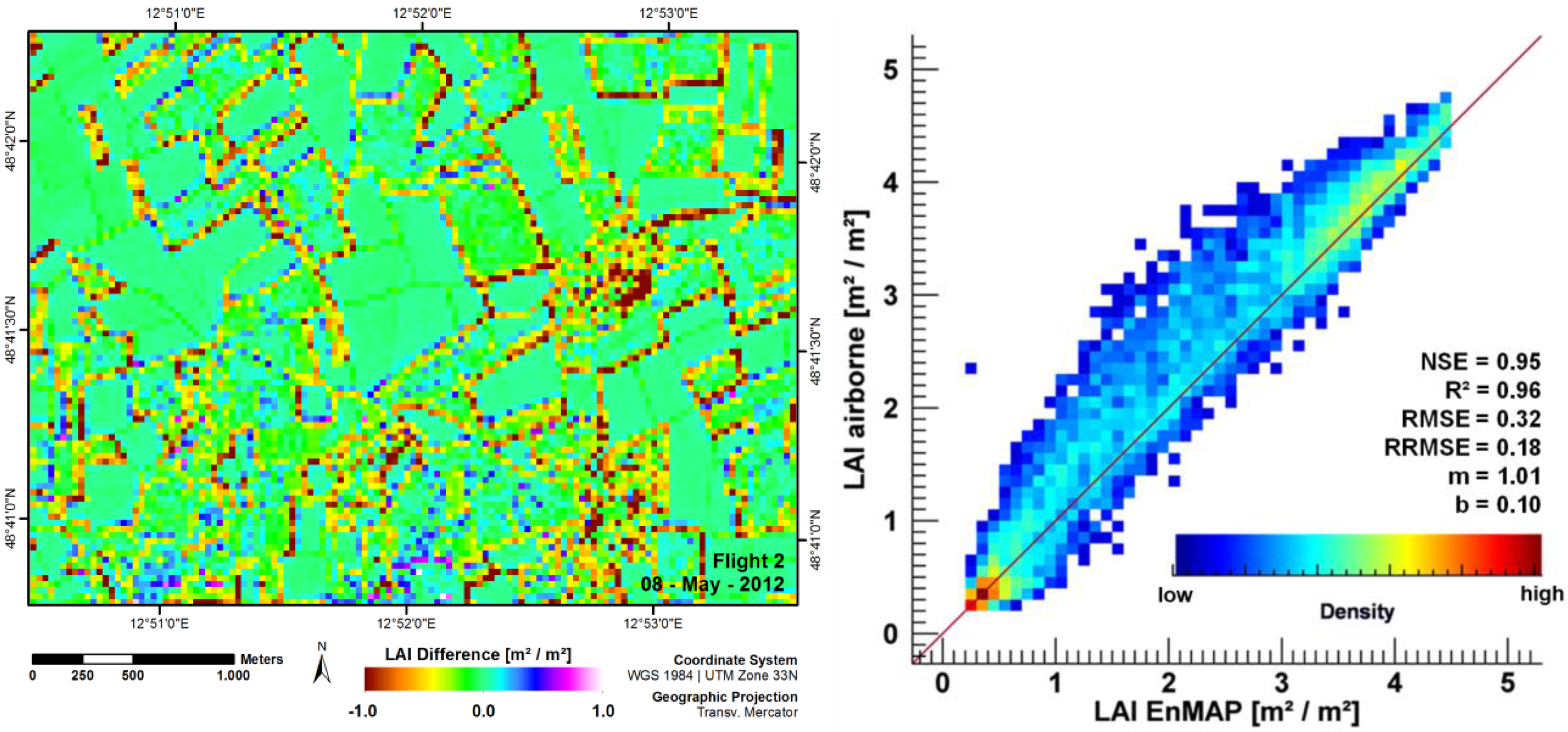
3.2. Transferability to the EnMAP Scale

In order to evaluate the capacity of the analysis method for the retrieval of LAI from future EnMAP data, the LUT inversion was adapted and repeated on the simulated EnMAP data, based on the identical setting as it had been used for the airborne data. The application of the inversion method to the simulated EnMAP data requires validation as well. This, however, is not easily done based on in-situ measurements, since ground measurements naturally only are representative for the spatial resolution for which they were collected. In our case, the LAI data was sampled at a diagonal sampling pattern within ESUs of 4 by 4 m and thus correspond to the 4 m scale of the airborne data. EnMAP, however, will operate at a geometric resolution of 30 m, making it very hard to acquire statistically significant amounts of overpass-parallel in-situ measurements for ESUs of that considerable spatial extent. Consequently, another approach was chosen, which uses the results of the parameter retrieval based on the airborne image data. Since the estimation accuracy on the 4 m scale of the airborne acquisitions was proved to be acceptable by validation against in-situ data, the validated output images were scaled up to the spatial resolution of 30 m, thus generating a validated spatial LAI map at 30 m resolution. This validated map then was consulted as reference for the LAI map that was originally retrieved from the simulated EnMAP data at 30 m resolution. The acquisition of the second flight on 8 May 2012 was used for the comparison. In Figure 7, the LAI image retrieved from the simulated EnMAP scene and the upscaled airborne LAI map are presented.

Figure 7. Comparison of estimated LAI (8 May 2012), which was derived by the adapted LUT algorithm from simulated EnMAP data (Left) and upscaled (from 4–30 m) LAI estimation based on the 4 m airborne data (Right).

Figure 7. Comparison of estimated LAI (8 May 2012), which was derived by the adapted LUT algorithm from simulated EnMAP data (Left) and upscaled (from 4–30 m) LAI estimation based on the 4 m airborne data (Right).

The visual interpretation of Figure 7 shows that the estimations of LAI appear to have led to very similar results in both maps. To further assess the consistency between airborne and EnMAP retrieval, an uncertainty map of both scales is presented in Figure 8, giving the standard deviation of all considered estimated LAI values (n = 350) per pixel before averaging. The maps, one for the airborne and one for the EnMAP-scale retrieval, give a spatial measure of how definite the resulting LAI value was found among the simulated spectra that were selected by the inversion routine. By comparing Figure 7 and Figure 8, it can be observed that high LAI values are generally associated with higher uncertainty. The highest levels of uncertainty are observed for the forested areas in the South of the test area. This can to some degree be traced to the fact that the parameters included in the LUT were not designed to include characteristics of forested areas, because forests were not targeted in this study. For both scales, the standard deviation among the 350 best fits is roughly 1 LAI unit. However, it also can be deduced that the model uncertainty on average increases by 3% when going from the airborne (Figure 8, right) to the satellite borne scale (Figure 8, left).

Figure 8. Standard deviation of all considered estimated LAI values (n = 350) before averaging, giving a spatial measure of model uncertainty for the retrieval of LAI from simulated EnMAP data (Left) and from airborne data (Right).

Figure 8. Standard deviation of all considered estimated LAI values (n = 350) before averaging, giving a spatial measure of model uncertainty for the retrieval of LAI from simulated EnMAP data (Left) and from airborne data (Right).

In order to examine local deviations and to determine whether they follow a spatial pattern, a map was calculated showing the difference between the simulated EnMAP and the upscaled airborne estimation (Figure 9, left). Further, the agreement between both spatial data sets was calculated by confronting each pixel of the LAI-EnMAP map to the corresponding one of the airborne scale LAI map (Figure 9, right).

The analysis shows that a very strong agreement exists, as evidenced by the consistently high values of the statistical indicators. Further, most pixels cluster along the diagonal of the density plot as well as around low and high LAI values, respectively (Figure 9, right). However, Figure 9 also shows that strong differences occur particularly in the marginal areas of fields, but also along streets and within developed areas such as villages. In these places, the LAI estimation based on airborne data generated almost consistently higher values than the one conducted using the simulated EnMAP data. This can be explained by uncertainties arising from differences in the incorporation of land surface heterogeneities in the two images, resulting from the different methods by which the two underlying datasets were generated. While the LAI-EnMAP estimation was performed on a simulated dataset, which had been spectrally and spatially resampled prior to the LUT inversion, the LAI-airborne map was created based on the original dataset and was spatially resampled to 30 m after the inversion process was finished. This means that, in the simulated EnMAP scene, small-scale heterogeneities had already been compensated for through the spectral redistribution of the nearly 200 reflectance values and the spatial upscaling of the image before the actual parameter retrieval was performed, which explains why the LAI values in these areas are lower. The parameter retrieval conducted at the 4 m airborne scale, however, explicitly took these spatial heterogeneities into account. When the latter was scaled-up afterwards, already existing extreme LAI values in the 4 m image had a stronger influence on the corresponding 30 m pixels compared to the estimation based on the up-scaled reflectance value in the simulated EnMAP scene. Conversely, this means that for homogenous areas this kind of scaling problem is barely existent. Figure 9 shows that this assumption is correct, as hardly any deviation can be determined within the fields themselves.

Figure 9. Difference map calculated from the LAI estimations based on simulated EnMAP and upscaled original airborne data (Left) and density plot showing a pixel-wise comparison of both spatial data sets (Right).

Figure 9. Difference map calculated from the LAI estimations based on simulated EnMAP and upscaled original airborne data (Left) and density plot showing a pixel-wise comparison of both spatial data sets (Right).

4. Discussion

Based on data from an extensive field campaign, the validation proved that the LUT approach provides a robust and transparent method for parameter estimation from hyperspectral data, without requiring the use of in-situ data. However, the specification of the different selection criteria on which the LUT setting can be based has to be thoroughly considered. In the past, many studies investigated the influence of various selection criteria. Nevertheless, the combined assessment of all criteria presented in our study has not been investigated systematically before. Some studies focused the influence of an appropriate band selection for the retrieval [25,34,35], others analyzed the potential of adding artificial noise to the data in an additive [32], multiplicative [31,36,37] or a combined form [33]. Besides the very well approved RMSE [23,26,31], alternative cost functions have been subject of various studies [36,37,38]. To counteract the influence of the ill-posed problem, the use of a multiple number of best fits is widely accepted [15,26,27,37], yet investigations of the averaging method are still rare, like the one from Darvishzadeh et al. [25], who analyzed the potential of mean and median.

Our study demonstrates that a systematic analysis of all those different selection criteria helps to examine their impact to the estimation quality and, if carefully selected, to increase the quality eventually.

The analysis of artificial noise led to the realization that it is not of decisive importance which type of noise is added to the simulated reflectances, but more so that some type of noise is added at all. Both, inverse-multiplicative and inverse-combined noise provided slightly more robust results. Another selection criterion resulting in only minor quality differences was the choice of the cost function. As a matter of fact, the mathematically simplest function, represented by the Laplace Distribution, performed best, possibly due to its lower susceptibility to outliers. Due to the slight differences in performance, an unambiguous definition of an ideal cost function is, nevertheless, not possible.

By contrast, the integration of a number of multiple solutions, the averaging method, and the amount of noise added to the spectra were identified to exert a major impact on estimation quality. The consideration of a multiple number of solutions proved to be an efficient way to handle the ill-posed problem. The use of the median rather than the mean as averaging method for the parameter combinations thus retrieved was clearly advantageous. This is attributable to the fact that the median is potentially less sensitive to outliers compared to the mean. This means that extreme values in a dataset exert a strong influence on the mean, while the median might not be affected at all, because the absolute values of extreme data points do not influence the median. When analyzing all accuracy matrices among all noise types, it turned out that in 17 out of 20 cases the median was stronger. Further, it was found that adding noise to the simulated data, regardless of the noise type, allows for a more flexible identification of spectra and their corresponding input parameter setting, which was evidenced by distinctly higher accuracies.

The use of a coordinated set of various statistical measures, as it is recommended by Richter et al. [41], supported the specification of the selection criteria. In consequence, it could be proved that the amount of noise and the number of solutions should both not be set too high, since this would lead to a sort of dilution. Especially when basing the input parameters on a Gaussian distribution, as it was the case in this study, this would soften the potential of such a distribution aiming at the precise differentiation of parameter values.

In view of the future EnMAP-HSI, it was shown that using the full potential of all available spectral bands for the inversion contributed to the achievement of robust estimation accuracies for leaf area index, even without applying parameter constraints. Thereby, the same retrieval method was applied at two scales that differed in their spatial, spectral and radiometric properties with similar accuracies. Due to the reduced radiometric and spectral quality of the satellite data in comparison to the airborne data, retrieval uncertainty was higher for the satellite-based retrieval by 3%. It seems natural that the overall accuracies achieved by this generalized approach are somewhat lower compared to studies that explicitly take prior information, such as land use or phenological status, into account (e.g., [23,26,27]).

5. Conclusions

EnMAP will supply >200 spectral bands for a contiguous high-quality representation of surface reflectance. The future satellite mission thus will enable a hyperspectral observation of biophysical variables at the Earth’s surface. Based on our assessment, this will enable an accurate analysis of the seasonal development of biophysical variables on the regional scale. By applying transferable physically based retrieval methods, such as the one used in this study, which was proved to be consistent and robust for the estimation of leaf area index without using prior information, the full potential of a spaceborne imaging spectrometer for vegetation studies can be utilized.

In order to validate the estimation accuracy for leaf area index from hyperspectral measurements, the outputs of different strategies to derive leaf area index from the PROSAIL model via LUT inversion in this study were compared to in-situ data using a set of statistical measures. This enabled the identification of potential weaknesses in the retrieval strategy. It was found that good results were achieved (NSE = 0.62, R² = 0.65, RMSE = 0.64, RRMSE = 0.17, m = 0.80 and b = 0.77) applying the following strategy: (i) by using the Laplace Distribution as cost function; (ii) by adding an inverse-multiplicative noise type; (iii) by adjusting the noise level to σ = 4%; (iv) by averaging the best 350 out of 100,000 fits from the LUT and (v) by using the median as the averaging method. It was also found that the impact of noise level, averaging method and number of considered best fits on the retrieval quality was high, while the impact of noise type and cost function was low.

In a following step, the LUT inversion was adapted to the spectral bands of the future EnMAP satellite and the modified LUT was applied in an inversion approach based on simulated EnMAP data. The results obtained from the simulated satellite data were validated against upscaled results of the airborne LAI estimation. By evaluating the conformity of the two LAI data sets acquired on different scales (NSE = 0.95, R² = 0.96, RMSE = 0.32, RRMSE = 0.18, m = 1.01 and b = 0.10), it was shown that the determined analysis method can successfully be applied to data constructed according to the radiometric, spectral and spatial characteristics of the upcoming EnMAP Hyperspectral Imager. Due to the lower radiometric and spectral quality of the satellite-based measurements compared to the airborne acquisitions, the model uncertainty was increased by 3% for the simulated satellite data. Taking this increased uncertainty into account, the proposed method will be applicable to real EnMAP data.

Nonetheless, due to the limited data base available for this study, the knowledge gained on the influence of the different selection criteria and the transferability of the method to the EnMAP scale in essence is restricted to the five crops that were analyzed (winter wheat, winter barley, maize, sugar beet, rapeseed) and to the land surface conditions found in Southern Germany. It is important to say that the identified strategy must not necessarily be valid for all types of sensors, crops and conditions. Since resources for field campaigns are limited, it can only be stated that the presented method works for the investigated crops. However, due to its generic nature, the method should be applicable to crops in general.

The important result of this study therefore is not a recommendation of fixed settings for an optimized retrieval of LAI, but rather an increase of knowledge about the influence of the different selection criteria. The findings of this study therefore should be confirmed through future studies, focusing on other/additional crops and ideally real EnMAP data obtained in other regions in order to test the acquired procedure also for geographic transferability, which has not been done in the context of this study. With EnMAP, the generation of seasonal series of hyperspectral data will become much easier compared to the efforts that were necessary to construct the data series used in this study from airborne campaigns. By conducting seasonal studies with the help of satellite-based hyperspectral data, the understanding of both, the PROSAIL model as well as the LUT inversion technique, can be further deepened.

References

1. Van Ittersum, M.K.; Cassman, K.G.; Grassini, P.; Wolf, J.; Tittonell, P.; Hochman, Z. Yield gap analysis with local to global relevance—A review. Field Crops Res. 2013, 143, 4–17. [Google Scholar] [CrossRef]
2. Kaufmann, H.; Förster, S.; Wulf, H.; Segl, K.; Guanter, L.; Bochow, M.; Heiden, U.; Mueller, A.; Heldens, W.; Schneiderhan, T.; et al. Science Plan of the Environmental Mapping and Analysis Program (EnMAP); Deutsches GeoForschungsZentrum GFZ: Potsdam, Germany, 2012; p. 63. [Google Scholar]
3. Govender, M.; Chetty, K.; Bulcock, H. A review of hyperspectral remote sensing and its application in vegetation and water resource studies. Water SA 2007, 33. [Google Scholar] [CrossRef]
4. Guanter, L.; Kaufmann, H.; Segl, K.; Foerster, S.; Rogass, C.; Chabrillat, S.; Kuester, T.; Hollstein, A.; Rossner, G.; Chlebek, C.; et al. The EnMAP spaceborne imaging spectroscopy mission for earth observation. Remote Sens. 2015, 7, 8830–8857. [Google Scholar] [CrossRef]
5. Duveiller, G.; Weiss, M.; Baret, F.; Defourny, P. Retrieving wheat green area index during the growing season from optical time series measurements based on neural network radiative transfer inversion. Remote Sens. Environ. 2011, 115, 887–896. [Google Scholar] [CrossRef]
6. Si, Y.; Schlerf, M.; Zurita-Milla, R.; Skidmore, A.; Wang, T. Mapping spatio-temporal variation of grassland quantity and quality using MERIS data and the prosail model. Remote Sens. Environ. 2012, 121, 415–425. [Google Scholar] [CrossRef]
7. Le Maire, G.; Marsden, C.; Verhoef, W.; Ponzoni, F.J.; Seen, D.L.; Bégué, A.; Stape, J.L.; Nouvellon, Y. Leaf area index estimation with MODIS reflectance time series and model inversion during full rotations of eucalyptus plantations. Remote Sens. Environ. 2011, 115, 586–599. [Google Scholar] [CrossRef]
8. Richter, K.; Vuolo, F.; D’Urso, G.; Dini, L. Evaluation of different methods for the retrieval of LAI using high resolution airborne data. Proc. SPIE Remote Sens. Agric. Ecosyst. Hydrol. IX 2007. [Google Scholar] [CrossRef]
9. Stevens, A.; Udelhoven, T.; Denis, A.; Tychon, B.; Lioy, R.; Hoffmann, L.; van Wesemael, B. Measuring soil organic carbon in croplands at regional scale using airborne imaging spectroscopy. Geoderma 2010, 158, 32–45. [Google Scholar] [CrossRef]
10. Oppelt, N.; Mauser, W. Hyperspectral monitoring of physiological parameters of wheat during a vegetation period using AVIS data. Int. J. Remote. Sens. 2004, 25, 145–159. [Google Scholar] [CrossRef]
11. Weiss, M.; Troufleau, D.; Baret, F.; Chauki, H.; Prévot, L.; Olioso, A.; Bruguier, N.; Brisson, N. Coupling canopy functioning and radiative transfer models for remote sensing data assimilation. Agric. For. Meteorol. 2001, 108, 113–128. [Google Scholar] [CrossRef]
12. Hank, T.; Bach, H.; Mauser, W. Using a remote sening-supported hydro-agroecological model for field-scale simulation of heterogeneous crop growth and yield: Application for wheat in central europe. Remote Sens. 2015, 7, 3934–3965. [Google Scholar] [CrossRef]
13. Jacquemoud, S.; Verhoef, W.; Baret, F.; Bacour, C.; Zarco-Tejada, P.J.; Asner, G.P.; Francois, C.; Ustin, S.L. PROSPECT plus SAIL models: A review of use for vegetation characterization. Remote Sens. Environ. 2009, 113, S56–S66. [Google Scholar] [CrossRef]
14. Jacquemoud, S.; Baret, F.; Andrieu, B.; Danson, F.M.; Jaggard, K. Extraction of vegetation biophysical parameters by inversion of the PROSPECT + SAIL models on sugar beet canopy reflectance data. Application to TM and AVIRS sensors. Remote Sens. Environ. 1995, 52, 163–172. [Google Scholar] [CrossRef]
15. Darvishzadeh, R.; Skidmore, A.; Schlerf, M.; Atzberger, C. Inversion of a radiative transfer model for estimating vegetation LAI and chlorophyll in a heterogeneous grassland. Remote Sens. Environ. 2008, 112, 2592–2604. [Google Scholar] [CrossRef]
16. Baret, F.; Buis, S. Estimating canopy characteristics from remote sensing observations: Review of methods and associated problems. In Advances in Land Remote Sensing; Springer: Dordrecht, The Netherlands, 2008; pp. 173–201. [Google Scholar]
17. Jacquemoud, S.; Bacour, C.; Poilvé, H.; Frangi, J.P. Comparison of four radiative transfer models to simulate plant canopies reflectance: Direct and inverse mode. Remote Sens. Environ. 2000, 74, 471–481. [Google Scholar] [CrossRef]
18. Verhoef, W.; Bach, H. Simulation of hyperspectral and directional radiance images using coupled biophysical and atmospheric radiative transfer models. Remote Sens. Environ. 2003, 87, 23–41. [Google Scholar] [CrossRef]
19. Oppelt, N.; Mauser, W. Airborne visible/infrared imaging spectrometer AVIS: Design, characterization and calibration. Sensors 2007, 7, 1934–1953. [Google Scholar] [CrossRef] [Green Version]
20. Baumgartner, A.; Gege, P.; Köhler, C.; Lenhard, K.; Schwarzmaier, T. Characterisation methods for the hyperspectral sensor HySpex at DLR’s calibration home base. Proc. SPIE Remote Sens. Agric. Ecosyst. Hydrol. XVI 2012. [Google Scholar] [CrossRef]
21. Richter, R.; Schläpfer, D. Atmospheric/Topographic Correction for Airborne Imagery, ATCOR-4 User Guide, Version 4.2; DLR: Wessling, Germany, 2007; p. 125. [Google Scholar]
22. Segl, K.; Guanter, L.; Rogass, C.; Kuester, T.; Roessner, S.; Kaufmann, H.; Sang, B.; Mogulsky, V.; Hofer, S. Eetes—The EnMAP end-to-end simulation tool. IEEE J. Sel. Top. Appl. Earth Obs. Remote Sens. 2012, 5, 522–530. [Google Scholar] [CrossRef]
23. Richter, K.; Atzberger, C.; Vuolo, F.; Weihs, P.; D’Urso, G. Experimental assessment of the Sentinel–2 band setting for RTM–based LAI retrieval of sugar beet and maize. Can. J. Remote Sens. 2009, 35, 230–247. [Google Scholar] [CrossRef]
24. Kimes, D.S.; Knyazikhin, Y.; Privette, J.L.; Abuelgasim, A.A.; Gao, F. Inversion methods for physically‐based models. Remote Sens. Rev. 2000, 18, 381–439. [Google Scholar] [CrossRef]
25. Darvishzadeh, R.; Atzberger, C.; Skidmore, A.; Schlerf, M. Mapping grassland leaf area index with airborne hyperspectral imagery: A comparison study of statistical approaches and inversion of radiative transfer models. ISPRS J. Photogramm. 2011, 66, 894–906. [Google Scholar] [CrossRef]
26. Combal, B.; Baret, F.; Weiss, M.; Trubuil, A.; Macé, D.; Pragnère, A.; Myneni, R.; Knyazikhin, Y.; Wang, L. Retrieval of canopy biophysical variables from bidirectional reflectance: Using prior information to solve the ill-posed inverse problem. Remote Sens. Environ. 2003, 84, 1–15. [Google Scholar] [CrossRef]
27. Vuolo, F.; Atzberger, C.; Richter, K.; D’Urso, G.; Dash, J. Retrieval of biophysical vegetation products from rapideye imagery. Proc. ISPRS Tech. Comm. VII Symp. -100 Years ISPRS -Adv. Remote Sens. Sci. 2010, XXXVIII, 281–286. [Google Scholar]
28. Durbha, S.S.; King, R.L.; Younan, N.H. Support vector machines regression for retrieval of leaf area index from multiangle imaging spectroradiometer. Remote Sens. Environ. 2007, 107, 348–361. [Google Scholar] [CrossRef]
29. Darvishzadeh, R.; Matkan, A.A.; Ahangar, A.D. Inversion of a radiative transfer model for estimation of rice canopy chlorophyll content using a lookup-table approach. IEEE J. Sel. Top. Appl. Earth Obs. Remote Sens. 2012, 5, 1222–1230. [Google Scholar] [CrossRef]
30. Weiss, M.; Baret, F.; Myneni, R.B.; Pragnère, A.; Knyazikhin, Y. Investigation of a model inversion technique to estimate canopy biophysical variables from spectral and directional reflectance data. Agronomie 2000, 20, 3–22. [Google Scholar] [CrossRef]
31. Bacour, C.; Baret, F.; Béal, D.; Weiss, M.; Pavageau, K. Neural network estimation of LAI, fapar, fcover and LAI × CAB, from top of canopy MERIS reflectance data: Principles and validation. Remote Sens. Environ. 2006, 105, 313–325. [Google Scholar] [CrossRef]
32. Baret, F.; Hagolle, O.; Geiger, B.; Bicheron, P.; Miras, B.; Huc, M.; Berthelot, B.; Nino, F.; Weiss, M.; Samain, O.; et al. LAI, fapar and fcover cyclopes global products derived from vegetation—Part 1: Principles of the algorithm. Remote Sens. Environ. 2007, 110, 275–286. [Google Scholar] [CrossRef] [Green Version]
33. Verger, A.; Baret, F.; Camacho, F. Optimal modalities for radiative transfer-neural network estimation of canopy biophysical characteristics: Evaluation over an agricultural area with Chris/Proba observations. Remote Sens. Environ. 2011, 115, 415–426. [Google Scholar] [CrossRef]
34. Meroni, M.; Colombo, R.; Panigada, C. Inversion of a radiative transfer model with hyperspectral observations for LAI mapping in poplar plantations. Remote Sens. Environ. 2004, 92, 195–206. [Google Scholar] [CrossRef]
35. Lavergne, T.; Kaminski, T.; Pinty, B.; Taberner, M.; Gobron, N.; Verstraete, M.M.; Vossbeck, M.; Widlowski, J.L.; Giering, R. Application to MISR land products of an RPV model inversion package using adjoint and hessian codes. Remote Sens. Environ. 2007, 107, 362–375. [Google Scholar] [CrossRef]
36. Verrelst, J.; Rivera, J.P.; Leonenko, G.; Alonso, L.; Moreno, J. Optimizing LUT-based RTM inversion for semiautomatic mapping of crop biophysical parameters from Sentinel-2 and -3 data: Role of cost functions. Geosci. Remote Sens. IEEE Trans. 2014, 52, 257–269. [Google Scholar] [CrossRef]
37. Rivera, J.; Verrelst, J.; Leonenko, G.; Moreno, J. Multiple cost functions and regularization options for improved retrieval of leaf chlorophyll content and LAI through inversion of the PROSAIL model. Remote Sens. 2013, 5, 3280–3304. [Google Scholar] [CrossRef]
38. Leonenko, G.; Los, S.; North, P. Statistical distances and their applications to biophysical parameter estimation: Information measures, M-estimates, and minimum contrast methods. Remote Sens. 2013, 5, 1355–1388. [Google Scholar] [CrossRef]
39. Wainwright, J.; Mulligan, M. Environmental Modelling: Finding Simplicity in Complexity; John Wiley & Sons: Hoboken, NJ, USA, 2005. [Google Scholar]
40. Staudte, R.G.; Sheather, S.J. Robust Estimation and Testing; John Wiley & Sons: Hoboken, NJ, USA, 2011. [Google Scholar]
41. Richter, K.; Atzberger, C.; Hank, T.B.; Mauser, W. Derivation of biophysical variables from earth observation data: Validation and statistical measures. J. Appl. Remote Sens. 2012, 6. [Google Scholar] [CrossRef]