Article

Mapping Aquatic Vegetation in a Large, Shallow Eutrophic Lake: A Frequency-Based Approach Using Multiple Years of MODIS Data

1
Taihu Laboratory for Lake Ecosystem Research, State Key Laboratory of Lake Science and Environment, Nanjing Institute of Geography and Limnology, Chinese Academy of Sciences, Nanjing 210008, China
2
University of Chinese Academy of Sciences, Beijing 210008, China
3
School for the Environment, University of Massachusetts Boston, Boston, MA 02125, USA
*
Author to whom correspondence should be addressed.
Remote Sens. 2015, 7(8), 10295-10320; https://doi.org/10.3390/rs70810295
Submission received: 17 April 2015 / Revised: 23 July 2015 / Accepted: 4 August 2015 / Published: 12 August 2015

Abstract

:
Aquatic vegetation serves many important ecological and socioeconomic functions in lake ecosystems. The presence of floating algae poses difficulties for accurately estimating the distribution of aquatic vegetation in eutrophic lakes. We present an approach to map the distribution of aquatic vegetation in Lake Taihu (a large, shallow eutrophic lake in China) and reduce the influence of floating algae on aquatic vegetation mapping. Our approach involved a frequency analysis over a 2003–2013 time series of the floating algal index (FAI) based on moderate-resolution imaging spectroradiometer (MODIS) data. Three phenological periods were defined based on the vegetation presence frequency (VPF) and the growth of algae and aquatic vegetation: December and January composed the period of wintering aquatic vegetation; February and March composed the period of prolonged coexistence of algal blooms and wintering aquatic vegetation; and June to October was the peak period of the coexistence of algal blooms and aquatic vegetation. By comparing and analyzing the satellite-derived aquatic vegetation distribution and 244 in situ measurements made in 2013, we established a FAI threshold of −0.025 and VPF thresholds of 0.55, 0.45 and 0.85 for the three phenological periods. We validated the accuracy of our approach by comparing the results between the satellite-derived maps and the in situ results obtained from 2008–2012. The overall classification accuracy was 87%, 81%, 77%, 88% and 73% in the five years from 2008–2012, respectively. We then applied the approach to the MODIS images from 2003–2013 and obtained the total area of the aquatic vegetation, which varied from 265.94 km2 in 2007 to 503.38 km2 in 2008, with an average area of 359.62 ± 69.20 km2 over the 11 years. Our findings suggest that (1) the proposed approach can be used to map the distribution of aquatic vegetation in eutrophic algae-rich waters and (2) dramatic changes occurred in the distribution of aquatic vegetation in Lake Taihu during the 11-year study.

Graphical Abstract

1. Introduction

Aquatic vegetation serves many important ecological and socioeconomic functions, including providing essential habitat for many aquatic species, stabilizing and enriching sediments, regulating the nutrient cycle and maintaining fishery production [1,2,3]. Water quality degradation is often associated with the disappearance of aquatic vegetation [4,5] and the increase of algal bloom [6]; thus, aquatic vegetation has been widely used as an indicator of water quality and nutrient loading in aquatic systems [7,8]. The efficient and accurate estimation of the distribution of aquatic vegetation is important for lake and water resource management [3].
Traditional site-specific sampling and analysis are limited in both time and spatial resolution, whereas remote sensing offers a potentially convenient way to assess aquatic vegetation in a synoptic manner [7]. The aquatic vegetation and floating algae are known to be co-existent in many aquatic systems [6,9]. Due to the similarity in their optical properties, differentiation of the aquatic vegetation and the floating algae from remote sensing has been difficult [10]. To accurately estimate the aquatic vegetation distribution, it is necessary to explore a new method to reduce the influence of the optical signals of the floating algae on the aquatic vegetation mapping.
Mapping aquatic vegetation over large areas has been performed using airborne imagery [4,11] and multi-spectral satellite data such as Landsat TM and SPOT imagery [12]. Satellite remote sensing has many advantages in aquatic vegetation monitoring: (1) repeat coverage by remote sensing enables the detection of changes over time, which has proven beneficial for rapidly assessing the optical variables in coastal and inland water [13,14]; (2) satellite data are in a digital format and can be easily integrated into a geographic information system (GIS) for analysis; and (3) satellite remote sensing is more practical and economical than the other monitoring methods [12,15]. In comparison, airborne imagery is unsuitable for regular monitoring on large spatial and temporal scales because it is costly and time consuming to process [12]. In comparison with airborne imagery, the satellite imagery is also subjected to limitations: (1) the spatial resolution of most satellite imagery is too coarse to identify the small patches of aquatic vegetation [12,15]; (2) the return interval of the satellite is fixed; (3) lack of cloud free data often prevents the use of optimal dates for aquatic vegetation mapping [15]. Overall, the satellite imagery shows remarkable advantages in the aquatic vegetation mapping over large water areas.
Image analysis techniques commonly used for the identification of aquatic vegetation from remote sensing imagery include digital image classification and vegetation index clustering [12]. Many remote sensing image classification analysis techniques have been tested, including supervised maximum likelihood classification [16], decision-tree classification [3], approaches based on artificial neural networks and fuzzy logic [17], unsupervised clustering classification [18], and the combination of remote sensing analysis with pre-acquired environmental data [19]. Vegetation indices can be used to analyze the vegetation signal in vegetation monitoring. Many applications have used the traditional normalized difference vegetation index (NDVI) to map global vegetation or variation in floating algae [20]. The maximum chlorophyll index (MCI) and cyanobacteria index (CI) were developed to detect algae and chlorophyll-a [21,22]. In addition, a novel index based on moderate resolution imaging spectroradiometer (MODIS) and referred to as the floating algal index (FAI) has been successfully used to identify floating vegetation in turbid water [23]. Unlike the previous indices, FAI was originally applied for detecting cyanobacteria and macro-algae in shallow, turbid fresh water and coastal areas, such as Lake Taihu (China), the Yellow Sea (China), Tampa Bay (USA), and the Gulf of Mexico [23,24,25]. The FAI is used in combination with pre-determined thresholds to help separate land, cloud or sediments from pixels associated with surface algal scums, thereby making it more sensitive to turbid water and shallow depths than other indices [26].
These indices were all developed based on a linear algorithm. In most cases, three bands are included in the vegetation indices: one band corresponds to the reflectance peak in the red to near-infrared region; the second band is in shorter wavelength, and the third is in longer wavelength [27]. All of the abovementioned indices can be used to accurately map aquatic vegetation in waters where no algal blooms are present. However, in waters with both aquatic vegetation and algal blooms, retrieval errors can occur due to their similar optical characteristics; for example, floating algae are often misclassified as emergent or submerged aquatic vegetation [10]. The majority of studies in which algae or aquatic vegetation were detected using remote sensing were based on prior environmental knowledge [28,29] or independent in situ datasets of questionable accuracy [3].
Shallow lakes are among the most complex aquatic systems and are known to switch between two stable states: a macrophyte-dominated clear-water state and a phytoplankton-dominated turbid state [6,30]. In addition, macrophytes and phytoplankton may coexist for a long period of time in certain lakes undergoing eutrophication [9,31,32]. Given the ecological and economic value of aquatic vegetation, the monitoring of aquatic vegetation may be extremely useful in conservation planning and management of eutrophic shallow lakes [18]. Shallow lakes usually exhibit intrinsic spatial and temporal variability in the distribution of underwater light and aquatic vegetation [9,33]. Therefore, it would be useful to develop a new approach to accurately separate the algal signal from that of the aquatic vegetation and thus characterize the distribution of the aquatic vegetation.
This study involved the identification of aquatic vegetation by applying a frequency approach to an 11-year series of the FAI derived from MODIS data. The primary aims of our study were to (1) develop a new approach for mapping aquatic vegetation and separating the influence of floating algal through satellite images in combination with concurrent in situ investigation; (2) identify and map the aquatic vegetation of Lake Taihu using MODIS images based on the new approach; and (3) analyze the spatial and temporal distribution of aquatic vegetation in Lake Taihu and evaluate the potential influencing factors.

2. Materials and Methods
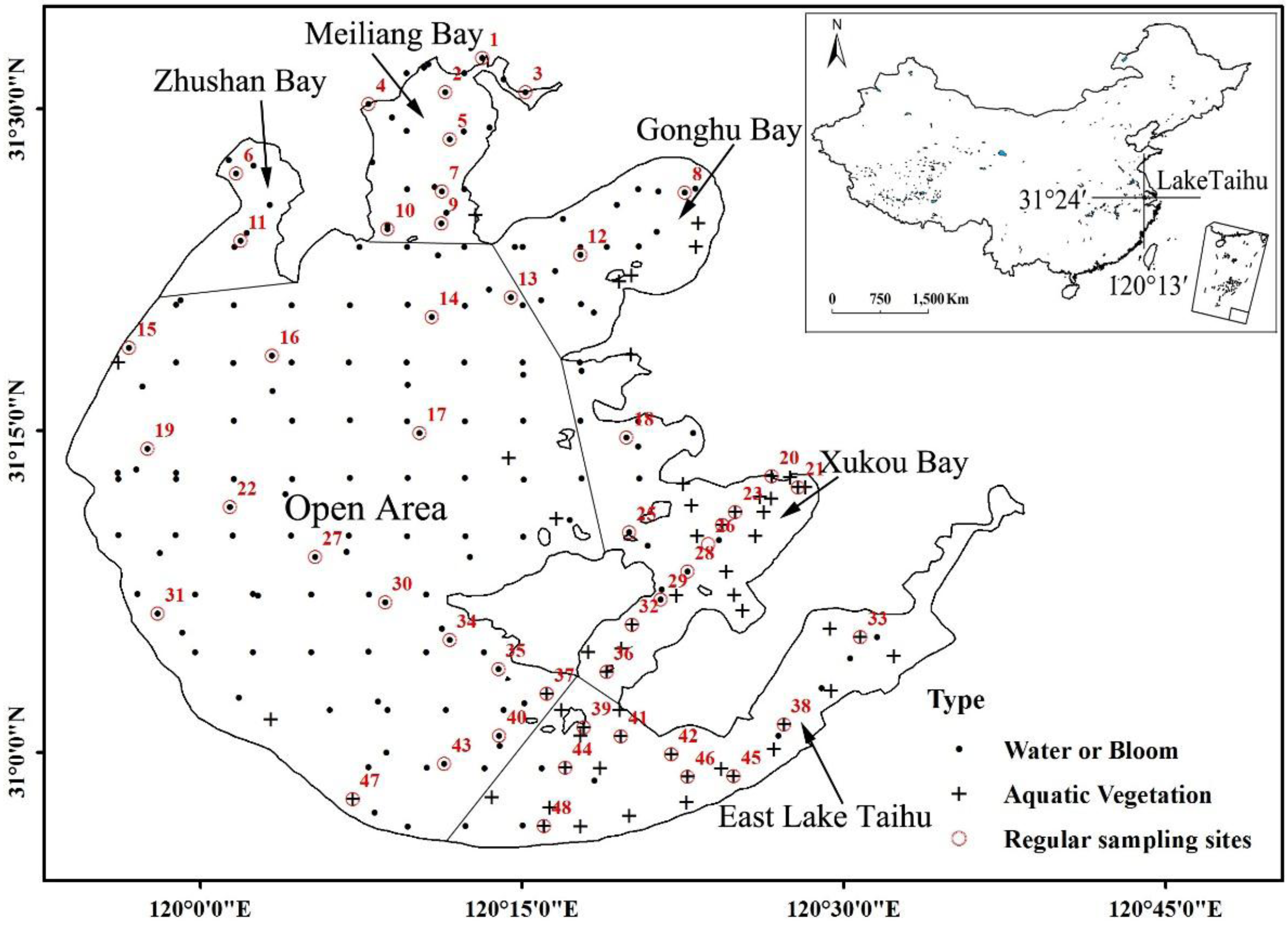
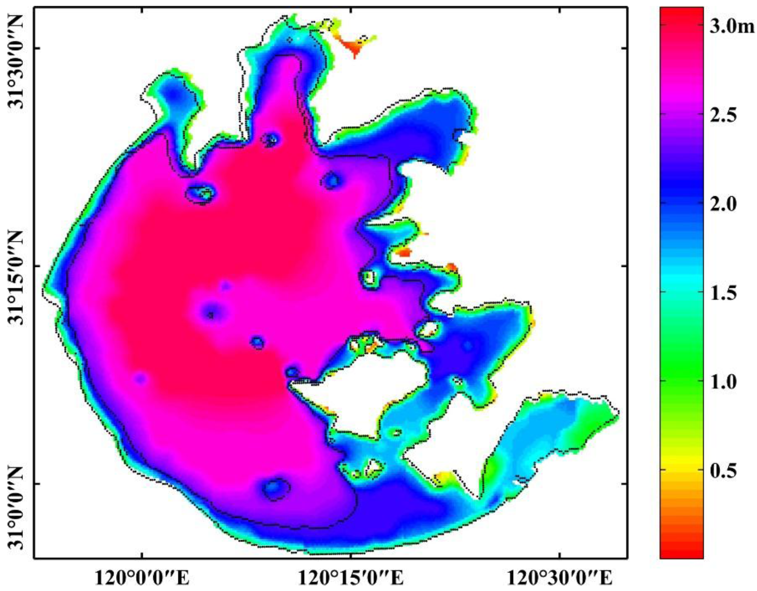
2.1. Study Area

Lake Taihu is the third largest freshwater lake in China, located between 30°55′40″–31°32′58″N and 119°52′32″–120°36′10″E. It measures 2338 km2 and has a maximum depth of less than 3.0 m and an average depth of 1.90 m [34]. Lake Taihu serves as a key drinking water resource for approximately 10 million local residents, with additional economic functions including tourism, fisheries and shipping [34].
In this typical large, shallow lake, both macrophyte-dominated and phytoplankton-dominated areas exist simultaneously. In recent decades, the excessive input of nutrients has caused severe eutrophication and algal blooms (Microcystis spp.). The algal bloom has gradually extended its coverage during this period and persists for longer durations [35]. Previous study showed the Microcystis biovolume was low in winter and early spring, and increased in late spring to a maximum in late summer and early autumn; the algae bloom began in May or June, and lasted till October [35]. In addition, the distribution of aquatic vegetation in Lake Taihu has undergone dramatic changes [36]. Human activities such as planting, harvesting and pen-fish farming have directly affected the distribution of the aquatic vegetation, causing it to fluctuate more widely [34]. Developing efficient, large-scale monitoring strategies is key to efficiently track and mitigate harmful changes in large waters bodies [3]. Therefore, there is an urgent need for an accurate estimate of the distribution of aquatic vegetation in our study area.
Generally, Lake Taihu can be divided into six areas based on the shoreline geometry, environmental factors, and human activities: Zhushan Bay, Meiliang Bay, Gonghu Bay, Xukou Bay, East Lake Taihu and the open area [14] (Figure 1). The average water depth in the six areas increases in the following order: East Lake Taihu (1.76 ± 0.37 m; average ± standard deviation), Xukou Bay (1.82 ± 0.50 m), Zhushan Bay (1.97 ± 0.54 m), Gonghu Bay (1.98 ± 0.44 m), Meiliang Bay (2.11 ± 0.63 m) and the open area (2.63 ± 0.38 m) (Figure 1 and Figure 2). The water quality is better in the southeastern part of the lake [37], and there is abundant aquatic vegetation in Xukou Bay and East Lake Taihu. The dominant species of aquatic vegetation in Lake Taihu are listed in Table 1 and are widely distributed in many other shallow lakes in China [38]. In the other areas of Lake Taihu, such as Zhushan Bay and Meiliang Bay in the north, algal blooms caused by eutrophication occur frequently [39].
Table 1. Dominant species of aquatic vegetation in Lake Taihu
TypeDominant Species
Emergent vegetationZizania caduciflora, Phragmites australis
Floating-leaved vegetationNymphoides peltatum, Trapa incisa var. sieb., Furctus Trapae Quadricaudatae
Submerged vegetationPotamogeton maackianus, Potamogeton malaianus, Vallisneria natans, Ceratophyllum demersum, Hydrilla verticillata var. roxburghii, Elodea nuttallii, Myriophyllum verticillatum, Najas minor

2.2. Field Data

A total of 482 field sites were used in this study, including a model development dataset of 244 samples and a model validation dataset of 238 samples. (1) Model development and threshold determination: Field aquatic vegetation investigations were performed along preset transects on 5–10 and 20–23 August, 1–9 September and 25 October 2013 (Figure 1, represented by black crosses and dots). A total of 244 samples were collected along these transects, and the resulting dataset was used to develop a model and determine thresholds; (2) Model validation: Forty-eight locations were sampled annually following the routine investigation launched by the Taihu Laboratory for Lake Ecosystem Research between August and October from 2008–2012 (Figure 1, represented by numbered red circles); site 45 was not sampled in 2008 and 2009. Therefore, a total of 238 samples were used to validate the method. Before the field investigation, the sampling locations were preset based on prior knowledge of the aquatic vegetation distribution and distributed approximately uniformly across the entire area.
The species and percentage coverage of the aquatic vegetation at each site were determined by eye from the boat. We placed a 5 × 5 m quadrat (parallel to the shoreline) at each station, and the main species of aquatic vegetation and their coverage within the frame were estimated and recorded (e.g., 75% species A, 25% species B).
Figure 1. The locations of 244 ground-truth samples collected in 2013 (presence of aquatic vegetation is denoted by black crosses and absence is denoted by black dots) and the annual sampling sites from 2008–2012 (represented by numbered red circles; site 45 was not sampled in 2008 and 2009); the chart in upper right box is the map of South China Sea.
Remotesensing 07 10295 g001
Figure 2. The 2003–2013 average depth distribution in Lake Taihu; the depth of 2.2 m is indicated by the black line.
Remotesensing 07 10295 g002

2.3. Image Data Description and Processing

The MODIS Aqua data were obtained beginning in 2002. MODIS Level-0 data with a 250-m resolution spanning the period 2002–2013 were downloaded from NASA and calibrated to the radiance data (Level-1b data) using SeaDAS 6.0 software. More than 4000 images covered the study area from January 2003 to December 2013. Among these, 1041 images of high quality were selected after visual examination to exclude those substantially affected by clouds, sun glare, or thick aerosols (Table 2). The gaseous absorption and Rayleigh scattering were corrected using software developed by the MODIS data processing team. The lake shore was generated using MODIS FAI data, which is described in detail by Hu et al. [24].

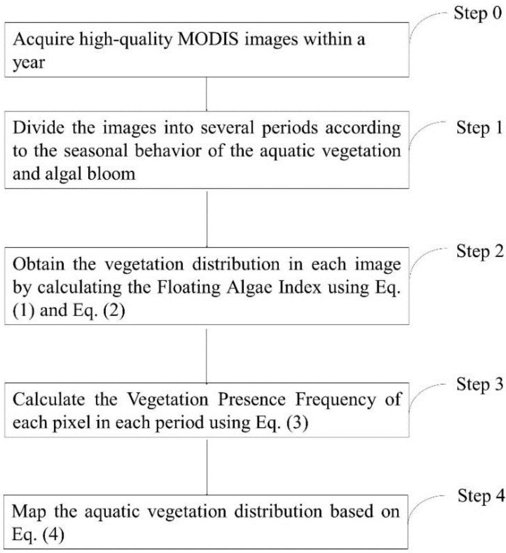
2.4. Method Description: Frequency-Based Aquatic Vegetation Mapping

Due to the difficulty of directly distinguishing algal blooms from aquatic vegetation in eutrophic aquatic ecosystems using moderate-resolution images, we used a frequency approach to delineate the areas of constant appearance of aquatic vegetation. This approach was based on the following assumption: since all of the dominate species in Lake Taihu are attached to the bottom (Table 1). Therefore, the distribution location of aquatic vegetation is relatively fixed throughout the majority of the year, whereas algae float on the water surface and often move. Floating algae were less often present than was aquatic vegetation. Therefore, aquatic vegetation and algae could be easily distinguished by establishing a presence frequency threshold. The general approach is described as follows (Figure 3):
Table 2. Temporal distribution of the MODIS-Aqua images used in this study.
20032004200520062007200820092010201120122013Total
January10835438386462
February3621582553343
March661091184747678
April712134971249101097
May4791091414761011101
June5878137544254
July71348712382101286
August91161010871127889
September9888105118138391
October14131211127141051211121
November101477121071251212108
December12714941561391210111
Total96113959094100959372101921041
Figure 3. Flow chart of the general approach.
Remotesensing 07 10295 g003
Step 0: Acquire the MODIS images within a year
Step 1: Divide the images into several periods according to the seasonal behavior of the aquatic vegetation and algal bloom
In lakes undergoing extreme eutrophication, algal blooms may be constant in certain areas, making them difficult to distinguish from aquatic vegetation using this frequency test. To prevent misclassification of areas always covered by algal blooms, we divided the year into several periods based on the growth of algae and aquatic vegetation, among which three periods were considered.
Period 1, the Wintering Aquatic Vegetation period (WAV period), spans December and January. Because of the low temperature, algae blooms are rarely observed during this period [35]. Perennial herbaceous Phragmites australis is the main species of aquatic vegetation present through the winter.
Period 2, the prolonged coexisting Algal Bloom and Wintering Aquatic Vegetation period (ABWAV period), was defined based on previous observations. Microcystis (the dominant algae species in Lake Taihu) starts to grow when the five-day average temperature is above 9 °C [40]. Deng et al. [35] evaluated the relationship between temperature and the growth of Microcystis in Lake Taihu and found that the average water temperature from 1991–2010 in March was 11 °C, making it a crucial period for the growth of Microcystis. Therefore, the five-day average water temperature in Lake Taihu reached the mentioned threshold during this period, causing the overwintering Microcystis on the surface of the sediment to grow, gain buoyancy and then float in the water column [35].
Period 3, the peak of coexisting Algal Bloom and Aquatic Vegetation period (ABAV period), spans from June to October, when the area, biomass and diversity of aquatic vegetation and the frequency of the algae bloom are both at their peak [35,41].
April, May and November were not included in the three defined periods because of the rapid variation in aquatic vegetation during these three months in Lake Taihu. Generally, the area of aquatic vegetation expands rapidly in April and May; in November, the area of aquatic vegetation rapidly decreases [42].
Step 2: Obtain the vegetation distribution in each image by calculating the Floating Algae Index
To discriminate vegetation signal from open water in the study area, we used the FAI as an indicator of both aquatic vegetation and floating algae. The FAI method has been found to be robust under virtually all conditions in the study area, including conditions affected by chromophoric dissolved organic matter, thick aerosols and frequent sun glare during the summer [24].
The FAI was calculated based on the Rayleigh-corrected reflectance (Rrc(λ), in which λ is the wavelength, nm) derived from MODIS images using the following equations [23]:
F A I = R r c ( 859 ) R r c ( 859 )
R r c ( 859 ) = R r c ( 645 ) + [ R r c ( 1240 ) R r c ( 645 ) ] ( 859 645 ) / ( 1240 645 )
Then, the area with aquatic vegetation or algae can be separated from the open water by a critical threshold, the FAI threshold (TFAI, determined in Section 3.1.1). Pixels with values greater than the TFAI were defined as vegetation signals (aquatic vegetation or algae).
Step 3: Calculate the Vegetation Presence Frequency (VPF)
This step was designed to separate the temporary floating algal bloom from the aquatic vegetation.
In our study, when the FAI of pixel j exceeded the FAI threshold (TFAI), the value of this pixel was set to 1 in the FAI layer; otherwise, the value of the pixel was set to 0. The vegetation (both aquatic vegetation and algae) presence frequency in each pixel was then evaluated in a given set of n images (per defined period):
V P F ( j ) = i = 1 n F A I ( j , i ) n
where VPF is the vegetation presence frequency of the pixel j in the image set of n and represents the proportion of pixel j with FAI = 1 in the total number of images (n). Thus, a pixel j that was assigned a value of 1 in every FAI layer of the set n would be assigned a value of 1 in the VPF layer; a pixel j that was assigned a value of 0 in every FAI layer of the set n would be assigned a value of 0 in the VPF layer.
Thereafter, the temporary floating algae could be separated by setting a VPF threshold; when this critical threshold was exceeded in a defined period, this pixel was classified as a vegetation signal. The VPF thresholds of the three periods were defined separately.
Step 4: Map the aquatic vegetation distribution based on FAI and VPF
This step was designed to prevent the prolonged floating algae from being classified as aquatic vegetation by seasonal phenology comparison and water depth limitation.
In this step, we first defined the critical VPF of each period to exclude the area covered by temporary floating algae, and therefore quantify the distribution of vegetation signal in each period. After comparing the VPF acquired area among three defined periods, the influence of long-term algal bloom can be eliminated.
Secondly, we used the maximum depth of aquatic vegetation colonization to further regulate the classification in our approach. A previous study in Lake Taihu found that the aquatic vegetation occurs at a water depth less than 2 m [14]. In our study, a water depth of < 2.2 m was used to improve the classification accuracy of aquatic vegetation considering findings from other similar published studies [43].
Hence, the distribution of the aquatic vegetation can be classified using the following equation:
A a v = A ( T 3 ) A ( T 2 ) + A ( T 1 ) A ( d e p t h )
where Aav is the area of aquatic vegetation; T1, T2 and T3 are the VPF thresholds of the defined periods 1, 2 and 3, respectively; A(T1), A(T2) and A(T3) are the areas where the VPF thresholds of T1, T2 and T3 are exceeded, respectively; and A(depth) is the area of water depth greater than 2.2 m. The 2003–2013 averaged water depth distribution is shown in Figure 2.
The VPF thresholds of T1, T2 and T3 were determined based on the analysis of satellite-generated maps and the 244 in situ samples collected in 2013. The robustness of the frequency method and the determined thresholds were then assessed using the validation datasets from 2008–2012.

2.5. Classification Accuracy Assessment

The agreement between the estimated aquatic vegetation areas and ground-truth measurements was assessed based on the user’s accuracy and the overall accuracy. The user’s accuracy (pu(i)) is a measure of the commission error associated with a class and is derived from the number of pixels correctly allocated to a class relative to the total number of pixels predicted to belong to that class in the accuracy assessment [44]:
p u ( i ) = p c ( i ) p t ( i )
where pc(i) is the number of correctly classified pixels of type i, and pt(i) is the number of total pixels of type i based on the ground-truth measurements.
The overall accuracy (po) was defined as the percentage of samples that were classified correctly and calculated using the following equation:
p o = i = 1 n p c ( i ) p t
where n is the total number of types that were classified, pc(i) is the number of correctly classified pixels of type i, and pt is the total number of pixels in the validation data set.
To verify the stability and accuracy of the model, the user’s accuracy and the overall accuracy were calculated by comparing the satellite-derived aquatic vegetation distribution to the ground-truth results during 2008 and 2012.

2.6. Statistical Analyses

Statistical analyses, including average value and non-liner fitting, were performed with SPSS 18.0 software (Statistical Program for Social Sciences). The correlations were evaluated using p-values and were considered significant at p < 0.05.

3. Results

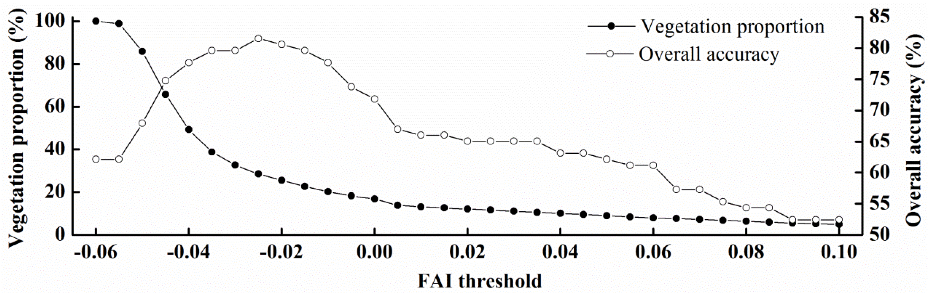
3.1. Threshold Determinations

3.1.1. FAI Threshold Determination for the Detection of Aquatic Vegetation in Lake Taihu

The FAI threshold of −0.004 was initially developed by Hu et al. [24] to distinguish bloom and non-bloom waters. This threshold was based on FAI gradients and statistics without the validation of ground-truth. Therefore, this threshold may introduce potential uncertainty when directly applying it to the classification of aquatic vegetation.
To determine the appropriate TFAI for the detection of aquatic vegetation in Lake Taihu, an image from 8 August 2013 was selected to evaluate the overall accuracy of various FAI thresholds. A total of 104 in situ observations were used for the determination of TFAI. The ground-truth of open water and thick algal bloom were defined according to an observation during 5–10 August 2013. The weather was clear and calm during this transect, with an average wind speed of 3.10 m/s. Because the position of the aquatic vegetation remains stable during June and October in Lake Taihu, all of the sites of aquatic vegetation collected in 2013 were used in this test.
With the increase of the TFAI, the defined proportion of the lake containing aquatic vegetation decreased. We increased the TFAI in 0.005-step increments and evaluated the overall accuracy of the satellite-derived vegetation signal distribution based on the ground-truth data. With an increase in TFAI from −0.06 to 0.10, the overall accuracy increased from 62%–82% and then decreased to 52%; the highest accuracy was obtained when the TFAI as −0.025 (Figure 4). To further analyze the variation in classification accuracy with changes in the TFAI, vegetation signal distribution maps were generated based on TFAI values of −0.04, −0.025 and −0.004 (Figure 5). The best agreement between the derived results and the ground-truth data indicated an overall accuracy of 82% (Figure 4 and Figure 5) when the TFAI was −0.025. When the TFAI was −0.04, 50% of the lake was classified as covered with vegetation signal, and the overall accuracy was 78%. The greatest levels of disagreement between the derived and actual vegetation signal distributions were observed in Meiliang Bay and Gonghu Bay. When a TFAI of −0.004 was used as the threshold of floating algal detection [24], 14% of the lake was classified as covered with vegetation signal, and the overall accuracy was 70%. The aquatic vegetation area was significantly underestimated in Xukou Bay. Therefore, a more accurate TFAI of −0.025 was used in our subsequent analysis. The threshold we used is lower than that determined by Hu et al. 2010 [24]. Hu et al. used the FAI threshold of −0.004 to separate the bloom and nonbloom waters in Lake Taihu, and no concurrent filed investigation result was used for the validation of their threshold [24]. Therefore, there could be some uncertainties for that critical threshold. Differently, in our study, the threshold was determined and validated with the concurrent field data. Regarding this, we strongly recommend to use the value of −0.025 as the classification threshold in Lake Taihu.
Figure 4. Variation in vegetation signal coverage proportion and overall accuracy with variation in the FAI threshold on 8 October 2013.
Remotesensing 07 10295 g004
Figure 5. Variation in the area classified as vegetation signal on 8 October 2013 with FAI thresholds of (a) −0.04, (b) −0.025 and (c) −0.004. Aquatic vegetation at the locations is denoted by black crosses, and thick floating algal blooms are denoted by red crosses. The black dots denote locations of open water.
Remotesensing 07 10295 g005

3.1.2. Separating the Aquatic Vegetation and Floating Algae Based on VPF

The aquatic vegetation covered the largest constant area in Lake Taihu during the phenologically defined “Coexisting Algal Bloom and Aquatic Vegetation period” (June to October). Accordingly, the VPF threshold of the ABAV period (T3) was defined as 0.85 to distinguish the temporary floating algal area based on the ground-truth data, meaning that an area was classified as having a vegetation signal when a vegetation signal was detected more than 85% of the time.
These areas covered by prolonged algal blooms could not be removed by setting the VPF threshold in the ABAV period (T3). The VPF threshold of the WAV period (T1) and ABWAV period (T2) were then determined with T3 set to 0.85. We used the T1 to estimate the wintering aquatic vegetation area in the WAV period and the T2 to estimate the prolonged algal bloom and wintering aquatic vegetation area in the ABWAV period. Based on the phenological vegetation frequency analysis from 2003 to 2013 (Figure 6) and the field investigation in 2013, Zhushan Bay and Meiliang Bay were frequently covered by Phragmites australis along part of the lakeshore. The percentages of aquatic vegetation coverage in Zhushan Bay and Meiliang Bay in 2013 were less than 20% and 10%, respectively. The percentage of aquatic vegetation coverage in East Lake Taihu was approximately 70% in 2013. We evaluated the defined aquatic vegetation percentage in Zhushan Bay, Meiliang Bay and East Lake Taihu using thresholds of T1 and T2 ranging from 0.35 to 0.95. The aquatic vegetation percentage in the three areas agreed with the ground-truth measurements when T1 and T2 were between 0.45 and 0.65. The overall accuracy was highest, i.e., 84%, when T1 and T2 ranged from 0.50–0.65 and from 0.45–0.55, respectively. The T2 threshold range of 0.45–0.55 performed best in identifying those areas with prolonged algal blooms or wintering aquatic vegetation in February and March. To better capture the area with prolonged algal blooms, the threshold of T2 was set to 0.45. The T1 threshold range of 0.5–0.65 performed best in mapping the wintering aquatic vegetation in December and January in Lake Taihu. Some of the best results were obtained when we set T1, T2 and T3 to values of 0.55, 0.45 and 0.85, respectively. These thresholds were then used in the mapping of aquatic vegetation from 2003–2012.

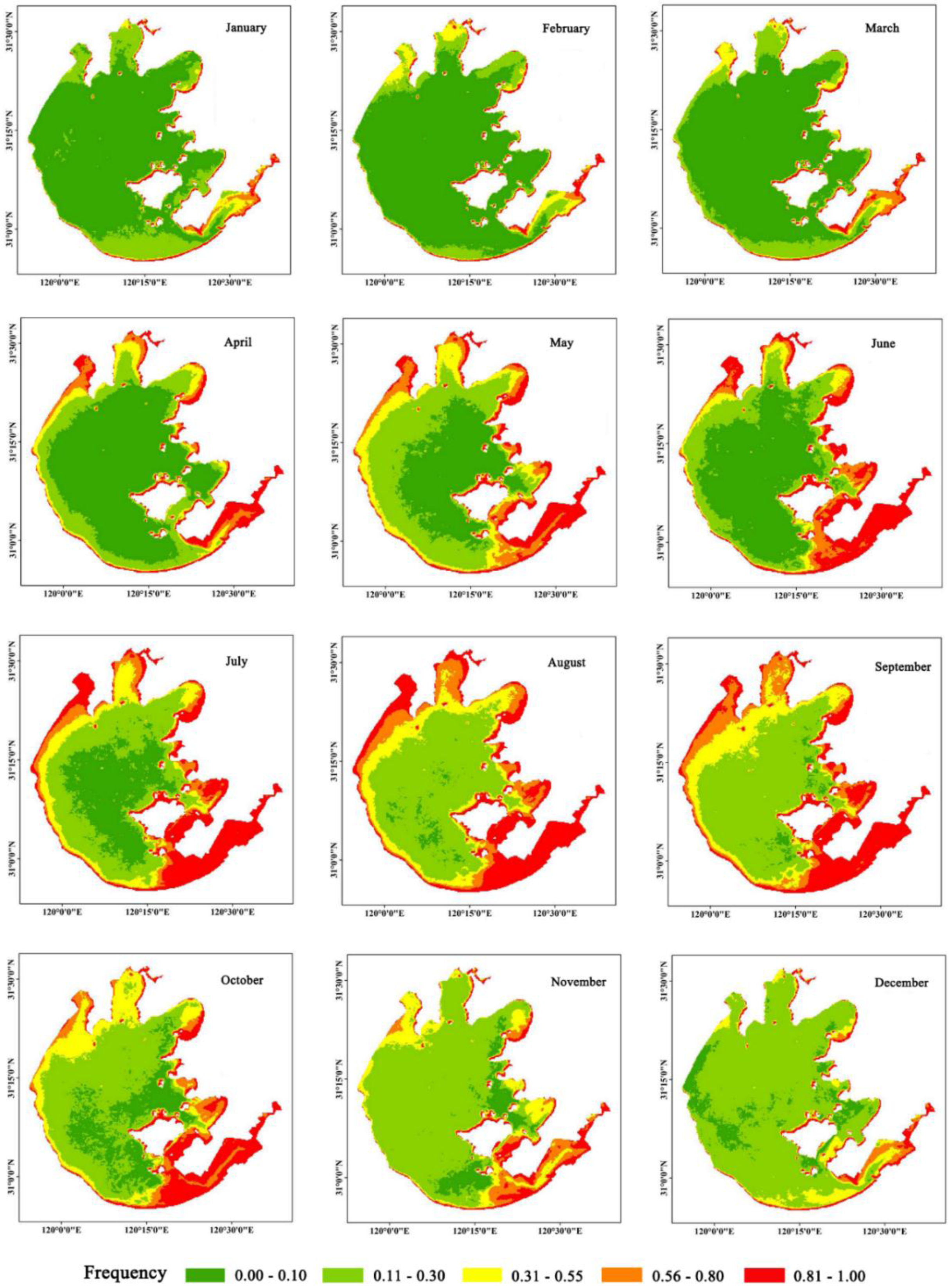
3.2. Phenological Variation in Vegetation Signal Distribution

The monthly variation in the frequency of the appearance of vegetation signals is shown in Figure 6. The distribution pattern was similar in December and January; i.e., the vegetation signal appeared frequently in the littoral zone and East Lake Taihu but was rare elsewhere. Based on our investigation, the majority of aquatic vegetation in December and January consisted of Phragmites australis. Phragmites australis is a perennial herbaceous aquatic plant that is primarily present in the southern and western littoral zone and in East Lake Taihu [29]. In February and March, the high-frequency vegetation areas expanded, particularly in Xukou Bay and Meiliang Bay. The expansion of vegetation signal during this period can be partly attributed to the growth of the overwintering Microcystis in the sediment [35]. In April and May, due to the growth of the aquatic vegetation and algae, the high-frequency vegetation areas increased dramatically in Zhushan Bay, Meiliang Bay, Xukou Bay and East Lake Taihu. From June to October, the high-frequency vegetation areas remained approximately constant, and the largest high-frequency vegetation area was in Lake Taihu [41,45]. From October to November, the areas with a vegetation signal decreased significantly, particularly in Meiliang Bay and Xukou Bay (Figure 6). From November to October, the vegetation areas in Zhushan Bay, Gonghu Bay, Xukou Bay and East Lake Taihu continued to decrease (Figure 6).
Combining the vegetation presence frequency threshold we defined for T1 and T2 and the monthly vegetation frequency presented in Figure 6, the regional ecological type of Lake Taihu during the WAV period and ABWAV period was obtained. In December and January (T1 = 0.55), the wintering aquatic vegetation was primarily distributed in the bay of East Lake Taihu and along the southern and eastern lake shores (Figure 6). In February and March (T2 = 0.45), algae began to float on the water in areas of high eutrophication, such as Zhushan Bay and Meiliang Bay (Figure 6).
Figure 6. MODIS-Aqua-derived (2003–2013) monthly climatology Floating Algae Index frequencies.
Remotesensing 07 10295 g006

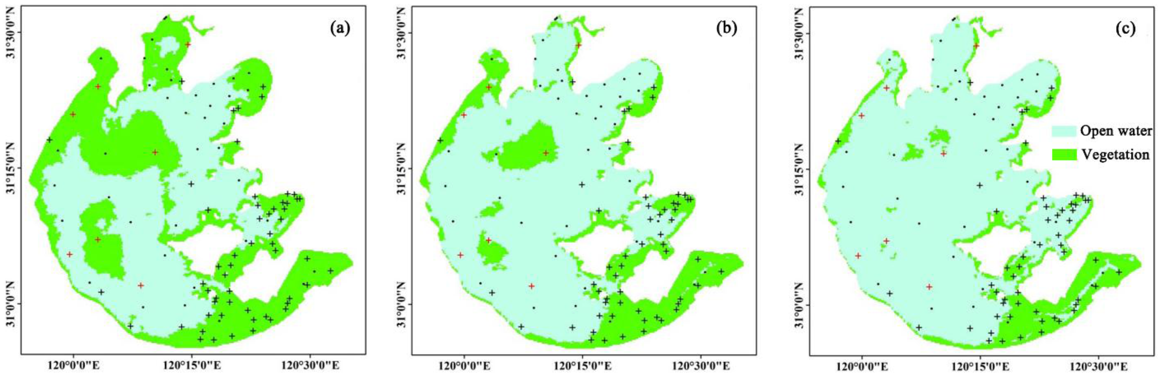
3.3. Validation of the Method Based on Field Investigation

To verify the stability and accuracy of the model, we applied the model to images from 2008–2012 and mapped the aquatic vegetation distribution accordingly (Figure 7). From 2008–2012, the user’s accuracy of the aquatic vegetation each year was 91%, 80%, 67%, 86% and 68%, respectively, and the overall classification accuracy was 87%, 81%, 77%, 88% and 73%, respectively (Table 3). The number of sites with aquatic vegetation decreased from 22 sites in 2008 to 20 sites in 2009 and 12 sites in 2010; it then increased to 19 sites in 2012. Similarly, the satellite-generated area of aquatic vegetation distribution decreased from 503.38 km2 in 2008 to 414.50 km2 in 2009 and 290.94 km2 in 2010; it then increased to 360.38 km2 in 2012 (Figure 7). The satellite-generated maps precisely showed the decrease in aquatic vegetation coverage in East Lake Taihu from 2008–2010 and the increases in 2011 and 2012, which match the results of the field investigation. The overall accuracy was relatively low when the coverage of aquatic vegetation was smaller. The sampling sites were at the same locations each year. When the coverage of the aquatic vegetation decreased, some of the stations were covered by extremely sparse aquatic vegetation, making it undetectable from MODIS images. We discuss the limitation of the spatial resolution problem in the Discussion section. The overall accuracy could be slightly overestimated or underestimated for two reasons: first, the generated overall accuracy was obtained from limited ground-truth data in each year; second, considering the distribution of the aquatic vegetation, the pre-set ground-truth data were not completely uniformly distributed, being denser in East Lake Taihu.
Several sites dominated by Potamogeton malaianus were classified as open water, such as sites 28 and 37 in 2008 and 2009 and sites 37 and 44 in 2011 and 2012 (Figure 1 and Figure 7). Potamogeton malaianus, which belongs to the Potamogetonaceae, is a common summer submerged macrophyte species in Chinese lakes. However, this mismatch was not observed in other areas dominated by submerged macrophyte species, such as site 42 in 2008 (Hydrilla verticillata var. roxburghii), site 20 in 2009 (Ceratophyllum demersum), site 21 in 2010 (Vallisneria natans), site 42 in 2011 (55% Vallisneria natans and 45% Ceratophyllum demersum) and site 19 in 2012 (75% Potamogeton maackianus, 15% Myriophyllum verticillatum, 5% Hydrilla verticillata var. roxburghii and 5% Nymphoides peltatum) (Figure 1 and Figure 7), which indicates that our approach works well on various dominant types of submerged vegetation in Lake Taihu except Potamogeton malaianus.
Table 3. Accuracy assessment of classification results from 2008–2012.
YearMeasuredPredicted
Aquatic VegetationOpen WaterUser’s AccuracyOverall Accuracy
2008Aquatic vegetation20291%87%
Open water42184%
2009Aquatic vegetation16480%81%
Open water52281%
2010Aquatic vegetation8467%77%
Open water72981%
2011Aquatic vegetation19386%88%
Open water32388%
2012Aquatic vegetation13668%73%
Open water72276%
In order to verify the accuracy of our method in different depth conditions, we further divided all the validation sites into three classes following the water depth distribution in each region (Figure 1 and Figure 3): large-depth region, including Open Area and Meiliang Bay, where 24 sites were sampled; medium-depth region, including the Gonghu Bay and Zhushan Bay, where the measurements were made at four sites; shallow-depth region, including the East Lake Taihu and Xukou Bay, where 20 sites were observed. The overall accuracy in each depth class from 2008–2012 was 84%, 94% and 76%, respectively. The general performance of our approach was stable in different type of water depth regions, with a relatively lower accuracy in the shallow region.
Figure 7. Distribution of aquatic vegetation from 2003–2013 and the distribution based on ground-truth measurements from 2008–2012. The presence of aquatic vegetation at the locations is denoted by black crosses and the absence of aquatic vegetation is denoted by black dots.
Remotesensing 07 10295 g007

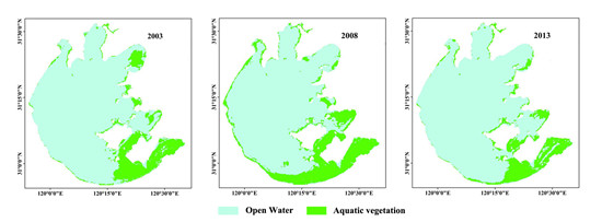
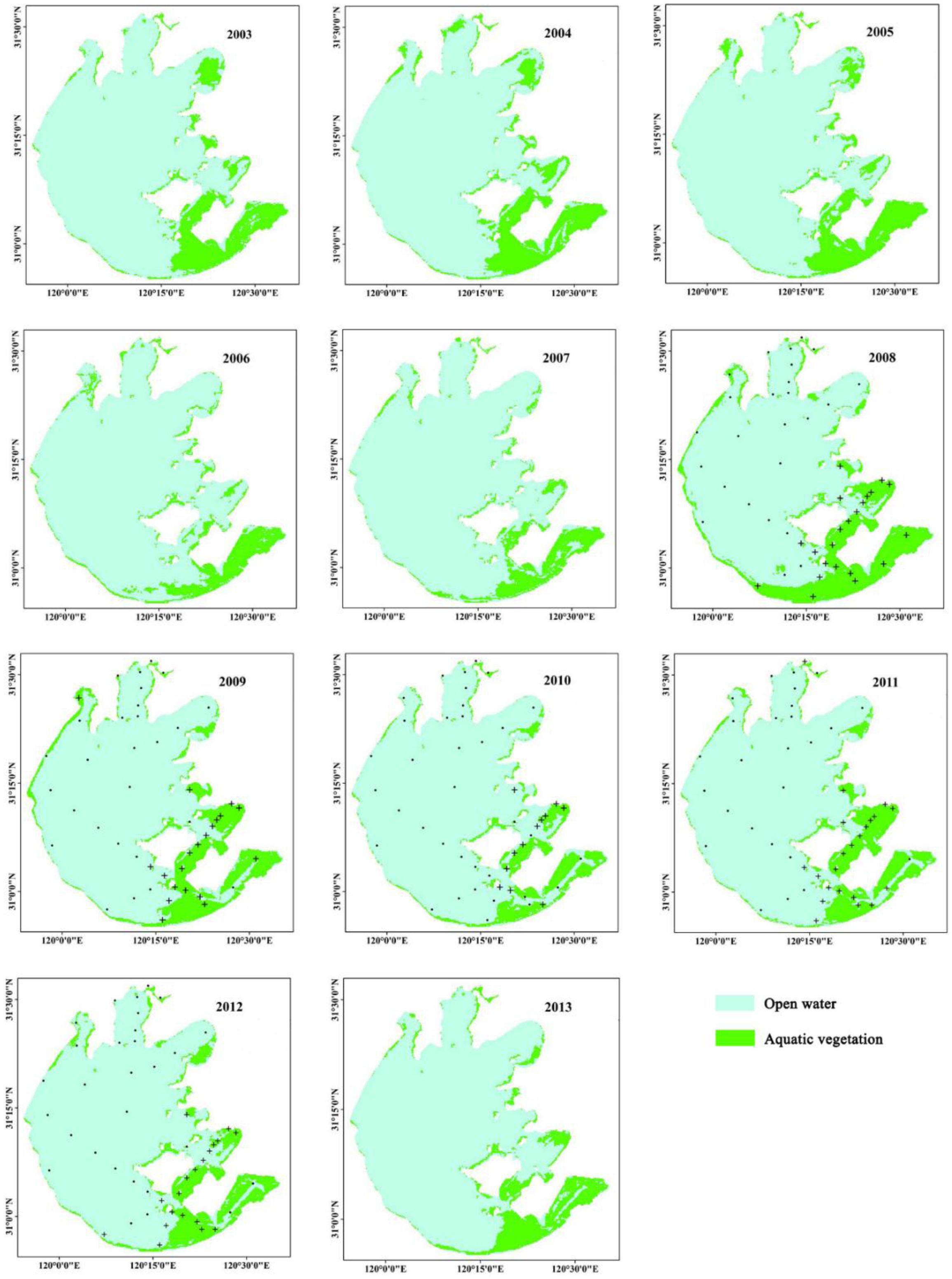
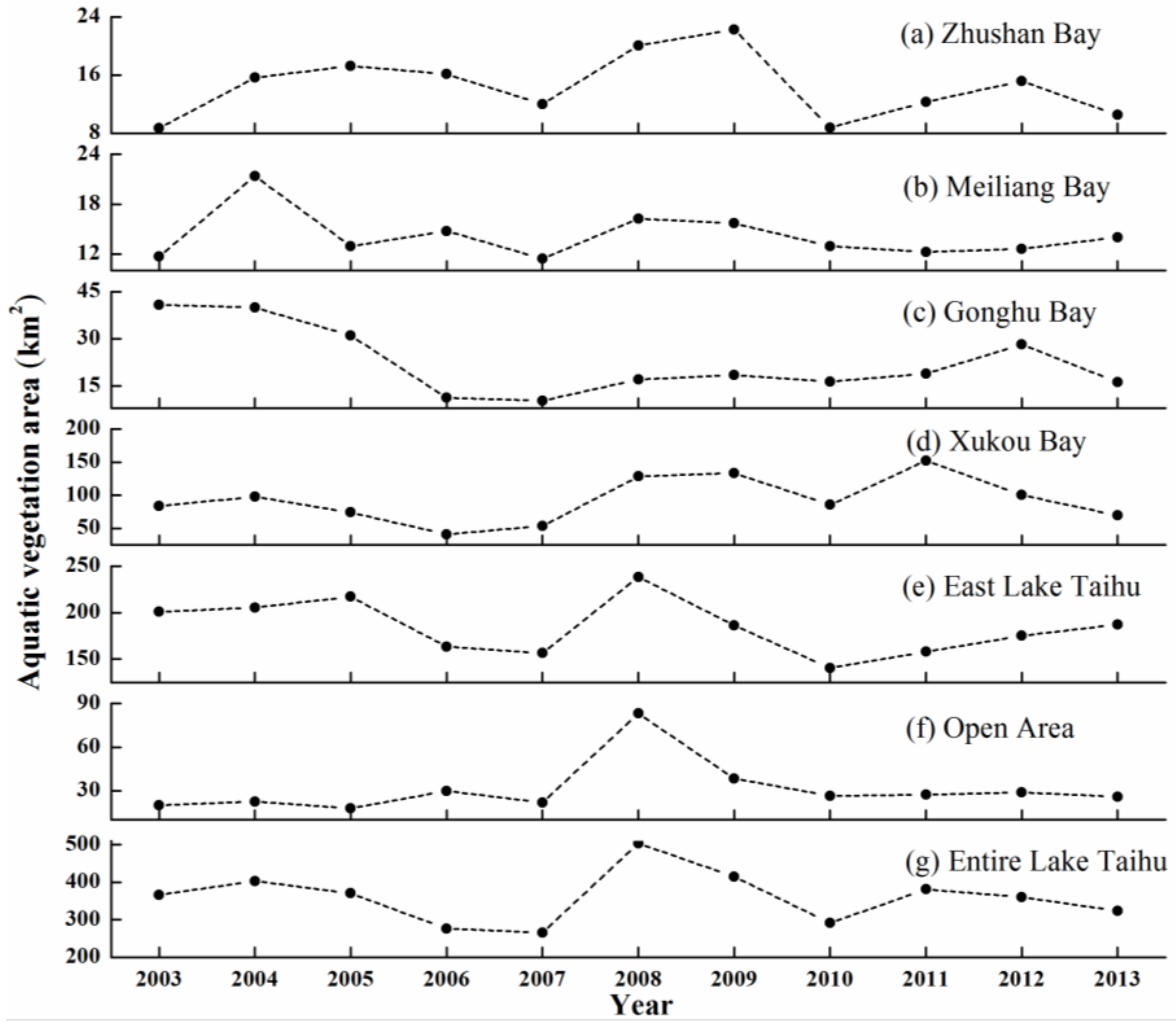
3.4. Spatial and Temporal Dynamics of Aquatic Vegetation Distribution

From 2003–2013, the aquatic vegetation was distributed primarily in the eastern part of Lake Taihu (Figure 7). During these 11 years, the spatial pattern of the distribution underwent some noticeable changes, particularly in Gonghu Bay and Xukou Bay (Figure 7 and Figure 8). The total area of aquatic vegetation ranged from the lowest value of 265.94 km2 in 2007 to the highest value of 503.38 km2 in 2008, with average coverage of 359.62 km2 over the 11 years.
Figure 8. Satellite-derived areas of aquatic vegetation area: (a) Zhushan Bay, (b) Meiliang Bay, (c) Gonghu Bay, (d) Xukou Bay, (e) East Lake Taihu, (f) Open Area and (g) Entire Lake Taihu.
Remotesensing 07 10295 g008
To further analyze the distribution of the aquatic vegetation, the temporal variation in the derived area of aquatic vegetation from 2003–2013 in the six zones (Zhushan Bay, Meiliang Bay, Gonghu Bay, Open Lake Taihu, Xukou Bay and East Lake Taihu) and over the entire lake was analyzed (Figure 8). The 11-year average coverage of aquatic vegetation in these six areas was as follows, in decreasing order: East Lake Taihu (184.40 km2, 64.6% of the area), Xukou Bay (92.86 km2, 37.4% of the area), Open Lake Taihu (31.13 km2, 2.2% of the area), Gonghu Bay (22.63 km2, 13.6% of the area), Zhushan Bay (14.43 km2, 20.5% of the area) and Meiliang Bay (14.18 km2, 11.6% of the area). East Lake Taihu and Xukou Bay accounted for 51.9% and 25.8% of the averaged total aquatic vegetation coverage from 2003–2013, respectively. In addition, the trends were similar in East Lake Taihu, Xukou Bay and over the entire Lake Taihu, which displayed relatively larger areas of aquatic vegetation in 2008, 2009 and 2011 and smaller areas of aquatic vegetation in 2006 and 2007 (t-test, p < 0.001).

4. Discussion

4.1. Advantages and Limitations of the Proposed Approach

4.1.1. Advantages of the Proposed Approach

It is difficult or impossible to accurately estimate the historical distribution of aquatic vegetation without using field observations and remote sensing images simultaneously [29]. An empirical estimation model was developed based on field observations and concurrent satellite imagery and was then used on the past satellite imagery.
Accurately distinguishing the vegetation signal from the water area is the first step in accurately estimating the distribution of aquatic vegetation using remote sensing. This step can be achieved using the vegetation index with various band combinations or classification methods. However, in inland waters and coastal areas undergoing eutrophication, algal blooms frequently coexist with aquatic vegetation [31,33], which poses another difficulty in the accurate estimation of the distribution of aquatic vegetation.
Some previous studies involving separating the signals of aquatic vegetation and algal blooms in Lake Taihu were performed by masking the “phytoplankton-dominated region” based on prior knowledge [28,29]. However, according to our investigation, the “phytoplankton-dominated regions” such as Zhushan Bay, Meiliang Bay, Gonghu Bay and the open lake were also areas of aquatic vegetation, which was verified by other studies [46]. In addition, simply removing the “phytoplankton-dominated region” when retrieving the aquatic vegetation distribution through satellite images does not allow for discernment of long-term alternations of the ecological stages. Several previous studies of Lake Taihu eliminated the influence of algae by comparing the differences among seasons [36,47]. However, both the aquatic vegetation and the algal blooms were at their largest and smallest extents within the same seasons (Figure 6); therefore, the influence of algae could not be completely removed by simple seasonal comparison.
In our study, the aquatic vegetation distribution was determined by combining the frequency test and seasonal phenology comparison. The frequency test during June and October easily separated the temporary floating algae, and the frequency-based seasonal phenology comparison excluded the influence of long-term algal blooms, thereby demonstrating its utility in mapping the aquatic vegetation in a complex water ecosystem undergoing eutrophication.
This frequency based conception on aquatic vegetation detection in eutrophic waters is a novel attempt, and has the potential to be applied in other eutrophic waters in multiple stable states.

4.1.2. Limitations of the Proposed Approach

However, there are some limitations to our presented approach. First, the spatial resolution of the MODIS data we used is 250 m, making it difficult to identify small clumps of aquatic vegetation. A comparison between a Landsat/ETM+ image with 30-m resolution and the corresponding MODIS FAI image showed that a surface slick is detectable on the MODIS FAI imagery if its width is larger than 60 m [23]. Therefore, we attempted to compensate for this limitation using Landsat data for small-sized floating algae and aquatic vegetation clusters. However, available Landsat data were very limited due to the temporal resolution of 16 days and the severe air pollution in this region in the summer [48]. On the USGS website, by setting the maximum cloud coverage at 40%, only 39 Landsat-5 images in the Lake Taihu area were eligible, with less than 30 images that could actually be used in our study. More importantly, only five valid Landsat-8 images (high quality and with low cloud coverage) in the Lake Taihu area could be used for mapping aquatic vegetation from 2013 to the present [49]. Due to the coexisting ABAV period from July to October, the effect of algae could not be removed by a comparison of only several images. We expect to collect additional high spatial resolution images to compensate for this limitation and obtain more accurate estimates of the spatial distribution of aquatic vegetation in the future.
Regarding the limitation of the MODIS image resolution, the accuracy of our proposed approach would be related to the coverage area of the sampling sites. When the coverage of the aquatic vegetation decreased, some of the stations were covered by extremely sparse aquatic vegetation, making it undetectable from MODIS images. In this context, the yearly variation of user’s accuracy and overall accuracy can be explained: both the user’s accuracy and the overall accuracy were relatively low when the coverage of aquatic vegetation was smaller. The aquatic vegetation coverage was smaller in 2010 (290.94 km2) and 2012 (360.38 km2), and was larger in 2011 (380.81 km2), 2009 (414.50 km2) and 2008 (503.38 km2). Correspondingly, the user’s accuracy of aquatic vegetation increased from 67%–91%. Similarly, the overall accuracy was relatively low in 2010 (77%) and 2012 (73%), and much higher in 2011 (88%), 2009 (81%) and 2008 (87%).
Second, one species of submerged aquatic vegetation was difficult to detect in our study: Potamogeton malaianus. Water strongly absorbs electromagnetic radiation in the optical region, resulting in significant damping of the radiometric signal and thereby posing difficulties in satellite remote sensing of submerged aquatic vegetation [50]. Future attempts to accurately address Potamogeton malaianus should be used to develop more accurate estimates of the aquatic vegetation distribution in Lake Taihu.
Third, there are also limitations regarding the validation data set used in this study. First, the sampling sites were not completely uniformly distributed, as denser sampling sites were distributed in the eastern Lake Taihu. Second, only 48 sites were included in each validation dataset. These two limitations may lead to overestimation or underestimation of the retrieving accuracy. However, the dense sampling sites distributed in the macrophyte-dominated area are expected to more accurately capture the change in the distribution of aquatic vegetation and therefore facilitate the evaluation of the efficiency of our proposed method in monitoring the variation in aquatic vegetation coverage.
In addition, we emphasize that our proposed approach may need further adjustment when applied to other eutrophic waters, considering the following facts. Firstly, the division of the different period is related to the phonological character of the study area. Secondly, the maximum depth of aquatic vegetation colonization may vary in different types of waters, mainly influenced by the water transparency. Thirdly, the threshold of the VPF may have slight variation in different waters, relating to the appearance frequency of algal bloom. Calibration and validation are still needed in other eutrophic waters before the proposed novel approach is applied to other localities. It should also be noted that this appearance frequency based approach may fail in the area dominated by quite mobile aquatic vegetation such as water hyacinth.

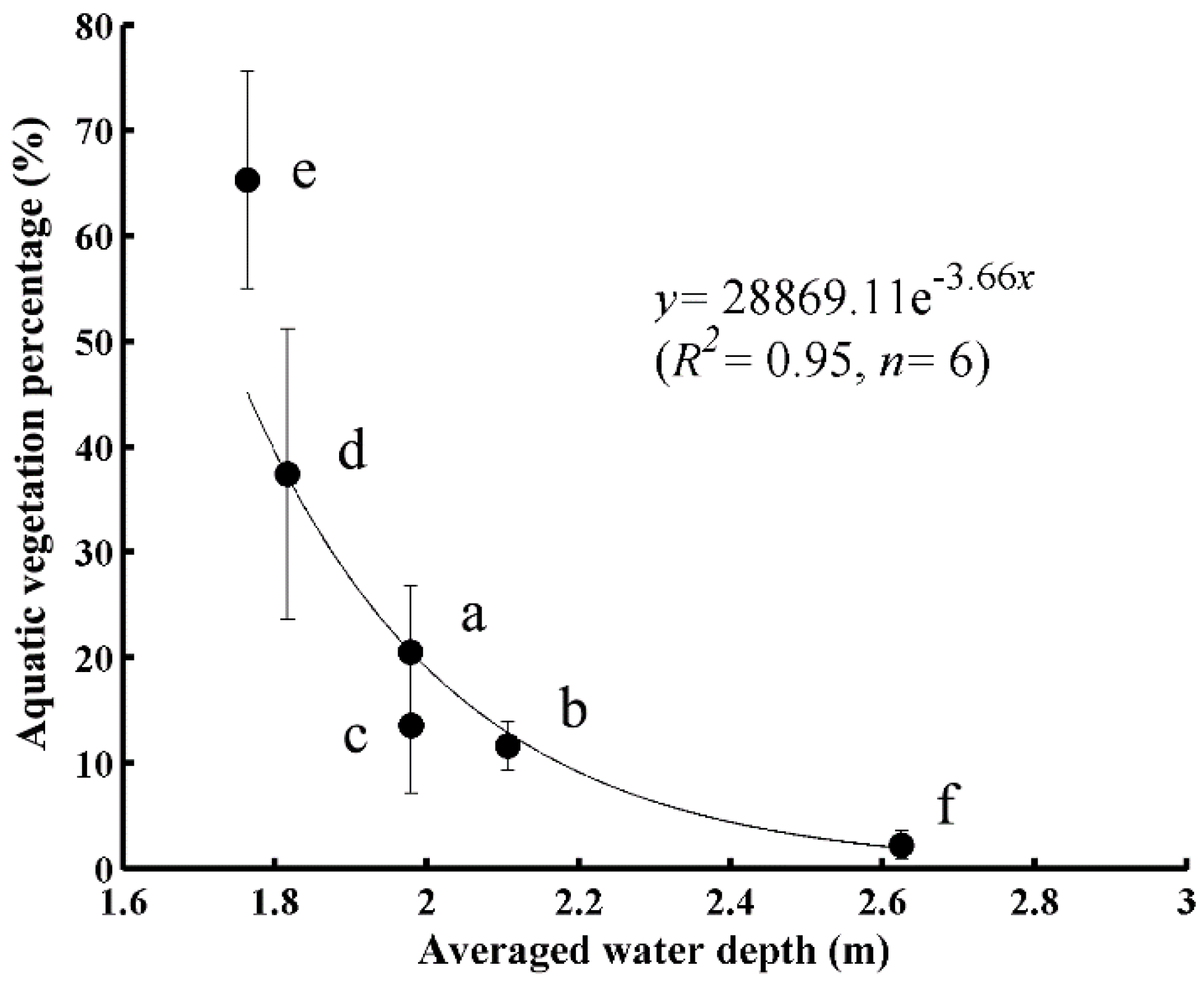
4.2. Factors Affecting the Spatial and Temporal Variation of Aquatic Vegetation

4.2.1. Direct and Indirect Effects of Human Activities

Human activities have greatly affected the spatial and temporal variation of aquatic vegetation in Lake Taihu during the past few decades. Pen-fishing is the main form of aquaculture in Lake Taihu [34]. The area of pen-fish farming area exceeded 60 km2 from 2003–2007 and then decreased to less than 40 km2 from 2008–2010 [36]; correspondingly, the average aquatic vegetation area increased from 336.45 ± 61.35 km2 (average from 2003–2007) to 402.94 ± 106.69 km2 (average from 2008–2010).
The indirect effects of human activities on the aquatic vegetation are more complex than the direct effects from activities such as planting or harvesting. The decrease of aquatic vegetation in Gonghu Bay in recent years can be explained by a series of effects from high nutrient water input: The average volume of water entering Gonghu Bay from the Yangtze River via the Wangyuhe River was approximately 0.8 billion m3 per year from 2003–2008 [51]. The input of flushing water from the Yangtze River through Gonghu Bay often contains higher nutrient concentrations than the lake itself [51]. The total phosphorus concentration in the water from the Yangtze River (~0.1 mg/L; [52]) is greater than that in the majority of the lake (~0.03–0.09 mg/L; [51]), except in Meiliang Bay and Zhushan Bay. More importantly, the concentration of total suspended matter in the lower Yangtze River is higher than that of Gonghu Bay [14,53]. The underwater light supply is a key factor determining the growth and distribution of aquatic vegetation; the increased nutrient loading is expected to increase the nutrient level in Gonghu Bay and promote the growth of algae, and the increased loading of total suspended matter is expected to increase the turbidity and thereby reduce the underwater light supply and decrease the area of aquatic vegetation [30]. In Gonghu Bay, the average area of aquatic vegetation was 37.31 ± 5.37 km2 from 2003–2005 and sharply decreased to 17.12 ± 5.47 km2 during the period from 2006 to 2013. Eutrophication causing serious algal blooms is another factor that decreased the area of aquatic vegetation. A serious algal bloom occurred in May 2007 and caused a severe drinking-water crisis [39]. A massive bloom is expected to greatly influence the underwater light environment and prevent the growth of aquatic vegetation; as a result, the area of aquatic vegetation in 2007 was the smallest observed in the 11-year study, with a value of 265.94 km2 (Figure 7 and Figure 8).

4.2.2. Lake Topography and Wind Wave Disturbance

The lake topography affects the water depth of the lake, which is considered responsible for variation in the biomass and species composition of aquatic vegetation in many freshwater ecosystems of the world [54,55,56]. The optimum depth for the growth of the aquatic vegetation in Lake Taihu has been reported as less than 2.0 m [14,41]. Similar findings were obtained in other studies of coastal and shallow lakes [43,57]. The average water depth in the six areas of the present study increased in the following order: East Lake Taihu (1.76 ± 0.37 m; average ± standard deviation), Xukou Bay (1.82 ± 0.50 m), Zhushan Bay (1.97 ± 0.54 m), Gonghu Bay (1.98 ± 0.44 m), Meiliang Bay (2.11 ± 0.63 m) and the open area (2.63 ± 0.38 m). Correspondingly, the proportion covered by aquatic vegetation decreased in the same order following an exponential function with a determination coefficient of 0.95 (n = 6) (Figure 9). The annual water level of Lake Taihu varied from 3.05 m–3.38 m, with an average of 3.18 m from 2000–2010 [58]. The intra-annual variation in the water level of Lake Taihu has been very low for last decades, with an average annual coefficient of variation of less than 5.00%. The average monthly coefficient of variation was 5.41% from 2000–2010 [58]. Therefore, the annual water level variation during our study period had a relatively small effect on the distribution of aquatic vegetation [58].
Figure 9. Relationship between average water depth and the percentage covered by aquatic vegetation in the six regions: (a) Zhushan Bay, (b) Meiliang Bay, (c) Gonghu Bay, (d) Xukou Bay, (e) East Lake Taihu and (f) Open Area.
Remotesensing 07 10295 g009
Large, shallow lakes are highly dynamic environments. Of all of the dynamic disturbance effects, wind-induced sediment resuspension most directly reduces water transparency and the euphotic depth and thereby influences the spatial and temporal distribution of aquatic vegetation directly and indirectly [9]. The lake topography controls the impact exerted by the wind fetch [14,59,60]. Consequently, the aquatic vegetation is primarily distributed in bays or along the lakeshore, where there is less exposure to disturbance by wind.

4.2.3. Implications for Aquatic Vegetation Restoration in Lake Taihu

In Lake Taihu, the nutrient concentrations are high, such that the growth of aquatic vegetation is controlled primarily by light availability [9,61,62]. The monthly frequency test in our study indicates that the crucial period for the growth of aquatic vegetation is from March to May in Lake Taihu (Figure 6). The area of aquatic vegetation in East Lake Taihu and Xukou Bay increased markedly during this period (Figure 6). It has been reported that aquatic vegetation is most sensitive to light conditions during germination and initial growth [63]. Therefore, artificial approaches to improve the light availability, such as artificially decreasing the water depth and increasing the euphotic depth by performing engineering measures to reduce wave disturbance [9,61] during this period, are expected to be more efficient for spreading aquatic vegetation in Lake Taihu. Our results are consistent with the report that the total area of aquatic vegetation was most negatively correlated with water depth in March and April in Lake Taihu from 1989–2010 [58]. A previous study in Lake Taihu indicated that the growth of aquatic vegetation was primarily affected by the ratio of the euphotic depth to the total depth, and aquatic vegetation was present where this ratio exceeded 0.8 [61]. The decrease in water depth during this crucial period should increase the ratio of euphotic depth to water depth, thereby making the underwater light environment more suitable for the germination and growth of aquatic vegetation. In addition, because severe algal blooms usually occur between June and October rather than between March and May, regulation of the water depth during this period should not promote the growth of algae and should thereby prevent a potential environmental crisis due to algal blooms.
There was dramatic variation in the distribution of aquatic vegetation during the past decade. In particular, there was a significant decrease in the aquatic vegetation area in 2006 and 2007, which might be due to the excessive input of nutrients during these two years. The inputs of total nitrogen and total phosphorous were both at their highest in 2006 and 2007 within the period from 2003–2010 [64], demonstrating that the purification function of the aquatic vegetation cannot be overestimated. In the highly dynamic and unstable aquatic ecosystem, it is easier to shift from a macrophyte-dominated state to a phytoplankton-dominated state than it is to shift in the opposite direction [30]. The control of nutrient input should be continued to prevent the further deterioration of the aquatic ecosystem in Lake Taihu.

5. Conclusions

The efficient and accurate estimation of the distribution and variation of aquatic vegetation is important for lake conservation planning and water resource management. In this study, an aquatic vegetation mapping method was developed based on the vegetation presence frequency approach and the phenological features of algae and aquatic vegetation in Lake Taihu. The approach described in this study allowed for the exclusion of the influence of both temporary and long-term accumulated floating algae, and the overall accuracies of the approach evaluated using ground-truth measurements from 2008–2012 were 87%, 81%, 77%, 88% and 73%, respectively.
The total area of aquatic vegetation varied from 265.94 km2 in 2007 to 503.38 km2 in 2008, with an average coverage of 359.62 ± 69.20 km2 from 2003–2013. The spatial and temporal patterns of aquatic vegetation were directly and indirectly driven by human activity, lake topography and wind wave disturbance.
In our approach, the frequency test during the coexisting Algal Bloom and Aquatic Vegetation period allowed for easy discernment of the temporary floating algae, and the frequency-based seasonal phenology comparison allowed for the exclusion of the influence of long-term algal blooms, thereby making this a useful tool for mapping aquatic vegetation in a complex water ecosystem undergoing eutrophication. The approach is still partially limited in terms of the somewhat low spatial resolution and the imperfect detection of Potamogeton malaianus. This paper presents a new approach for accurately distinguishing between floating algae and aquatic vegetation in eutrophic waters, and this approach should be helpful for lake management and aquatic ecosystem recovery.

Acknowledgements

This study was jointly supported by the National Natural Science Foundation of China (No. 41325001 and No.41301376); the Key Program Nanjing Institute of Geography and Limnology, Chinese Academy of Sciences (No. NIGLAS2012135003); and the Provincial Natural Science Foundation of Jiangsu in China (No. BK2012050 and No. BK20141515). We would like to thank Taihu Laboratory for Lake Ecosystem Research for providing aquatic vegetation investigation data from 2008 to 2012. The authors would also like to thank the five anonymous reviewers for their useful comments and constructive suggestions.

Author Contributions

Conceived and designed the experiments: Xiaohan Liu, Yunlin Zhang, Kun Shi and Boqiang Qin. Performed the experiments: Xiaohan Liu, Yunlin Zhang, Yongqiang Zhou, Xiangming Tang and Guangwei Zhu. Analyzed the data: Xiaohan Liu, Yunlin Zhang, Kun Shi and Yongqiang Zhou. Contributed reagents/materials/analysis tools: Xiaohan Liu, Yunlin Zhang, Kun Shi. Wrote the paper: Xiaohan Liu, Yunlin Zhang and Kun Shi.

Conflicts of Interest

The authors declare no conflict of interest.

References

  1. Klemas, V. Remote sensing of emergent and submerged wetlands: An overview. Int. J. Remote Sens. 2013, 34, 6286–6320. [Google Scholar] [CrossRef]
  2. Hughes, A.R.; Williams, S.L.; Duarte, C.M.; Heck, K.L., Jr.; Waycott, M. Associations of concern: Declining seagrasses and threatened dependent species. Front. Ecol. Environ. 2008, 7, 242–246. [Google Scholar] [CrossRef]
  3. Zhao, D.; Jiang, H.; Yang, T.; Cai, Y.; Xu, D.; An, S. Remote sensing of aquatic vegetation distribution in taihu lake using an improved classification tree with modified thresholds. J. Environ. Manag. 2012, 95, 98–107. [Google Scholar] [CrossRef] [PubMed]
  4. Lee, B.S.; McGwire, K.C.; Fritsen, C.H. Identification and quantification of aquatic vegetation with hyperspectral remote sensing in western nevada rivers, USA. Int. J. Remote Sens. 2011, 32, 9093–9117. [Google Scholar] [CrossRef]
  5. Brooks, K.N.; Ffolliott, P.F.; Magner, J.A. Hydrology and the Management of Watersheds, 4th ed.; Wiley-Blackwell: Hoboken, NJ, USA, 2012. [Google Scholar]
  6. Scheffer, M.; Nes, E.H. Shallow lakes theory revisited: Various alternative regimes driven by climate, nutrients, depth and lake size. Hydrobiologia 2007, 584, 455–466. [Google Scholar] [CrossRef]
  7. Tian, Y.Q.; Yu, Q.; Zimmerman, M.J.; Flint, S.; Waldron, M.C. Differentiating aquatic plant communities in a eutrophic river using hyperspectral and multispectral remote sensing. Freshwater Biol. 2010, 55, 1658–1673. [Google Scholar] [CrossRef]
  8. Marion, L.C.; Paillisson, J.-M. A mass balance assessment of the contribution of floating-leaved macrophytes in nutrient stocks in an eutrophic macrophyte-dominated lake. Aquat. Bot. 2003, 75, 249–260. [Google Scholar] [CrossRef]
  9. Liu, X.; Zhang, Y.; Yin, Y.; Wang, M.; Qin, B. Wind and submerged aquatic vegetation influence bio-optical properties in large shallow lake taihu, china. J. Geophys. Res. Biogeosciences 2013, 118, 713–727. [Google Scholar] [CrossRef]
  10. Hestir, E.L.; Khanna, S.; Andrew, M.E.; Santos, M.J.; Viers, J.H.; Greenberg, J.A.; Rajapakse, S.S.; Ustin, S.L. Identification of invasive vegetation using hyperspectral remote sensing in the california delta ecosystem. Remote Sens. Environ. 2008, 112, 4034–4047. [Google Scholar] [CrossRef]
  11. O'Neill, J.D.; Costa, M. Mapping eelgrass (Zostera marina) in the gulf islands national park reserve of canada using high spatial resolution satellite and airborne imagery. Remote Sens. Environ. 2013, 133, 152–167. [Google Scholar] [CrossRef]
  12. Adam, E.; Mutanga, O.; Rugege, D. Multispectral and hyperspectral remote sensing for identification and mapping of wetland vegetation: A review. Wetl. Ecol. Manag. 2010, 18, 281–296. [Google Scholar] [CrossRef]
  13. Chen, J.; Zhang, X.; Quan, W. Retrieval chlorophyll-a concentration from coastal waters: Three-band semi-analytical algorithms comparison and development. Opt. Express 2013, 21, 9024–9042. [Google Scholar] [CrossRef] [PubMed]
  14. Zhang, Y.; Shi, K.; Liu, X.; Zhou, Y.; Qin, B. Lake topography and wind waves determining seasonal-spatial dynamics of total suspended matter in turbid Lake Taihu, China: Assessment using long-term high-resolution meris data. PLoS ONE 2014, 9. [Google Scholar] [CrossRef] [PubMed]
  15. Ozesmi, S.L.; Bauer, M.E. Satellite remote sensing of wetlands. Wetl. Ecol. Manag. 2002, 10, 381–402. [Google Scholar] [CrossRef]
  16. Domaç, A.; Süzen, M. Integration of environmental variables with satellite images in regional scale vegetation classification. Int. J. Remote Sens. 2006, 27, 1329–1350. [Google Scholar] [CrossRef]
  17. Filippi, A.M.; Jensen, J.R. Fuzzy learning vector quantization for hyperspectral coastal vegetation classification. Remote Sens. Environ. 2006, 100, 512–530. [Google Scholar] [CrossRef]
  18. Dogan, O.K.; Akyurek, Z.; Beklioglu, M. Identification and mapping of submerged plants in a shallow lake using quickbird satellite data. J. Environ. Manag. 2009, 90, 2138–2143. [Google Scholar] [CrossRef] [PubMed]
  19. Gullström, M.; Lundén, B.; Bodin, M.; Kangwe, J.; Öhman, M.C.; Mtolera, M.S.P.; Björk, M. Assessment of changes in the seagrass-dominated submerged vegetation of tropical chwaka bay (Zanzibar) using satellite remote sensing. Estuar. Coast. Shelf Sci. 2006, 67, 399–408. [Google Scholar] [CrossRef]
  20. Van der Wal, D.; Wielemaker-van den Dool, A.; Herman, P.M. Spatial synchrony in intertidal benthic algal biomass in temperate coastal and estuarine ecosystems. Ecosystems 2010, 13, 338–351. [Google Scholar] [CrossRef]
  21. Stumpf, R.P.; Wynne, T.T.; Baker, D.B.; Fahnenstiel, G.L. Interannual variability of cyanobacterial blooms in Lake Erie. PLoS ONE 2012, 7. [Google Scholar] [CrossRef] [PubMed]
  22. Gower, J.; King, S.; Borstad, G.; Brown, L. Detection of intense plankton blooms using the 709 nm band of the meris imaging spectrometer. Int. J. Remote Sens. 2005, 26, 2005–2012. [Google Scholar] [CrossRef]
  23. Hu, C. A novel ocean color index to detect floating algae in the global oceans. Remote Sens. Environ. 2009, 113, 2118–2129. [Google Scholar] [CrossRef]
  24. Hu, C.; Lee, Z.; Ma, R.; Yu, K.; Li, D.; Shang, S. Moderate resolution imaging spectroradiometer (Modis) observations of cyanobacteria blooms in Taihu Lake, China. J. Geophys. Res. Oceans (1978–2012) 2010, 115. [Google Scholar] [CrossRef]
  25. Hu, C.; Cannizzaro, J.; Carder, K.L.; Muller-Karger, F.E.; Hardy, R. Remote detection of trichodesmium blooms in optically complex coastal waters: Examples with Modis full-spectral data. Remote Sens. Environ. 2010, 114, 2048–2058. [Google Scholar] [CrossRef]
  26. Blondeau-Patissier, D.; Gower, J.F.; Dekker, A.G.; Phinn, S.R.; Brando, V.E. A review of ocean color remote sensing methods and statistical techniques for the detection, mapping and analysis of phytoplankton blooms in coastal and open oceans. Prog. Oceanogr. 2014, 123, 123–144. [Google Scholar] [CrossRef] [Green Version]
  27. Letelier, R.M.; Abbott, M.R. An analysis of chlorophyll fluorescence algorithms for the moderate resolution imaging spectrometer (Modis). Remote Sens. Environ. 1996, 58, 215–223. [Google Scholar] [CrossRef]
  28. Luo, J.; Ma, R.; Duan, H.; Hu, W.; Zhu, J.; Huang, W.; Lin, C. A new method for modifying thresholds in the classification of tree models for mapping aquatic vegetation in Taihu Lake with satellite images. Remote Sens. 2014, 6, 7442–7462. [Google Scholar] [CrossRef]
  29. Ma, R.; Duan, H.; Gu, X.; Zhang, S. Detecting aquatic vegetation changes in Taihu Lake, China using multi-temporal satellite imagery. Sensors 2008, 8, 3988–4005. [Google Scholar] [CrossRef]
  30. Scheffer, M.; Carpenter, S.; Foley, J.A.; Folke, C.; Walker, B. Catastrophic shifts in ecosystems. Nature 2001, 413, 591–596. [Google Scholar] [CrossRef] [PubMed]
  31. Ibelings, B.W.; Portielje, R.; Lammens, E.H.; Noordhuis, R.; van den Berg, M.S.; Joosse, W.; Meijer, M.L. Resilience of alternative stable states during the recovery of shallow lakes from eutrophication: Lake Veluwe as a case study. Ecosystems 2007, 10, 4–16. [Google Scholar] [CrossRef]
  32. Takamura, N.; Kadono, Y.; Fukushima, M.; Nakagawa, M.; KIM, B.H.O. Effects of aquatic macrophytes on water quality and phytoplankton communities in shallow lakes. Ecol. Res. 2003, 18, 381–395. [Google Scholar] [CrossRef]
  33. Havens, K.E. Submerged aquatic vegetation correlations with depth and light attenuating materials in a shallow subtropical lake. Hydrobiologia 2003, 493, 173–186. [Google Scholar] [CrossRef]
  34. Qin, B.; Xu, P.; Wu, Q.; Luo, L.; Zhang, Y. Environmental issues of Lake Taihu, China. Hydrobiologia 2007, 581, 3–14. [Google Scholar] [CrossRef]
  35. Deng, J.; Qin, B.; Paerl, H.W.; Zhang, Y.; Ma, J.; Chen, Y. Earlier and warmer springs increase cyanobacterial (microcystis spp.) blooms in subtropical Lake Taihu, China. Freshw. Biol. 2014, 59, 1076–1085. [Google Scholar] [CrossRef]
  36. Zhao, D.; Lv, M.; Jiang, H.; Cai, Y.; Xu, D.; An, S. Spatio-temporal variability of aquatic vegetation in Taihu Lake over the past 30 years. PLoS ONE 2013, 8. [Google Scholar] [CrossRef] [PubMed]
  37. Yin, Y.; Zhang, Y.; Liu, X.; Zhu, G.; Qin, B.; Shi, Z.; Feng, L. Temporal and spatial variations of chemical oxygen demand in Lake Taihu, China, from 2005 to 2009. Hydrobiologia 2011, 665, 129–141. [Google Scholar] [CrossRef]
  38. Hu, H.; Hong, Y. Algal-bloom control by allelopathy of aquatic macrophytes—A review. Front. Environ. Sci. Eng. China 2008, 2, 421–438. [Google Scholar] [CrossRef]
  39. Qin, B.; Zhu, G.; Gao, G.; Zhang, Y.; Li, W.; Paerl, H.W.; Carmichael, W.W. A drinking water crisis in Lake Taihu, China: Linkage to climatic variability and lake management. Environ. Manag. 2010, 45, 105–112. [Google Scholar] [CrossRef] [PubMed]
  40. Cao, H.; Tao, Y.; Kong, F.; Yang, Z. Relationship between temperature and cyanobacterial recruitment from sediments in laboratory and field studies. J. Freshw. Ecol. 2008, 23, 405–412. [Google Scholar] [CrossRef]
  41. Dong, B.; Qin, B.; Gao, G.; Cai, X. Submerged macrophyte communities and the controlling factors in large, shallow Lake Taihu (China): Sediment distribution and water depth. J. Great Lakes Res. 2014, 40, 646–655. [Google Scholar] [CrossRef]
  42. Wang, G.; Zhang, L.; Chua, H.; Li, X.; Xia, M.; Pu, P. A mosaic community of macrophytes for the ecological remediation of eutrophic shallow lakes. Ecol. Eng. 2009, 35, 582–590. [Google Scholar] [CrossRef]
  43. Carr, J.; D'Odorico, P.; McGlathery, K.; Wiberg, P. Stability and bistability of seagrass ecosystems in shallow coastal lagoons: Role of feedbacks with sediment resuspension and light attenuation. J. Geophys. Res. 2010, 115. [Google Scholar] [CrossRef]
  44. Foody, G. Local characterization of thematic classification accuracy through spatially constrained confusion matrices. Int. J. Remote Sens. 2005, 26, 1217–1228. [Google Scholar] [CrossRef]
  45. Silva, T.S.; Costa, M.P.; Melack, J.M.; Novo, E.M. Remote sensing of aquatic vegetation: Theory and applications. Environ. Monit. Assess. 2008, 140, 131–145. [Google Scholar] [CrossRef] [PubMed]
  46. Shang, Z.; Ren, J.; Qin, M.; Xia, Y.; He, L.; Chen, Y. Relationships between climate change and cyanobacterial bloom in Taihu Lake. Chin. J. Ecol. 2010, 29, 55–61. (in Chinese). [Google Scholar]
  47. Liu, W.; Hu, W.; Chen, Y.; Gu, X.; Hu, Z.; Chen, Y.; Ji, J. Temporal and spatial variation of aquatic macrophytes in west Taihu Lake. Acta Ecol. Sin. 2007, 27, 159–170. (in Chinese). [Google Scholar]
  48. Jiang, H.; Zhao, D.; Cai, Y.; An, S. A method for application of classification tree models to map aquatic vegetation using remotely sensed images from different sensors and dates. Sensors 2012, 12, 12437–12454. [Google Scholar] [CrossRef]
  49. USGS Global Visualization Viewer. Available online: http://glovis.usgs.gov (accessed on 10 August 2015).
  50. He, J.; Zha, Y.; Zhang, J.; Gao, J. Aerosol indices derived from Modis data for indicating aerosol-induced air pollution. Remote Sens. 2014, 6, 1587–1604. [Google Scholar] [CrossRef]
  51. Li, Y.; Acharya, K.; Yu, Z. Modeling impacts of yangtze river water transfer on water ages in Lake Taihu, China. Ecol. Eng. 2011, 37, 325–334. [Google Scholar] [CrossRef]
  52. Jia, S.; You, Y.; Wang, R. Influence of water diversion from yangtze river to Taihu Lake on nitrogen and phosphorus concentrations in different water areas. Water Resour. Prot. 2008, 24, 53–56. (in Chinese). [Google Scholar]
  53. Wang, J.-J.; Lu, X. Estimation of suspended sediment concentrations using terra Modis: An example from the lower Yangtze River, China. Sci. Total Environ. 2010, 408, 1131–1138. [Google Scholar] [CrossRef] [PubMed]
  54. Paillisson, J.-M.; Marion, L. Water level fluctuations for managing excessive plant biomass in shallow lakes. Ecol. Eng. 2011, 37, 241–247. [Google Scholar] [CrossRef]
  55. Van Geest, G.; Coops, H.; Roijackers, R.; Buijse, A.; Scheffer, M. Succession of aquatic vegetation driven by reduced water-level fluctuations in floodplain lakes. J. Appl. Ecol. 2005, 42, 251–260. [Google Scholar] [CrossRef]
  56. O’Farrell, I.; Izaguirre, I.; Chaparro, G.; Unrein, F.; Sinistro, R.; Pizarro, H.; Rodríguez, P.; de Tezanos Pinto, P.; Lombardo, R.; Tell, G. Water level as the main driver of the alternation between a free-floating plant and a phytoplankton dominated state: A long-term study in a floodplain lake. Aquat. Sci. 2011, 73, 275–287. [Google Scholar] [CrossRef]
  57. Istvánovics, V.; Honti, M.; Kovács, Á.; Osztoics, A. Distribution of submerged macrophytes along environmental gradients in large, shallow lake balaton (hungary). Aquat. Bot. 2008, 88, 317–330. [Google Scholar] [CrossRef]
  58. Zhao, D.; Jiang, H.; Cai, Y.; An, S. Artificial regulation of water level and its effect on aquatic macrophyte distribution in Taihu Lake. PLoS ONE 2012, 7. [Google Scholar] [CrossRef] [PubMed]
  59. Liu, X.; Zhang, Y.; Wang, M.; Zhou, Y. High-frequency optical measurements in shallow Lake Taihu, China: Determining the relationships between hydrodynamic processes and inherent optical properties. Hydrobiologia 2014, 724, 187–201. [Google Scholar] [CrossRef]
  60. Eleveld, M.A. Wind-induced resuspension in a shallow lake from medium resolution imaging spectrometer (MERIS) full-resolution reflectances. Water Resour. Res. 2012, 48. [Google Scholar] [CrossRef]
  61. Zhang, Y.; Zhang, B.; Ma, R.; Feng, S.; Le, C. Optically active substances and their contributions to the underwater light climate in Lake Taihu, a large shallow lake in China. Fund. Appl. Limnol. 2007, 170, 11–19. [Google Scholar] [CrossRef]
  62. Dokulil, M.; Chen, W.; Cai, Q. Anthropogenic impacts to large lakes in China: The Tai Hu example. Aquat. Ecosyst. Health Manag. 2000, 3, 81–94. [Google Scholar]
  63. Tuckett, R.; Merritt, D.; Hay, F.; Hopper, S.; Dixon, K. Dormancy, germination and seed bank storage: A study in support of ex situ conservation of macrophytes of southwest australian temporary pools. Freshw. Biol. 2010, 55, 1118–1129. [Google Scholar] [CrossRef]
  64. Paerl, H.W.; Xu, H.; McCarthy, M.J.; Zhu, G.; Qin, B.; Li, Y.; Gardner, W.S. Controlling harmful cyanobacterial blooms in a hyper-eutrophic lake (Lake Taihu, China): The need for a dual nutrient (N & P) management strategy. Water Res. 2011, 45, 1973–1983. [Google Scholar] [PubMed]

