Article

Ensemble Empirical Mode Decomposition Parameters Optimization for Spectral Distance Measurement in Hyperspectral Remote Sensing Data

1
Center for Space and Remote Sensing Research, National Central University, No. 300, Jhong-da Rd., Jhong-li City 320, Taiwan
2
Department of Computer Science and Information Engineering, National Central University, No. 300, Jung-da Rd., Chung-li City 320, Taiwan
3
Department of Electrical Engineering, National Taipei University of Technology, No. 1, Sec. 3, Chung-Hsiao E. Rd., Taipei City 106, Taiwan
4
Institute of Applied Geosciences, National Taiwan Ocean University, No. 2, Pei-Ning Rd., Keelung 202, Taiwan
*
Author to whom correspondence should be addressed.
Remote Sens. 2014, 6(3), 2069-2083; https://doi.org/10.3390/rs6032069
Submission received: 12 December 2013 / Revised: 5 February 2014 / Accepted: 10 February 2014 / Published: 7 March 2014
(This article belongs to the Special Issue Analysis of Remote Sensing Image Data)

Abstract

:
This study proposed a new approach to measure the similarity between spectra to discriminate materials and evaluate the performance of parameter-selection procedures. Many pure pixel vector-based similarity measurements have been developed in the past to calculate the distance between two pixel vectors. However, those methods may not be effective since they do not take full advantage of the spectral correlation. In this study, we adopt Ensemble Empirical Mode Decomposition (EEMD) to decompose the spectrum into serial components and employ these components to improve the performance of spectral discrimination. Performance evaluation was conducted with several commonly used measurements, and the spectral samples used for experimentation were provided by the spectral library of United States Geological Survey (USGS). The experimental results have demonstrated that EEMD can extract the spectral features more effectively than common spectral similarity measurements, and it better characterizes spectral properties. Our experimental results also suggest general rules for selecting noise standard deviation, the number of iterations for EEMD and the collection of Intrinsic Mode Functions (IMFs) for classification. Finally, since EEMD is a time-consuming algorithm, we also implement parallel processing with a Graphics Processing Unit (GPU) to increase the processing speed.

1. Introduction

Hyperspectral image classification is very important for endmember discrimination in various applications. In the past, many pure pixel vector-based similarity measurements have been proposed to evaluate the similarity between two pixel vectors. Several popular methods, including the Euclidean Distance (ED), Mahanalobis Distance (MD) [14] and Spectral Angle Mapper (SAM) [16], are widely used to measure the spectral distance and provide acceptable results for pure pixel classification. However, they also have some drawbacks, because those distance measurements do not fully utilize the correlation between bands [4].
In this study, we adopted a signal-analysis method to analyze spectral data by Empirical Mode Decomposition (EMD), which will generate a collection of Intrinsic Mode Functions (IMF) [7]. The decomposition procedure of EMD depends on the magnitude of the original signal with various intrinsic time scales, i.e., it can decompose the signal into different frequency components. The EMD has been widely used in the past for time-domain signal processing, and was also employed to decompose the time-sequence signal to determine intrinsic information [8,9]. For EMD to be effective, the differences in both frequencies and amplitude must be sufficient for decomposition analysis. If the physical criteria for the differences between two signals are not met, the sifting process derives an IMF with single tone modulated in amplitude instead of a superposition of two unimodular tones [9]. Thus, the modulated signal would no longer encompass the characteristics of the original signals. To overcome the problem of mode mixing, Wu and Huang proposed Ensemble Empirical Mode Decomposition (EEMD) [10,11].
In various signal processing applications, both EMD and EEMD have been implemented for feature extraction and noise reduction [12,13]. Especially for remote sensing images, 2D-EMD [1416] and MEEMD [11] have been proposed recently for the decomposition of hyperspectral image into IMFs, but they apply to pre-selected two-dimensional image band instead of one-dimensional spectral information. The aim of this research is to discriminate materials by extracting the unique absorption features from the spectrum of each pixel. In this study, we propose a two-stage process for spectral similarity measurement. It first adopts EEMD to generate a series of IMFs and accumulate a set of IMFs for enhancing absorption features, followed by SAM as a common technique for hyperspectral image classification.
Furthermore, due to the large amount of large-dimension data processing required, it is not efficient to process hyperspectral images with EEMD [17]. Therefore, parallel processing with a Graphics Processing Unit (GPU) is implemented for EEMD [18,19]. The performance analysis shows that GPU can significantly reduce the computing time for EEMD.

2. Methodology

The proposed method is a two-stage process to measure the spectral similarity of two pixel vectors. In the first stage, EEMD is adopted to decompose a series of IMFs, and a set of IMFs is accumulated to enhance absorption features. Secondly, SAM is utilized as the distance measure for spectral similarity. Because of the computational complexity, parallel processing architecture is also implemented.

2.1. Ensemble Empirical Mode Decomposition (EEMD)

EEMD is a self-adaptive algorithm. In comparison, the traditional Fourier transform needs to convert the signal by frequency-domain integral analysis, but EMD can be directly performed for decomposition on a time-domain signal. After a special sifting process, a signal x(t) can be decomposed to n units of hj representing IMFs, and an item rn as its trend.
x ( t ) = j = 1 n h j + r n
All IMFs are orthogonal to each other, and each IMF represents a unique range of energy and frequency. The sum of all IMFs is equal to the original data. The IMF must satisfy the following two conditions [9]:
  • The numbers of extrema and zero-crossings of IMFs must be either equal or differ at most by one.
  • At any point, the mean of local maxima and local minima envelopes is zero.
In reality, the nature of a signal x(t) does not satisfy the definition of IMF. That is to say, a large part of the data consists of various frequencies. To satisfy the definition of IMF, the use of EMD incorporates the sifting process [7]. This process serves two purposes: (1) to eliminate ride waves; and (2) make the IMF wave profiles more symmetric.
By using EMD for signal decomposition, the input signal must satisfy the following three conditions:
  • The signal has at least two extrema; one is the maximum and the other the minimum.
  • The time-period scale is defined by the time lapse between two extrema.
  • If the data have no extrema, only the inflection point is recorded, and the extrema can then be estimated by differentiation.
Finally, the results can be calculated by integration of these components.
The algorithm is summarized as follows:
(1)
Identify all extrema of x(t)
(2)
Interpolate between minima (resp. maxima) with “envelopes” emin(t) (resp. emax(t))
(3)
Compute the mean envelope m k ( t ) = ( e max ( t ) + e min ( t ) ) 2, where k is the iteration number.
(4)
Extract the detail hj = x(t)–mk(t).
(5)
Repeat (1)–(4) until hj(t) meets the definition of IMF, and IMF converges.
(6)
Repeat (1)–(5) to generate a residual rn(t), rn(t) = x(t)–hn(t)
In practice, the above procedure has to be refined by a sifting process which repeats steps (1)–(4) on the signal r(t), until it can be considered as having zero-mean according to the stopping criteria. Once this is achieved, the result is considered as the effective IMF. Then step (6) is applied to generate the corresponding residual rn(t).
To make sure the EMD decomposition process generates IMFs that meet its conditions, Huang et al. [7] proposed that a stopping criterion in the sifting process is needed for the EMD process. The criterion can be implemented by limiting the size of the standard deviation (SD) by twice sifting the results as defined below:
SD = t = 0 T [ | h ( j 1 ) ( t ) h j ( t ) | 2 h ( j 1 ) 2 ( t ) ]
A typical value is between 0.2 and 0.3 [7]. When the computed SD value lies in the specified range, the sifting process is automatically stopped. 
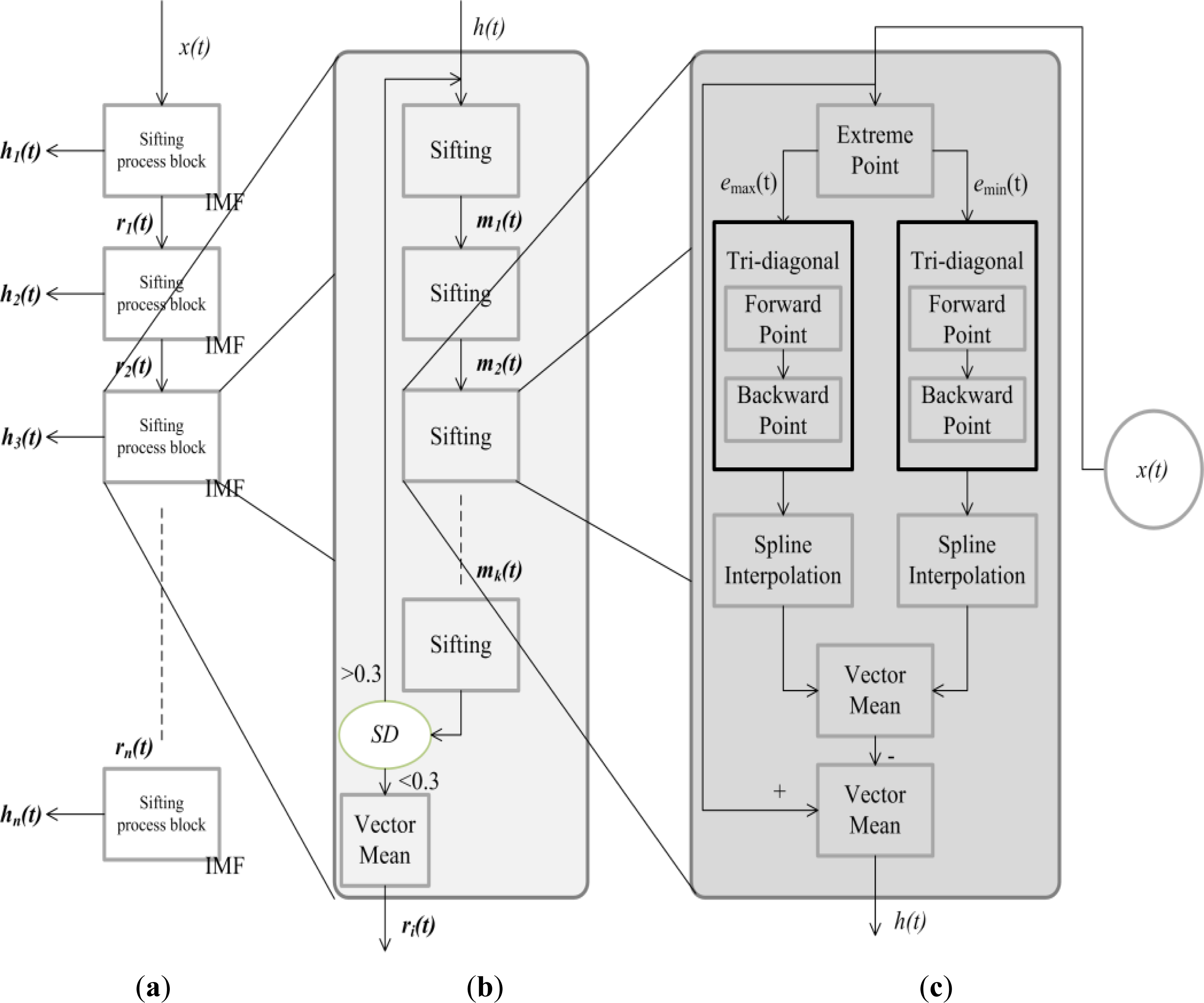
Figure 1 shows the operating procedures of EMD. First, in Figure 1(a), the signal x(t) is input and decomposed to n IMFs. Each IMF is calculated by the “k times” sifting process until the SD is less than 0.3 as shown in Figure 1(b). The sifting process (see Figure 1(c)) computes the difference between the signal x(t) and the mean of the maxima and minima envelopes.
Although the use of EMD has made significant contributions in many applications, its ability to handle signal-processing problems is still insufficient. Rilling and Flandrin [8,9] stated that EMD decomposition capability strongly depends on the frequencies and amplitudes, and the differences in both frequencies and amplitudes of two signals must be sufficient for EMD decomposition analysis. If the criteria for the differences between two signals are not met, the sifting process derives an IMF with a single tone modulated in amplitude instead of a superposition of two unimodular tones. This phenomenon is called the beat effect. To overcome the problem of mode mixing, Wu and Huang [10] proposed EEMD. A uniform distribution of white noise is added to signals before decomposition to reduce the effect of the mode mixing in the EMD process [20]. As a result, the EEMD method is capable of resolving both the issues of mode mixing and multi-dimensional computation [11].
For EEMD, the ratio of the added white noise and the number of signals in the ensemble must be predetermined. According to the number in the ensemble, different white noise wi(t) with the same amplitude is added N times to an original signal x(t) to generate N modified signals xi(t).
x i ( t ) = x ( t ) + w i ( t ) i = 1 , 2 , , N
Next, the EMD decomposition is performed on each modified signal xi(t). Assume the signal is decomposed into n units of IMF and one residue as a trend. Further, by the EEMD method, it will get N × n IMF signals and n trends rin(t). Then, xi(t) can be rewritten as:
x i ( t ) = j = 1 n h ij ( t ) + r i n ( t ) i = 1 , 2 , , N
To reduce the mode mixing, the EEMD method averages the result of the IMF set Hj(t) and the trend R(t) derived from EMD.
H j ( t ) = 1 N i = 1 N h ij ( t )     j = 1 , 2 , , n
R ( t ) = 1 N i = 1 N r in ( t )
The error in the decomposition caused by the added white noise is given by the following empirical formula of Wu et al. [10] for large amounts of data:
ɛ n = ɛ N
where N is the number of ensembles, ɛ is the amplitude of the added noise, and ɛn is the final standard deviation. According to this empirical formula, wi(t) can be obtained,
w i ( t ) = ɛ × noise ( t )
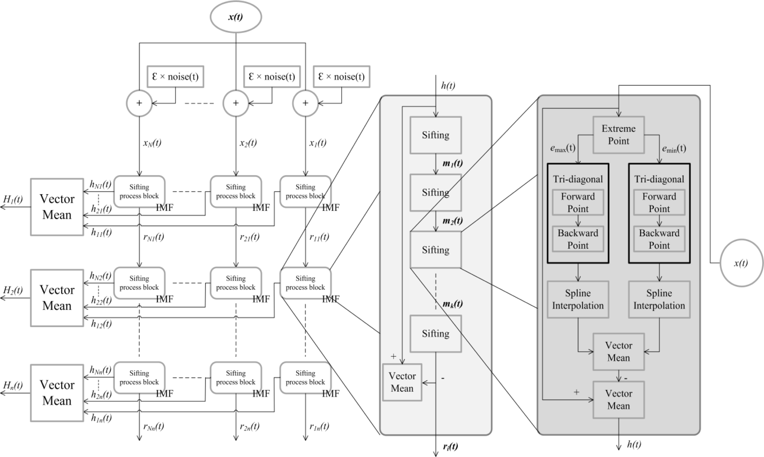
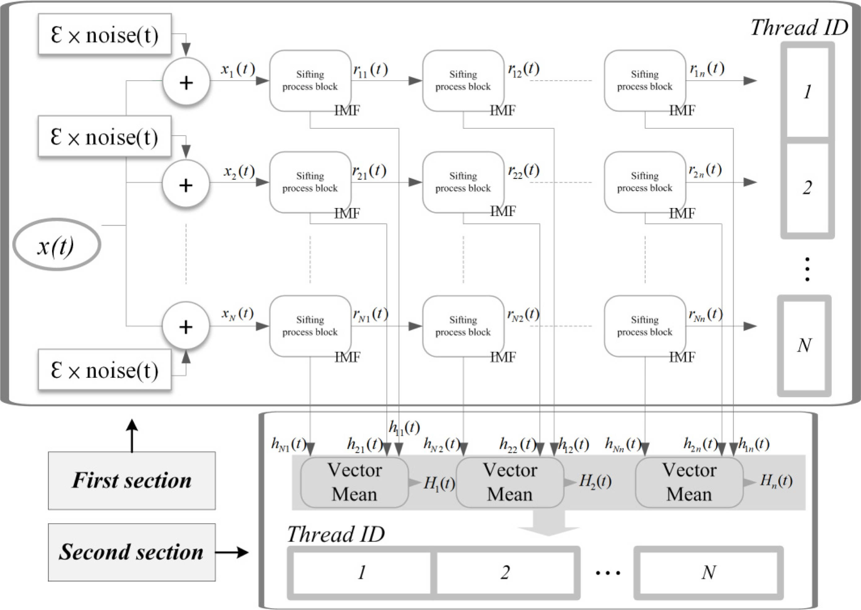
The EEMD process is shown in Figure 2. Comparing EEMD and EMD (Figure 1), the only difference is that EEMD needs to average N hj(t) to get each IMF, but EMD does not.

2.2. Spectral Angle Mapper

A measurement of the similarity of pixels is normally needed for spectral mapping, and the Spectral Angle Mapper (SAM) is a widely used as a spectral similarity metric in remote sensing [16]. In a scatter plot of pixel values from two bands of a spectral image, pixel spectra and target spectra will plot as points as shown in Figure 3. If a vector is drawn from the origin through each point, the angle between any two vectors defines the spectral angle between those two points. The SAM computes a spectral angle between the closest set of pixel spectra and the target spectra, si and sj.
SAM ( s i , s j ) cos 1 ( s i , s j s i s j ) = cos 1 ( l = 1 L s il s jl [ l = 1 L s il 2 ] 1 2 [ l = 1 L s jl 2 ] 1 2 )

2.3. Parallel Computing Implementations

In this research, the experiment adopts parallel-computing technology [18, 19] to speed up the EEMD. The EEMD method can be performed by a GPU developed by NVIDIA. The experiment divides EEMD into two sections. The first is to assign threads for computing each individual ith x(t), and to record an entire result of IMF hj(t) by iterative computation. For each input spectrum x(t), N additive Gaussian noises are randomly generated. Each thread processes one noisy spectrum and decomposes it into IMFs. The second is to compute in a parallel manner for a vector ensemble mean of the jth IMF from all threads (see Figure 4).

3. Experimental Results

The experimental data were provided by the United States Geological Survey (USGS) spectra library, where five minerals were chosen: actinolite, andradite, goethite, hematite and illite. Each material has four to 10 spectra (Figure 5). For each mineral, at least one spectrum is quite different from the others, which reduces the classification accuracy. The EEMD can extract the absorption feature to improve the accuracy.
To demonstrate the effectiveness of EEMD, the SAM was applied to the original and decomposed spectra by EMD and EEMD. Furthermore, a comparison of parameter settings for EEMD was also conducted, including noise standard deviation, number of signals in each ensemble average and number of accumulated IMFs.

3.1. SAM for Original Data

To assess the accuracy of discrimination between minerals, 2000 spectra of each material were simulated with additive white Gaussian noise having signal-to-noise ratio (SNR) 40, and spectral similarity was measured by SAM. Table 1 shows the similarity discrimination of these five minerals in contrast to the original spectra. The SAM values between pairs of five original spectra are 75.8%, 80%, 75%, 70.2% and 80%. The experiment examined the degree of accuracy by kappa coefficient [21]. The test result is reliable because the kappa coefficient is 0.7025.

3.2. SAM for EMD Decomposed Data

The EMD algorithm was applied to decompose the spectra into seven IMFs (Figure 6), and spectral similarity was measured by SAM for each IMF. From Table 2, the largest kappa coefficient occurs for the first IMF (0.6564) which is slightly less than that for the original data, while the worst kappa coefficient occurs for the sixth IMF (0.0079), which did not provide good discrimination.
Each IMF is ordered sequentially from higher frequencies to lower frequencies. Summation of all IMFs yields the original data. Because we compared the absorption feature of each IMF with the original spectra, the wavelength of the absorption feature can be estimated. Since this feature is distributed through several IMFs, combining a set of IMFs should enhance the absorption features. The accumulation of IMFs is shown in Figure 7, and the absorption features are clearly observed.

3.3. SAM for EEMD Decomposed Data

EEMD was employed to overcome the drawback of mixing modes in EMD. Several parameters have to be determined to initialize EEMD, including noise standard deviation (Nstd), number of signals in each ensemble average (N) and number of accumulated IMFs.
First, the accuracy of performance for each number of signals in the ensemble average was analyzed by kappa coefficient (Table 3). The noise standard deviation was selected from 0.1–0.9, and the numbers, N, for the ensemble averages were 10, 50, 80, 100, 500 and 1,000. When N = 1, EEMD is identical to EMD. The experimental results show a stable kappa value when N exceeds 100 (Figure 8). Therefore, considering the efficiency of the algorithm, N was set to be 100 for EEMD.
Secondly, the noise standard deviation needs to be determined. From Table 4, N for the ensemble average is 100, the noise standard deviation (Nstd) is from 0.1–0.9. The simulated data contain additive white Gaussian noise with SNR = 20, 30 and 40. The results show that the kappa coefficients are over 0.7511 and 0.8688 for the third and fourth IMF, respectively, for all Nstd from 0.1–0.9 and SNR 40. Significant improvements are obtained with the third or fourth IMF with EEMD alone compared with the accuracy of original data (0.7025). The maximum kappa value is 0.9771 when Nstd = 0.2, SNR = 40 for the fourth IMF. Therefore, if the spectral estimate has high SNR, with noise standard deviation less than 0.2, EEMD performs well.
Finally, the number of accumulated IMFs was analyzed. Several IMFs contain absorption features, so that the accumulation of a set of IMFs should enhance the classification accuracy (Figure 6). To accumulate IMFs, the absorption features must be clearly identified. In this experiment, the number of signals in the ensemble average was set as 100 to optimize, as closely as possible, the tradeoff between noise reduction and efficiency. EEMD was applied to various SNRs and noise standard deviations. Table 5 shows the classification accuracy using SAM values of the accumulated IMFs: IMF 1–2, IMF 1–3, IMF 1–4, IMF 1–5, IMF 1–6. The results show that the kappa coefficients are over 0.7556 and 0.9224 for IMF 1–3 and IMF 1–4, respectively, for all Nstd and SNR 40. They also indicate that EEMD provides further improvements for the fourth IMF compared with the third IMF. The highest kappa value is 0.9909 when Nstd = 0.2, SNR = 40 for IMF 1–4.
Furthermore, the kappa coefficient decreased when Nstd > 0.5, indicating that the classification accuracy was also reduced. If the spectra have low SNR, both the number of IMFs and the Nstd need to be increased to achieve an acceptable performance. On the other hand, with high SNR, no matter how many IMFs are used, the classification performs well when Nstd < 0.5. The stable performance appears with IMF 1–5 and Nstd = 0.5, the kappa coefficient is 0.8051, 0.9455, and 0.9830. For higher classification accuracy and computational efficiency, it suggests EEMD with N = 100, Nstd = 0.2–0.5 and accumulation of IMF 1–4 or IMF 1–5.

3.4. EEMD Speedup by GPU

The computation environments are shown in Table 6. The proposed algorithm was developed to run on NVIDIA Tesla C1060 GPU via CUDA, and was compared with its CPU serial code on Intel Xeon 5504 with Linux, and Intel i5-2400 with Windows 7. CUDA (Computer Unified Device Architecture) is a parallel-computing platform and programming model created by NVIDIA and implemented by the GPUs that they produce. Table 7 shows the performance of EEMD in four different processing environments and computer language. For performance comparison, the numbers of test samples (N) are chosen from 500 to 3,000. In PC environment, the computing time is approximately proportional to the number of samples and C/C++ language is about five times faster than Matlab. Comparing the environments using C language, the cluster architectures can further improve the performance. The computational performances have 15 and 60 times improvement with quad-core CPU and GPU, respectively, when N exceeds 2,000. It is worth noting that the 240-core GPU is not efficiently utilized with a small sample size—when N = 500—with only a 30 time improvement for GPU compared to a PC environment.

4. Conclusions

Empirical mode decomposition (EMD), a fully data-driven method for decomposing signals (Huang et al. [7]), is excellent for extracting nonlinear characteristics of signals. Additionally, EEMD outperforms EMD by accommodating noise and avoiding the beat effect. We proposed a two-stage process for spectral similarity measurement; first, adopt EEMD to generate a series of IMFs and then accumulate a set of IMFs for enhancing absorption features; secondly, use the SAM technique for hyperspectral image classification. The experimental results show that EEMD-decomposed hyperspectral signals can enhance discrimination ability. The IMFs also indicate the absorption features of spectra, and the accumulated IMFs can improve absorption characteristics. Our study also overcame two drawbacks of EEMD; the algorithm is time-consuming and several parameters have to be determined before processing. To overcome the first drawback, we propose parallel processing with GPU architecture to decompose spectral data. The performance analysis shows that GPU can significantly reduce the computing time for EEMD. Our insights into selecting three key parameters (noise standard deviation, number of signals in ensemble averages, and the number of accumulated IMFs for EEMD) assist in overcoming the second drawback.

Acknowledgments

The authors would like to express their appreciation to United States Geological Survey for providing spectral library used in this study.

Author Contributions

Hsuan Ren and Hung-Ming Kao provided the background knowledge of EMD and EEMD to decompose 1-dimensional signal into IMFs. Hsuan Ren, Yung-Ling Wang and Hung-Ming Kao conceived the research topic of using EMD and EEMD to decompose spectrum to improve the classification performance. Min-Yu Huang, Yung-Ling Wang and Hung-Ming Kao implemented EMD and EEMD in various computational environments for comparison. Min-Yu Huang and Yung-Ling Wang conducted the data acquisition, analysis, literature review, tables, figures and preparation of manuscript. Yang-Lang Chang, Hsuan Ren and Hung-Ming Kao not only participated in methods selection and discussions but also in editing and revisions of the paper. Hsuan Ren, Yang-Lang Chang, Yung-Ling Wang and Hung-Ming Kao also had provided the background knowledge and performed editing in the revised manuscript.

Conflicts of Interest

The authors declare no conflict of interest.

References

  1. Chang, C.I. Hyperspectral Imaging: Techniques for Spectral Detection and Classification; Kluwer Academic/Plenum Publishers: New York, NY, USA, 2003. [Google Scholar]
  2. Carvalho, O.A., Jr.; Guimaraes, R.F.; Gillespie, A.R.; Silva, N.C.; Gomes, R.A.T. A new approach to change vector analysis using distance and similarity measures. Remote Sens 2011, 3, 2473–2493. [Google Scholar]
  3. Kamal, M.; Phinn, S. Hyperspectral data for mangrove species mapping: A comparison of pixel-based and object-based approach. Remote Sens 2011, 3, 2222–2242. [Google Scholar]
  4. Keshava, N. Distance metrics and band selection in hyperspectral processing with application to material identification and spectral libraries. IEEE Trans. Geosci. Remote Sens 2004, 42, 1552–1565. [Google Scholar]
  5. Hecker, C.; van der Meijde, M.; van der Werff, H.; van der Meer, F.D. Assessing the influence of reference spectra on synthetic SAM classification results. IEEE Trans. Geosci. Remote Sens 2008, 46, 4162–4172. [Google Scholar]
  6. Van der Linden, S.; Waske, B.; Hostert, P. Towards an Optimized Use of the Specral Angle Space. Proceedings of the 5th EARSeL Workshop on Imaging Spectroscopy, Bruges, Belgium, 23–25 April 2007; pp. 1–5.
  7. Huang, N.E.; Shen, Z.; Long, S.R.; Wu, M.C.; Shih, H.H.; Zheng, Q.; Yen, N.C.; Tung, C.C.; Liu, H.H. The empirical mode decomposition and the Hilbert spectrum for nonlinear and non-stationary time series analysis. Proc. R. Soc. A 1998, 454, 903–999. [Google Scholar]
  8. Flandrin, P.; Rilling, G.; Goncalvés, P. Empirical mode decomposition as a filter bank. IEEE Signal Process. Lett 2004, 11, 112–114. [Google Scholar]
  9. Rilling, G.; Flandrin, P.; Goncalves, P. On Empirical Mode Decomposition and its Algorithm. Proceedings of the 6th IEEE/EURASIP Workshop on Nonlinear Signal and Image Processing (NSIP’03), Grado, Italy, 8–11 June 2003; pp. 8–11.
  10. Wu, Z.; Huang, N.E. Ensemble empirical mode decomposition: A noise-assisted data analysis method. Adv. Adapt. Data Anal 2009. [Google Scholar] [CrossRef]
  11. Wu, Z.; Huang, N.E.; Chen, X. The multi-dimensional ensemble empirical mode decomposition method. Adv. Adapt. Data Anal 2009, 1, 339–372. [Google Scholar]
  12. Li, X.; Li, X.B.; Huang, Z.Y. Signal extraction using ensemble empirical mode decomposition and sparsity in pipeline magnetic flux leakage nondestructive evaluation. IEEE Trans. Rev. Sci. Instrum 2009, 80. [Google Scholar] [CrossRef]
  13. Linderhed, A. Image empirical mode decomposition: A new tool for image processing. Adv. Adapt. Data Anal 2009, 1, 265–294. [Google Scholar]
  14. Demir, B.; Ertürk, S. Empirical mode decomposition of hyperspectral images for support vector machine classification. IEEE Trans. Geosci. Remote Sens 2010, 48, 4071–4084. [Google Scholar]
  15. Zhang, M.; Shen, Y. Ensemble empirical mode decomposition for hyperspectral image classification. Adv. Adapt. Data Anal 2012, 4. [Google Scholar] [CrossRef]
  16. Erturk, A.; Gullu, M.K.; Erturk, S. Hyperspectral image classification using empirical mode decomposition with spectral gradient enhancement. IEEE Trans. Geosci. Remote Sens 2013, 51, 2787–2798. [Google Scholar]
  17. Xu, Y.P.; Hu, K.N.; Han, J.X. Classification based on the EMD of hyperspectral curve. Proc. SPIE 2007, 6795. [Google Scholar] [CrossRef]
  18. Chang, L.W.; Lo, M.T.; Anssari, N.; Hsu, K.H.; Huang, N.E.; Hwu, W.M.W. Paralle implementation of multi-dimensional ensemble empirical mode decomposition. IEEE Trans. Acoust. Speech Signal Process. (ICASSP) 2011. [Google Scholar] [CrossRef]
  19. Chen, D.; Li, D.; Xiong, M.; Bao, H.; Li, X. GPU-aided ensemble empirical mode decomposition for EEG analysis during anesthesia. IEEE Trans. Inf. Technol. Biomed 2010, 14, 1417–1427. [Google Scholar]
  20. Wu, Z.; Huang, N.E. A study of the characteristics of white noise using the empirical mode decomposition method. Proc. R. Soc. A 2004, 460, 1597–1611. [Google Scholar]
  21. Carletta, J. Assessing agreement on classification tasks: The kappa statistic. J. Comput. Linguist 1996, 22, 249–254. [Google Scholar]
Figure 1. The procedure for Empirical Mode Decomposition (EMD). (a) Main flow; (b) Calculation of IMF; (c) The sifting process.
Remotesensing 06 02069f1
Figure 2. The procedure for Ensemble Empirical Mode Decomposition (EEMD) processing.
Remotesensing 06 02069f2
Figure 3. Concept of Spectral Angle Mapper (SAM).
Remotesensing 06 02069f3
Figure 4. The Graphics Processing Unit (GPU) architecture of EEMD.
Remotesensing 06 02069f4
Figure 5. Spectral reflectance results for five minerals.
Remotesensing 06 02069f5
Figure 6. The spectra of Intrinsic Mode Functions (IMFs) by EMD for Actinolite.
Remotesensing 06 02069f6
Figure 7. Spectra of accumulations of IMFs from 1–6.
Remotesensing 06 02069f7
Figure 8. Kappa value vs. N and Nstd for IMF1 with SNR = 30.
Remotesensing 06 02069f8
Table 1. Similarity discrimination rates on the experimental samples of five minerals vs. USGS spectral library.
ActinoliteAndraditeGoethiteHematiteIllite
Actinolite75.8%0%0%0%0%
Andradite0%80%25%29.4%20%
Goethite0%0%75%0%0%
Hematite20%20%0%70.2%0%
Illite4.2%0%0%0.4%80%

Kappa value0.7025
Table 2. The similarity discrimination rate for the EMD process on the samples of five minerals.
ActinoliteAndraditeGoethiteHematiteIlliteKappa
IMF 1100%60%75%58.3%80%0.65640
IMF 2100%60%25%50%80%0.52632
IMF 328.6%80%0%75%60%0.46137
IMF 40%40%0%75%40%0.34278
IMF 5100%20%0%25%0%0.02623
IMF 60%60%0%16.7%0%0.00794
IMF 733.3%40%0%25%80%0.22132
Table 3. Kappa value vs. N and Nstd for IMF 1 with SNR = 30.
IMF 11102550801005001000
0.10.17950.11840.11900.11850.11010.11160.10940.1098
0.20.12590.12910.13690.11610.11290.11030.11050.1109
0.30.09180.12400.12650.12250.11980.11540.11600.1154
0.40.04050.10640.11590.11940.11460.11140.11380.1130
0.50.08500.10280.10910.11890.11000.11190.11210.1133
0.60.07600.09840.10950.11450.11010.11090.11200.1134
0.70.05190.12480.09880.10560.10580.11080.11240.1134
0.80.04580.05260.08810.10110.10180.10880.11100.1148
0.90.02590.04450.05630.08300.09360.09850.10590.1074
Table 4. Kappa values of IMF1∼7 in SNR = 20∼40 vs. Nstd under N = 100.
Nstd0.10.20.30.40.50.60.70.80.9

N = 100
IMF 1SNR = 200.10510.11280.11310.11510.11460.11140.11100.10960.1098
SNR = 300.11160.11030.11540.11140.11190.11090.11080.10880.0985
SNR = 400.56130.50680.49200.47100.45700.43980.42840.41490.4034

IMF 2SNR = 200.19350.20660.21830.22400.22360.21990.21800.22140.2145
SNR = 300.15880.15400.14860.14210.13700.13510.12940.12710.1293
SNR = 400.71730.65000.59600.56780.53360.51580.49740.47990.4515

IMF 3SNR = 200.31250.36780.38500.39240.40050.39530.38480.37400.3764
SNR = 300.35110.35010.33810.33590.34140.33630.33710.33360.3343
SNR = 400.83850.86310.85050.82530.80340.78850.77080.75960.7511

IMF 4SNR = 200.48140.57850.60630.62800.62350.61510.59660.59490.5863
SNR = 300.50610.49360.46700.47490.45130.44300.42910.42930.4109
SNR = 400.87910.97710.95310.95350.92200.91910.90350.89450.8688

IMF 5SNR = 200.34750.52110.61990.63210.66190.67330.66360.67550.6873
SNR = 300.58550.65710.66810.66280.66550.66000.65300.64960.6473
SNR = 400.61330.77640.79950.82210.84140.86530.86960.88000.8865

IMF 6SNR = 200.34290.37300.55740.56500.58580.60300.60390.59630.5866
SNR = 300.53190.54860.72000.72580.74380.77190.75080.75210.7618
SNR = 400.30210.48330.50250.55710.58350.62210.63660.65140.6636

IMF 7SNR = 200.37300.45400.45810.46430.45540.42960.41960.42910.3998
SNR = 300.48580.60790.64130.66750.68660.69480.67310.67830.6276
SNR = 400.49640.50140.49910.52250.53390.53160.51860.51250.4715
Table 5. Kappa values of the accumulated IMF (1–2 to 1–6) in SNR = 20∼40 vs. Nstd when N = 100.
Nstd0.10.20.30.40.50.60.70.80.9

N = 100
IMF 1–2SNR = 200.22430.23150.23750.23480.23430.23280.23210.22810.2231
SNR = 300.46610.45260.43860.42850.41990.41400.40750.40090.3951
SNR = 400.74480.68680.63690.62080.58110.56080.54360.52760.5276

IMF 1–3SNR = 200.40110.41110.40950.40160.39650.39210.38630.38080.3818
SNR = 300.71790.72200.70560.69460.68150.67010.65990.64660.6375
SNR = 400.89100.87260.85260.83350.81540.80000.78410.76680.7556

IMF 1–4SNR = 200.60040.63740.64330.64190.63800.62660.61430.60850.5965
SNR = 300.84730.84380.84680.85580.84810.84100.83080.82560.8174
SNR = 400.98550.99090.98330.98440.97490.96340.95100.94010.9224

IMF 1–5SNR = 200.71580.79110.79940.79880.80510.80380.79750.79390.7923
SNR = 300.92010.93430.93740.94400.94550.94600.94040.94650.9439
SNR = 400.93780.94300.96450.97540.98300.98640.99090.99240.9945

IMF 1–6SNR = 200.81640.81300.80200.81080.80740.81160.80150.80280.8041
SNR = 300.89840.88050.85390.87380.86360.87160.86010.87890.8760
SNR = 400.90830.88680.84730.88690.87240.88450.99090.88750.8873
Table 6. Computation Environments.
PCCluster
CPUCPUGPU
Operating SystemWindows 7 SP1Debian GNU/Linux 6.0.2
PlatformIntel i5-2400Intel Xeon 5504 (Quad-core)Tesla c1060 (240 cores)
Clock rate3.1 GHz2.0 GHz1.3 GHz
MemoryDDR3 4G × 2DDR3 2G × 6DDR3 4G
LanguageMatlab 2008aVS2008-C/C++Linux-CLinux-C&CUDA
Table 7. The performance of EEMD in various computational environments (values are in seconds).
NMatlab 2008aVS2008-C/C++Linux-CLinux-C&CUDA
50034,1276240423.03207.59
100066,57413,073846.19283.22
150099,65019,1881268.53345.29
2000132,62424,7571692.13408.37
2500165,57530,9662112.62561.02
3000199,10937,0972548.61684.97

