Article

Forest Variable Estimation Using Radargrammetric Processing of TerraSAR-X Images in Boreal Forests

Department of Forest Resource Management, Swedish University of Agricultural Sciences, SE-901 83 Umeå, Sweden
*
Author to whom correspondence should be addressed.
Remote Sens. 2014, 6(3), 2084-2107; https://doi.org/10.3390/rs6032084
Submission received: 23 December 2013 / Revised: 17 February 2014 / Accepted: 24 February 2014 / Published: 7 March 2014

Abstract

:
The last decade has seen launches of radar satellite missions operating in X-band with the sensors acquiring images with spatial resolutions on the order of 1 m. This study uses digital surface models (DSMs) extracted from stereo synthetic aperture radar images and a reference airborne laser scanning digital terrain model to calculate the above-ground biomass and tree height. The resulting values are compared to in situ data. Analyses were undertaken at the Swedish test sites Krycklan (64°N) and Remningstorp (58°N), which have different site conditions. The results showed that, for 459 forest stands in Remningstorp, biomass estimation at the stand level could be performed with 22.9% relative root mean square error, while the height estimation showed 9.4%. Many factors influenced the results and it was found that the topography has a significant effect on the generated DSMs and should therefore be taken into consideration when the stand level mean slope is above four degrees. Different tree species did not have a major effect on the models during leaf-on conditions. Moreover, correct estimation within young forest stands was problematic. The intersection angles resulting in the best results were in the range 8–16°. Based on the results in this study, radargrammetry appears to be a promising potential remote sensing technique for future forest applications.

1. Introduction

There is a significant international interest regarding accurate estimations of carbon sequestration [14]. Sweden is well placed for undertaking research into forest variables at both small scale (tree-level) and large scale (national level) due to its significant areas of forest land (28.1 million ha) and its well-established research structure. The Swedish National Forest Inventory (NFI) carries out an inventory on about 11,000 field plots [5], annually, in Sweden. In combination with remote sensing data from, e.g., airborne laser scanning (ALS), accurate estimations of the current state of the forest can be obtained [6]. It is established that ALS can provide very accurate estimates of heights and forest related variables [79] and can be used for creating digital terrain models (DTMs) to describe ground elevation. However, the airborne platform for ALS is relative expensive and it can, therefore, not be used for frequent inventories, e.g., on an annual basis over large areas. Satellite-borne sensors can cover large areas and often have very short repeat periods, commonly within one to two weeks. Optical satellite sensors can suffer from problems with cloud cover, especially in regions around the equator, but also at northern latitudes. Satellite radar sensors, however, with their active techniques, overcome this issue and currently seem to be one of the more attractive options [10] for carrying out frequent remote sensing of forests. From radar data a digital surface model (DSM) can be calculated, coinciding with the DTM in open regions while also describing the upper vegetation canopy in vegetated areas. As is the case in many countries, the ground elevation is well known in Sweden thanks to extensive ALS scans. The difference between the DSM and the DTM will be referred to as canopy height model (CHM) and contains information related to the forest above-ground biomass (AGB) and basal area-weighted tree height (H).
Synthetic aperture radar (SAR) acquires images with backscatter intensity, phase, and finally, also the distance, based on the time for the transmitted signal to return to the receiver. The last decade has seen a dominance of interferometric SAR (InSAR) and polarimetric InSAR (PolInSAR), both making use of the phase and its polarization of the radar signal, while older techniques historically used for optical imagery have received less attention. With the launch of the German TerraSAR-X and the Italian COSMO-SkyMed satellites, in 2007, radargrammetric processing (first used in the 1960s, [11]) has taken an important step forward. Both these satellites have spatial resolutions on the order of 1 m [12], offer various look angles, and have accurate geolocation. This geolocation accuracy was reported to be on the order of less than 1 m [13] and independent studies have later verified this [14,15], e.g., by using corner reflectors and the boundary condition that they are projected on known elevations. Raggam et al. [16] could not fully validate this accuracy, but, nevertheless, concluded an overall accuracy of about 2 m. They also concluded that sensor model adjustments were sensitive with regards to Multi Looked Ground-Range Detected (MGD) products and that stereo mapping is a very challenging objective, in particular over forested or other terrain with high radiometric variability.
Radargrammetry uses the stereoscopic viewing well-known from optical photogrammetry, applied to radar images. Instead of the optical wavelengths, the aforementioned satellite sensors operate in the X-band with about 0.03 m wavelength. Radargrammetry, in contrast to InSAR or PolInSAR, uses the backscatter intensity, similar to the optical case, to form images used for stereo matching. The backscattered intensity images need to be acquired from different incident angles (causing intersection angles) to possess the inherent disparities of an object appearing slightly different from different directions. The measured parallaxes between the two images are directly correlated to the terrain elevation. In the case of forest vegetation, X-band signals are unlikely to reach the ground, but instead to slightly penetrate the upper canopy down to different depths depending on many factors such as transmissivity, tree density, tree species, and temperature.
In general, the observed parallaxes can be estimated with a higher degree of accuracy as the angle of intersection increases (as the stereo exaggeration factor increases). However, in contrast to this, it is required that the images are as similar as possible in order to improve the image matching which is best achieved with small intersection angles. It was concluded in [17] that the larger intersection angle, the more the quality of the stereoscopic fusion deteriorates and this becomes even more pronounced with high-relief terrain. The principal parameters influencing the DSM accuracy the most are the type of the relief and its slope. The common compromise has been to use same-side stereo-pairs with intersection angles of about 8–20° [1719]. This will generally result in reasonable geometric and radiometric disparities and the data will be suitable for the radargrammetric processing.
Many studies have been performed with TerraSAR-X data, but the majority have focused either on the accuracy of the elevation reconstruction, the geolocation or other technical properties, describing it more as an instrument comparative with, e.g., ALS. Some of the earliest studies deriving forest related variables from TerraSAR-X data are described in [2022]. They found that the accuracy of the derived DSMs were very high over bare ground while regions of forest were underestimated in the range of 25%–35% compared to the real canopy height, with an average underestimation of 27%. They also concluded that additional experiments over different types of forest are needed to establish if this underestimation would be reduced on a large scale. These early forest studies were extended in [23]. As mainly dense stands of deciduous trees were used, it was also stated that the canopy height underestimation was expected to be larger for coniferous trees and for clearer stands. No seasonal effects (frozen/unfrozen) or the influence of weather conditions could be studied as all images used in the study were acquired during April–June and no weather differences were present. This was also the case in [24] where the authors carried out Random Forest evaluation of forest using 109 field plots with 8 m radius, using only spring-time images. They found that the forest stem volume could be predicted with 34.0% relative root mean square error (RMSE) and the mean forest canopy height with 14.0%. Overall, the authors concluded that the influences of tree species, seasonal effects, and weather conditions have to be studied further. A further study [25] from primarily the same authors utilized the same field and SAR data, but investigated plot-level estimations of AGB and stem volume compared to ALS estimates. The authors concluded that radargrammetry is a promising technique for this and that AGB and stem volume could be estimated with 29.9% and 30.2% relative accuracy in comparison with 21.9% and 24.8% for ALS. They also concluded that further studies on radargrammetry for large-area mapping are needed.
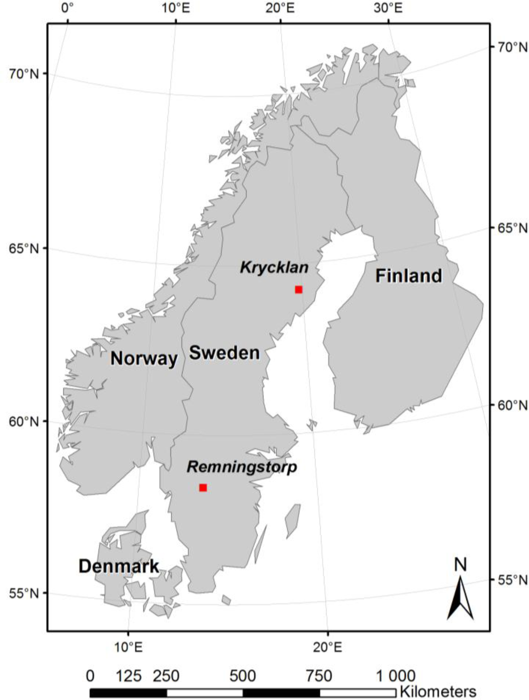
The study presented here puts a larger emphasis on forestry conditions and less on the technical aspects, trying to cover as many of the previously addressed issues as possible; i.e., using pre-stratified forest stand maps with a variety of stand sizes, ALS reference data combined with manually measured field plots, and different test sites with varying site conditions containing different tree species. The different test sites facilitate an analysis of the influence of the topography. The overall objective of thisstudy is to evaluate the potential of using radargrammetry with TerraSAR-X images for estimating basal area-weighted tree height and the strongly related variable above-ground biomass at stand level.

2. Test Sites and Materials

2.1. Field Data

For this study two Swedish test sites with different site conditions have been used (Figure 1). The first site is the Krycklan river catchment area located in northern Sweden (Lat. 64°16′N, Long. 19°46′E). The catchments 7470 ha are divided into 1751 stands. Of these, 6780 ha (1380 stands) are forested. Only 754 of the 1751 stands were covered by the TerraSAR-X spotlight (SL) data. These 754 stands ranged from 0.5–54.2 ha in size. For the entire test site, the prevailing tree species were Scots pine (Pinus sylvestris; 49%, mainly in dry upslope areas), Norway spruce (Picea abies; 35%, mainly in wetter, low-lying areas), and birch (Betula pendula and Betula pubescens; 15%, in the riparian forest along larger streams). In the lower reaches of the catchment, larger streams have deeply incised channels carving through fine-grained floodplain sediments. The region is hilly with elevations between 125 m and 350 m above sea level and slopes up to 61° at pixel level (the slope calculated from an 8 neighboring environment of DTM pixels, [26]).
In total, 110 field plots with 12 m radius (Figure 2a) were randomly distributed in the central parts of the study area within the same ALS strips used in [27]. The entire test site was scanned, but additional cross strips were distributed to geometrically bind together the total ALS scans, resulting in a higher total pulse density within these strips, where the 110 field plots were distributed. The tree height distribution of the covered plots represents the entire known height range from field measurements. All tree species were also present on this test site. The plots were surveyed during August 2008 and the positions of the field plot centers were measured using a post-processed Differential Global Positioning System. Trees with a diameter at breast height (DBH) ≥ 0.04 m were measured using a caliper and the species were recorded. For a random sub-sample of trees with inclusion probability proportional to basal area, the tree height was also measured using a hypsometer. The number of trees for which the height was measured was 299, which corresponds to 5.1% of the calipered trees. Based on the trees with diameter and height measures, multiple linear regression models were constructed based on three tree classes: pine, spruce, and deciduous. Equation (1) illustrates the regression model used to model the tree height for all calipered trees, where hi is the tree height and DBHi is the DBH, of tree i.
ln ( h i ) = α + β 1 DBH i + β 2 ln ( DBH i )
the best diameter/height correlation was found for spruce trees, but all relative RMSEs lay between 13.3% and 25.8%. Equation (2) illustrates the definition used for calculating the relative RMSE, where and Y are the estimated and reference metric (AGB or H) for stand i and n stands in total.
RMSE % = i = 1 n ( Y ^ i Y i ) 2 / n i = 1 n ( Y i ) / n 100
The H was calculated for each plot. The AGB was calculated using the allometric equations of [28] with DBH as input variable and then aggregated to plot level.
Additionally, 31 of the previously mentioned forest stands were inventoried for the BioSAR 2008 campaign [29]. The size of the selected stands varied between 2.4 ha and 26.3 ha. In the selected stands, field plots were distributed with a systematic spacing of 50 m to 160 m, depending on the size of the area. The spacing in each stand was determined with the aim of obtaining 10 plots in each stand. The resulting number of plots for all stands varied between 8 and 13, with an average of 10 plots per stand. In total, 311 field plots were allocated within the 31 stands visited. On the plots with 10 m radius, all trees with a DBH ≥ 0.04 m were calipered and the species registered. On randomly selected sample trees (selected with their probability proportional to their basal area) height and age were also measured. On average, 1.5 sample trees were selected per plot. For this additional field inventoried data set, the stands covered by the TerraSAR-X SL images were limited to 20, ranging from 0.7 ha to 26.1 ha in size.
The second test site, Remningstorp, is located in southern Sweden (Lat. 58°30′N, Long. 13°40′E) and comprises about 1200 ha forest divided into 531 stands. The prevailing tree species are Norway spruce, Scots pine and birch. It is a rather flat region with moderately varying ground elevations between 120 m and 145 m above sea level. Field plot data for the Remningstorp test site were collected in a previous study [30]. In total, 212 field plots (Figure 2b) with 10 m radius were allocated over the estate using a 200 m grid spacing. All trees on each plot with a DBH ≥ 0.04 m were calipered. In addition, tree heights were measured on a random sub-sample of trees at each plot. The 212 plots were surveyed during September and October 2010.
All field data (for both test sites) were collected in the Rikets Nät 90 (RT90)/Bessel 1841 coordinate system and then transformed to the Universal Transverse Mercator (UTM) zone 33N/World Geodetic System 1984 (WGS84) coordinate system to match the other data sources.

2.2. Stand Delineation

The delineation for the Krycklan test site (Figure 2a) was undertaken in 2008 by a professional interpreter using a combination of aerial photographs. For the western parts, scanned IRF photographs (covering the image bands infra-red, red, and green) from the analog RC30 15/4 Uag-S 13215 camera captured at a flight altitude of 4600 m above ground level (corresponding to a pixel size of 0.5 m) from 2004 were used. For the eastern parts, stereo-pair aerial photographs from the Z/I DMC digital camera, captured at a flight altitude of 4800 m above ground level (corresponding to a pixel size of 0.5 m) from 2007 were used. The delineation for the Remningstorp test site (Figure 2b) was undertaken in 2004 by a professional interpreter using stereo-pair aerial photographs from the Z/I DMC digital camera, captured at a flight altitude of 4800 m above ground level (corresponding to a pixel size of 0.5 m). Stands smaller than 0.5 ha were removed in order to avoid inclusion of too small stands in the analysis.

2.3. ALS Data

For both test sites ALS data, field plot inventory data and radar images were available for the same years. The ALS of the Krycklan catchment as part of the BioSAR 2008 campaign [29] was performed on 5–6 August 2008, with the TopEye MkII system (S/N 425), a laser wavelength 1064 nm, beam divergence 1 mrad, approximately 4 ns pulse width, and a pulse repetition frequency of 50 kHz. The system was mounted on a helicopter flying at an altitude of 500 m above ground level for the main strips and 250 m above ground level for the cross strips. Approximately 70 km2 were covered using an average density of approximately 5 returns per square meter in the main strips and 15 returns per square meter in the cross strips. The first and last returns were saved for each laser pulse. The coordinate system used was RT90, but the data were transformed to UTM-33N/WGS84 in order to match the other data sources.
The ALS scanning of the Remningstorp estate was performed on 29 August and 9 September 2010 [30]. The acquisitions were carried out using the helicopter-mounted TopEye MkIII system (S/N 700), a laser wavelength of 1550 nm, beam divergence ≤ 0.5 mrad, and an approximate pulse width of 3 ns. The scanner system uses a rotating polygon mirror with four mirror facets. A pulse repetition frequency of 160 kHz was used and the number of targets detected from each emitted pulse can be programmed separately. The density was at least 10 returns per square meter from 400 m altitude and at least 30 returns per square meter from 200 m altitude above ground level. The data were stored in the UTM-33N/WGS84 coordinate system. The two ALS systems are owned and operated by the company Blom Sweden AB.
In addition to the aforementioned ALS scans, the Swedish National Land Survey (Lantmäteriet) has undertaken a planned six-year project, since 2009, with the goal of scanning entire Sweden in order to generate an accurate DTM which, as only minor changes in the terrain are expected, should remain stable for the foreseeable future [31]. This ALS scan is airplane based with at least 0.5 returns per square meter and the average height error in all terrain types (asphalt, coniferous forest, deciduous forest, clear-cut forest, grass surface, bog, and grassland) is about 0.25 m. These ALS data were used as reference for both test sites and the coordinate system was SWEREF99TM that is based on UTM-33N (covering most of Sweden) and then extended to the adjacent UTM zones (32 and 34) in the western and eastern parts. The height reference system was Rikets Höjdsystem 2000 (RH2000) with the zero level defined by Normaal Amsterdams Peil (NAP), used in many European countries. By using the geoid heights obtainable from Lantmäteriet, a bi-linear interpolated correction raster was derived to calculate the ellipsoidal DTM raster, which was finally used.

2.4. Raster Data Modeling

The collected ALS data were related to the field plots for each test site through multiple linear regression models and evaluated through cross-validation to create AGB and H rasters used as reference data (denoted ALS estimated biomass/height) for the radargrammetry estimations. For Krycklan, Equations (3) and (4) were used, while for Remningstorp, the creation was performed and described in [32]. Equation (3) illustrates the regression model used to relate AGB to ALS data, where p60 is the 60th ALS percentile and VR the vegetation ratio for plot i.
ln ( AGB i ) = α + β 1 ln ( p 60 i ) + β 2 ln ( VR i )
Equation (4) illustrates the regression model used to relate H to ALS data, where p95 is the 95th ALS percentile and VR the vegetation ratio for plot i.
ln ( H i ) = α + β 1 ln ( p 95 i ) + β 2 ln ( VR i )
The rasters were generated with a 10 m pixel size to give a pixel area on the same order as the area of the field plots, and because the derived ALS metrics were available with this pixel size. The raster properties are described in Table 1.

2.5. TerraSAR-X Data

TerraSAR-X data were acquired for Krycklan in stripmap (SM) mode on 11 October 2008, and in SL mode on 16–17 October 2008. They were all delivered as Level 1b (L1b) products in the form of MGD images and are listed in Table 2. For Remningstorp, the images were acquired in high-resolution spotlight (HS) mode on 22 and 27 August, and 2 and 7 September 2010. These were L1b products delivered as Single Look Slant Range Complex images, giving different azimuth and range ground sampling distances (GSD), and are listed in Table 3. All TerraSAR-X images were collected the same years as their respective field data were surveyed, which should result in negligible temporal differences both within the satellite image pairs, to the ALS data, and between satellite data and the field surveyed data. The images for Krycklan were acquired in both single and dual polarization mode but only the HH polarization was consistently used, even when other polarizations were available in one or the other image. For Remningstorp all images were acquired in single polarization mode. In Tables 2 and 3, both, the resolutions (describing the sensor slant range and azimuth resolutions) and the GSD, are listed for the images. A more detailed description of how GSD and the resolution are related is described in [33].
The SL scene KR2 for Krycklan unfortunately did not cover the entire test site and therefore only 43% of the available stands could be used for the modeling and evaluation. In order to facilitate comparisons of the data, all images from Krycklan were cut to cover the same region as the smallest SL image. An example of the differences in information content linked to image quality is illustrated in Figure 3.

3. Methods

3.1. Data Processing

Several combinations of the available images were used for generating a collection of available DSMs, with different properties depending on the individual images’ respective settings and acquisition conditions. The data processing was performed with the Remote Sensing Software Package Graz (RSG), developed at Joanneum Research [34]. All the DSMs were reconstructed for each image pair through the same procedure but with different parameter settings. The processing chain was similar to that described in detail by [21,23,35] and will, therefore, be only briefly described here. The images were pre-filtered with a GammaMAP filter with a 5 × 5 pixels kernel. Similar results have been reached with Lee filtering [23], however, on the data sets used in this study the GammaMAP performed slightly better. Tie-points were generated automatically by the software and related the two images within each test site to each other. For Krycklan about 100 tie-points were systematically distributed over the entire image while Remningstorp, because of its flatter terrain, was assigned about 50. An affine polynomial transformation was then calculated for the next step that coarsely quasi-epipolar rectified the images using a six point-cubic resampling of one image to the other. The image matching was then based on hierarchical feature vector matching [36] with a cost function defined as the sum of normalized cross-correlation kernels of different sizes. It was shown that the combination of kernels with the sizes 15 × 15, 7 × 7, and 3 × 3 (where the respective kernels are used at each stage of image pyramids) is a good trade-off between robustness and location accuracy [23]. The size of the rectangular search window used in the matching was a dynamic step that was chosen empirically and differed for each test site and image pair used. Due to the system geometry and the coarse registration, the matching was mainly limited to range direction. Following this a spatial point intersection was performed, which uses a least square technique to find the intersection point of SAR range circles as defined via the corresponding image pixels from the image matching. This resulted in a point cloud that required interpolation in order to give a regular raster of height values. The geocoding used the attached TerraSAR-X geolocation data that are known to be accurate [37] and the resulting output raster (DSM) was generated with 10 m pixel size and projected with UTM-33N onto the WGS84 ellipsoid. An example of a generated DSM that overlays an ALS DTM is illustrated in Figure 4.
This data processing was accomplished for the image pairs KR1-2, KR1-3 and KR2-3 at Krycklan and RE1-2 and RE3-4 at Remningstorp. Finally, the image triplet KR1-2-3 was computed, which in theory was expected to give the most reliable results [21,35]. By using three images, both the advantage of high geometric similarities between images with small intersection angles and the higher precision of the height determination from images with large intersection angles could be combined into an overdetermined joint intersection problem. Worth noting is that these three images did not have the same image quality. The image KR1 was both five to six days temporal shifted compared to KR2 and KR3 and also had the lowest resolution. Moreover it was acquired in between the KR2 and KR3 incidence angles (that were already fairly similar) and, therefore, its contribution was expected to be limited.

3.2. Statistical Modeling

From the generated DSM rasters, CHM rasters could be derived by subtracting the DTM heights. For each test site, CHM height metrics and mean AGB and H reference values were extracted stand-wise. Multiple linear regression, initially given by Equation (5), was used for estimating the AGB (and H) at stand level, giving the adjusted coefficient of determination (adjusted R2). The models were evaluated using leave-one-out cross-validation, resulting in RMSE and relative RMSE% values. The leave-one-out method uses a single sample from the original data set for validation of a model trained using all other samples in the original data set. This is repeated so that each observation in the data set is used once for validation.
Equation (5) is an example of the original AGB regression model used for the stand models, where mean, 95th percentile, 30th percentile and standard deviation are calculated from all pixels in a stand.
AGB = α + β 1 CHM mean + β 2 CHM 95 + β 3 CHM 30 + β 4 sd ( CHM ) + β 5 sd ( DTM )
To evaluate overfitting, the square root of the ratio between the predicted sum of squares of residuals and the ordinary sum of squares of residuals, denoted q, was calculated [38]. A q value equal to 1 implies that a model is not overfitted at all while a value above 1 implies larger overfitting with increasing deviation from 1.0. A three sigma outlier limit was applied (including at least 99.7% of the data). For Krycklan, 754 available stands (forested and with ALS and radar coverage) were used. For Remningstorp this figure was 459.
From the earlier addressed objectives, AGB and H were estimated for the respective test sites. In addition, different selective in-depth studies were carried out in an attempt to clarify some of the supplementary issues still left open. As the different image pairs gave slightly different results, only the image pairs KR2-3 and RE3-4 were used for the following extended studies. These image pairs showed the lowest RMSEs for the test sites and were visually the most similar to the reference rasters.

3.3. Species-Specific Models

Tree species-specific models were evaluated for both Krycklan and Remningstorp. By assigning the stands with at least 70% of the species AGB the stands could be divided into the following species classes: pine, spruce, and deciduous. The deciduous class was mainly composed of birch. Individual regression models were created for each species class in the same manner as previously done for the entire test sites. A previous study [39] has noted that young forests differ considerably and therefore it was proposed that young forests should be assigned their own class. However, the stands covering Krycklan had too few relevant field data to get a significant distribution of young forests. These were mainly falling into one “tail” of all AGB stands, resulting in unstable leverage effects in the regression models as the resulting stands were so tightly distributed.

3.4. Slope Class Models

Slope and aspect rasters were derived at pixel level from the 0.5 m resolution ALS DTMs for the Krycklan test site. This was not undertaken for the Remningstorp site as the height differences were negligible (only tens of meters in total). The slopes for the Krycklan site ranged between 0° and 61° at pixel level for the entire test site while the stand slope averages varied about 0–20°. Different slope classes were evaluated and finally five slope classes, 2° each, ranging from 0° to >8° were applied. This provided five quasi equally large classes, where the average DTM slope within each stand was homogenous. Significant variations could still occur even if the average slope remained constant, but the variations remained limited and in this way a cautious trend of the outcomes could be detected. The average stand slope was often also affected by neighboring stands’ topographic properties, resulting in unreliable slope classes.

3.5. Stand-Level Models with High Density Field Sampled Reference Data

Due to the outcome of the topographic classification, yet further examination of the Krycklan test site was undertaken, by making use of the second (mutually exclusive inventoried) data set consisting of 31 well-sampled stands described in Section 2.1. These 31 stands, inventoried as part of the BioSAR 2008 campaign [29] were all located in relatively flat areas (average slopes were 0.6–8.5° with the standard deviations 0.5–3.9°) of the test site and are less influenced by steep surrounding slopes striking into the studied areas. The denser sampling in comparison with the derived reference rasters previously used for the Krycklan test site meant that the quality of the “true” AGB and H for these stands could also be expected to be higher. Only 20 of the 31 stands were considerably covered by the generated TerraSAR-X DSMs, giving a rather limited data set, however, due to the higher field data quality, these were still expected to contribute considerably to the analysis.

4. Results

4.1. Stand-Level Results

The AGB and H were estimated from the TerraSAR-X derived CHMs at both test sites Krycklan and Remningstorp. The results varied depending on the image pairs used (Tables 4 and 5). At Krycklan the AGB was estimated to between 31.6% and 39.0% relative RMSE, where the lowest relative RMSE was found for image KR2-3, which had the largest intersection angle (15.3°) and the lowest temporal difference (one day) (Table 4). The lowest absolute RMSE was 24.3 tons·ha−1, and the highest adjusted R2 was 0.48 (Figure 5, top left).
For H the relative RMSE was between 10.3% and 13.0%, depending on the image combination (Table 5). The lowest RMSE was achieved with the image pair KR2-3 that gave the best matching results also for AGB. The lowest absolute RMSE was on average 1.5 m and the highest adjusted R2 was 0.49 (Figure 5, top right). The results from the image triplet KR1-2-3 were nearly identical to those from KR2-3; both with an RMSE of 1.5 m, but slightly lower adjusted R2, 0.48.
All parameters used in the regression models were statistically significant at the 10% level but generally below the 5% level. In general, CHM95 together with CHM30 resulted in CHMmean being not significant and vice versa. The parameters for AGB and H for the image pair KR1-2-3 are presented in Table 6. The numbers of included stands are listed in Tables 4 and 6.
At the second test site, Remningstorp, the AGB was estimated to 26.6% and 22.9%, depending on the image pair used. The lowest RMSE was achieved with the image pair RE3-4, resulting in 24.9 tons·ha−1 and with an adjusted R2 that was 0.81 (Figure 5, bottom left). Both image pairs had the same intersection angle (8.1°) and the same temporal delay (five days).
For H the relative RMSEs were 11.4% and 9.4%, with the lowest RMSE stemming from the same image pair RE3-4 as for the best biomass estimation. The lowest absolute accuracy was 1.7 m and the adjusted R2 was 0.87 (Figure 5, bottom right).
The q values, a measure of how overfitted the models were, resulted in values equal to 1.00 or 1.01 showing that the models were not overfitted. There were 754 and 459 stands used for Krycklan and Remningstorp, respectively.

4.2. Species-Specific Results at Krycklan and Remningstorp

The results of the in-depth analysis of species divided models are presented in Tables 7 and 8. For Krycklan a lower relative RMSE (22.7%) and higher adjusted R2 (0.58) for the AGB estimation were found for the spruce stands (Table 7) compared to the overall estimation for all species (Table 4). This pattern was not as clear at Remningstorp where the species-specific results were more in line with the overall results, both for AGB and H. In Figure 6 it can be noted that the H for all species are similarly estimated. The deciduous species class at Krycklan had an adjusted R2 of 0.11 for AGB and 0.12 for H, which were the lowest adjusted R2 values. The relative RMSEs for AGB were on the same order as the overall results at Krycklan. The number of stands was unevenly distributed between the species and at Krycklan the pine species class dominated with 425 stands, whereas at Remningstorp spruce dominated with 200 stands. Variation was also seen for the q values, describing the overfitting. At Krycklan, where AGB for spruce was estimated with a higher adjusted R2, 39 stands were present and the q value of 1.10 indicates a minor overfitting. For pine and deciduous stands, the q values remained equal to or below 1.09. At Remningstorp all q values were equal to or below 1.05 for AGB estimations and 1.04 for H estimations.

4.3. Slope Class Results at Krycklan

The mean slope was calculated stand-wise, however only the Krycklan site had such topography so that slope classes were of interest. At Remningstorp the majority of stands had mean slopes about 2° or less. At Krycklan, slope classes with slopes greater than 2° influenced the estimation parameters in the models. For AGB, the first slope class (0–2°) showed a sparse scatter plot and did not represent the overall trend, which showed an increasing relative RMSE with increasing mean slope (Table 9). For AGB the adjusted R2 for the 2–4° slope class was 0.49 and with 29.3% relative RMSE, in contrast to slopes >8° which had an adjusted R2 that was 0.36 and 40.8% relative RMSE. For the H estimations, a similar trend could be seen as for AGB (Table 10). In addition, the first slope class (<2°) was in line with the other H results presented in Table 10, which showed an adjusted R2 that was 0.53 for slopes <2° and with a relative RMSE of 9.3%. At the other end of the scale, the adjusted R2 for slopes >8° was 0.44 and the relative RMSE 11.8%. The q-values stayed equal to or below 1.06 for all classes.
It could be seen (Figure 7) that regions were affected by the surrounding slopes located in other adjacent stands. The radar image has been acquired from the left side in Figure 7 and the shift towards left because of foreshortening becomes obvious in contrast to the backslopes where this effect is less significant.

4.4. Stand-Level Results at Krycklan with High Density Field Sampled Reference Data

By using field data inventoried for the BioSAR 2008 campaign [29], a more in-depth study could be undertaken for 20 stands at Krycklan. These stands were generally located in flatter terrain and surrounded by less steep slopes than for the catchment as a whole and they therefore are similar to the conditions seen at the Remningstorp site. For AGB, the relative RMSE was 23.5% and the adjusted R2 was 0.66 (Table 11 and Figure 8, left), compared to 31.6% and 0.48 for the entire Krycklan site (Table 4).
The H estimations resulted in the relative RMSE of 7.7% and an adjusted R2 of 0.87 (Table 11 and Figure 8, right), compared to 10.3% and 0.49 for the entire Krycklan site (Table 5). The q values reflecting overfitting were 1.20 for both AGB and H.

5. Discussion

The adjusted R2 differed between the test sites while the relative RMSE values were more similar. The AGB could be best modeled at Remningstorp where the adjusted R2 was 0.81 and the relative RMSE was 22.9%. This is a distinctly lower relative RMSE than in the study by [25], that reported 29.9%, however, this study reported results at plot level. In this context the results presented here are reasonable and a reasonable value for estimating AGB at stand level. These results can be seen as a contribution to the suggested further research within large-area forest AGB mapping suggested by [25].
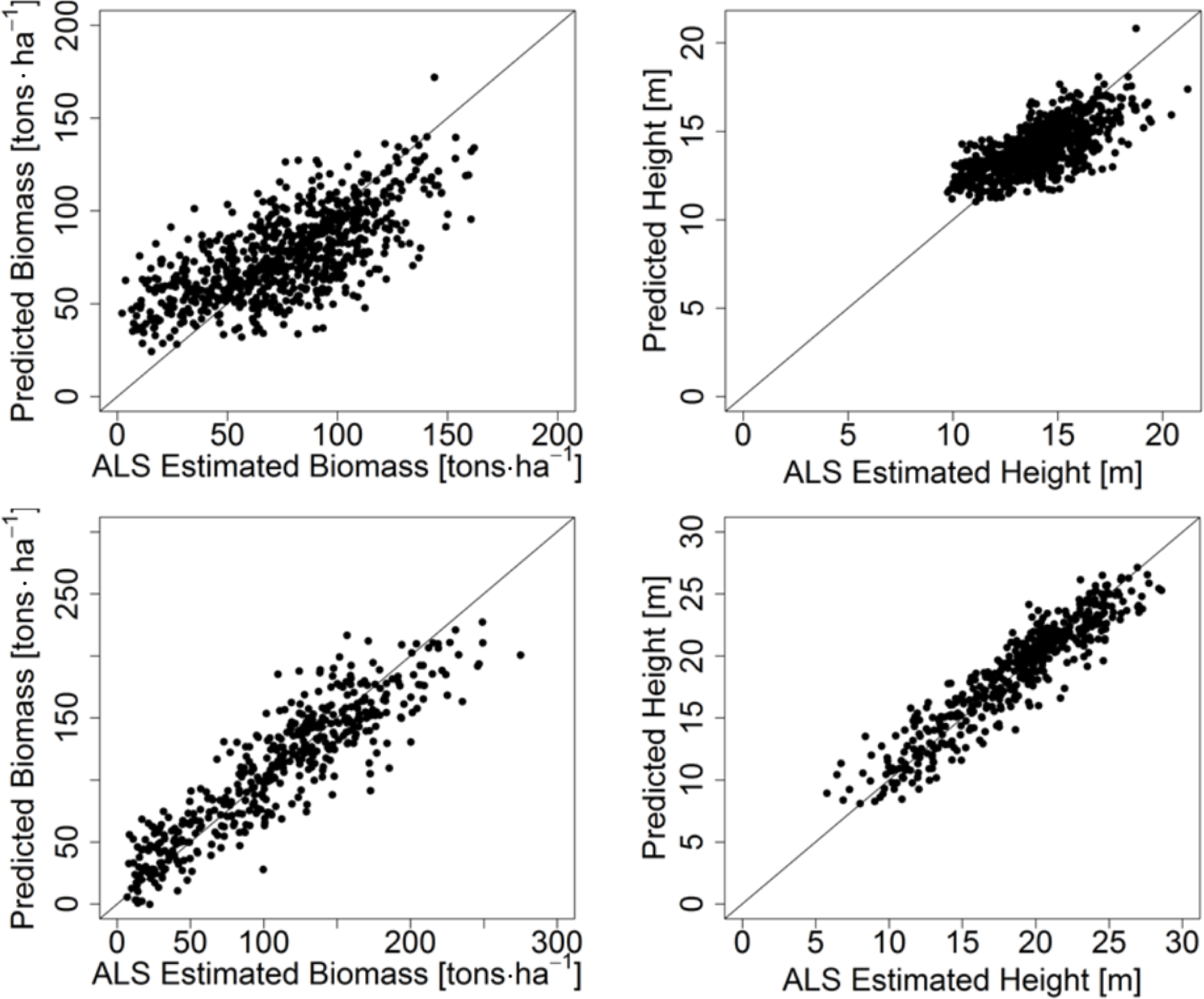
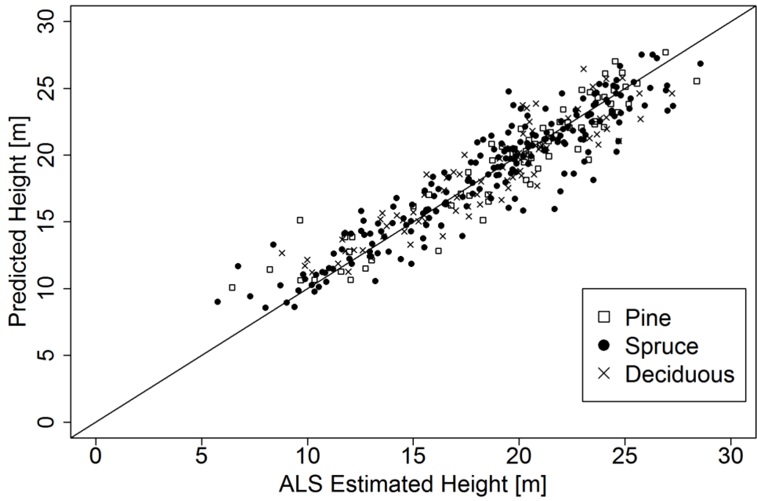
With regards to the H estimations, the adjusted R2 was 0.87 and 9.4% in terms of relative RMSE at Remningstorp. The scatter plots showed a relatively large distribution for the regression functions for Krycklan (
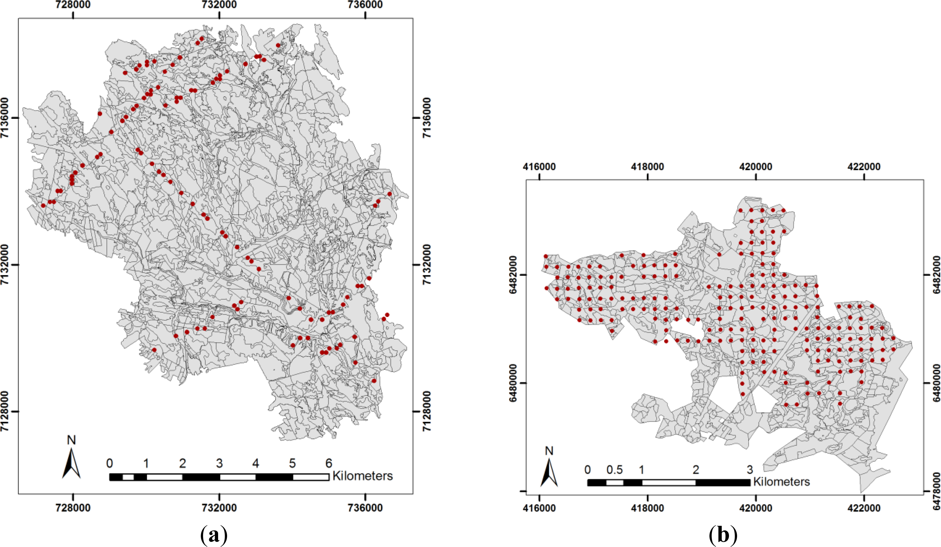
Figure 5, top right), which has a smaller range of available biomasses and tree heights. This suggests a lower height sensitivity at Krycklan, which is likely due to the combination of lower quality radar data and less accurate reference data than for Remningstorp. At Krycklan, 110 field plots were extrapolated to cover 6780 ha compared to Remningstorp where 212 field plots were extrapolated to 1200 ha. As all the radar data from Remningstorp were acquired in HS mode, these present a much higher detail quality (Figure 3) than for Krycklan where the radar images were acquired in SL or SM mode. The scatter plot (Figure 5, bottom) also reflects this, showing a more linear trend with low spread, leading to the significant difference in adjusted R2.
From manual inspection, it was found that many of the stands with largest estimation errors of AGB and H were young forests with low forest heights or sparse forest. This is rather often the case in Krycklan and less frequent in Remningstorp. These forests often show a different proportional relationship between AGB and H compared to more mature forests. The young and sparse forest stands were not easily eliminated, as they both contained low and high AGB, and sometimes low and sometimes relatively high heights, without possessing high AGB. The entire range of H is limited especially in Krycklan, causing strong leverage effects for the remaining stands and not resulting in better overall models. It is fair to assume that the usually thinner, still tall, stems in younger forests get penetrated to a higher degree than mature forests, while the manual field measures still reach high H. In summary, AGB and H for young forest stands are more difficult to estimate accurately with X-band radar.
The effects of the incidence angles of the radar images could not be examined due to a limited number of SAR images, however the effects of the intersection angles were shown to be ambiguous. Previous studies [1719] have concluded that the optimal intersection angles should be about 8–20°. The data in this study can generally verify this as all the successful image matchings in the study used image pairs with intersection angles between 6.9° and 15.3°. However, the conclusion that a larger intersection angle within this span would result in a better height precision can only be confirmed for certain conditions. Matching results from the Krycklan test site showed better results for 6.9° intersection angle than 8.4°, but that the 15.3° image pair showed the best results. The reason for this is not entirely clear, but it is likely that the lower radar image quality of the image KR1 caused the resulting poorer results. In addition, the temporal difference between the SAR images was larger with KR1. These results can be seen to validate the claim by [17]; “For example, larger ray intersection angles and higher spatial resolution do not translate into higher accuracy. In various experiments, accuracy trends even reverse, especially for rough topography”. Krycklan is more strongly influenced by its hillier topography than Remningstorp and fits well into this statement.
It was shown in [21,35] that image triplets, i.e., combining three images with different incidence angles, can make use of both the higher similarities between images with small intersection angles and the increased parallaxes precisions to create more accurate DSMs. This could not be verified in this study, however, we see no reason to doubt that this is the case, assuming all the images included in the triplet bear the same quality.
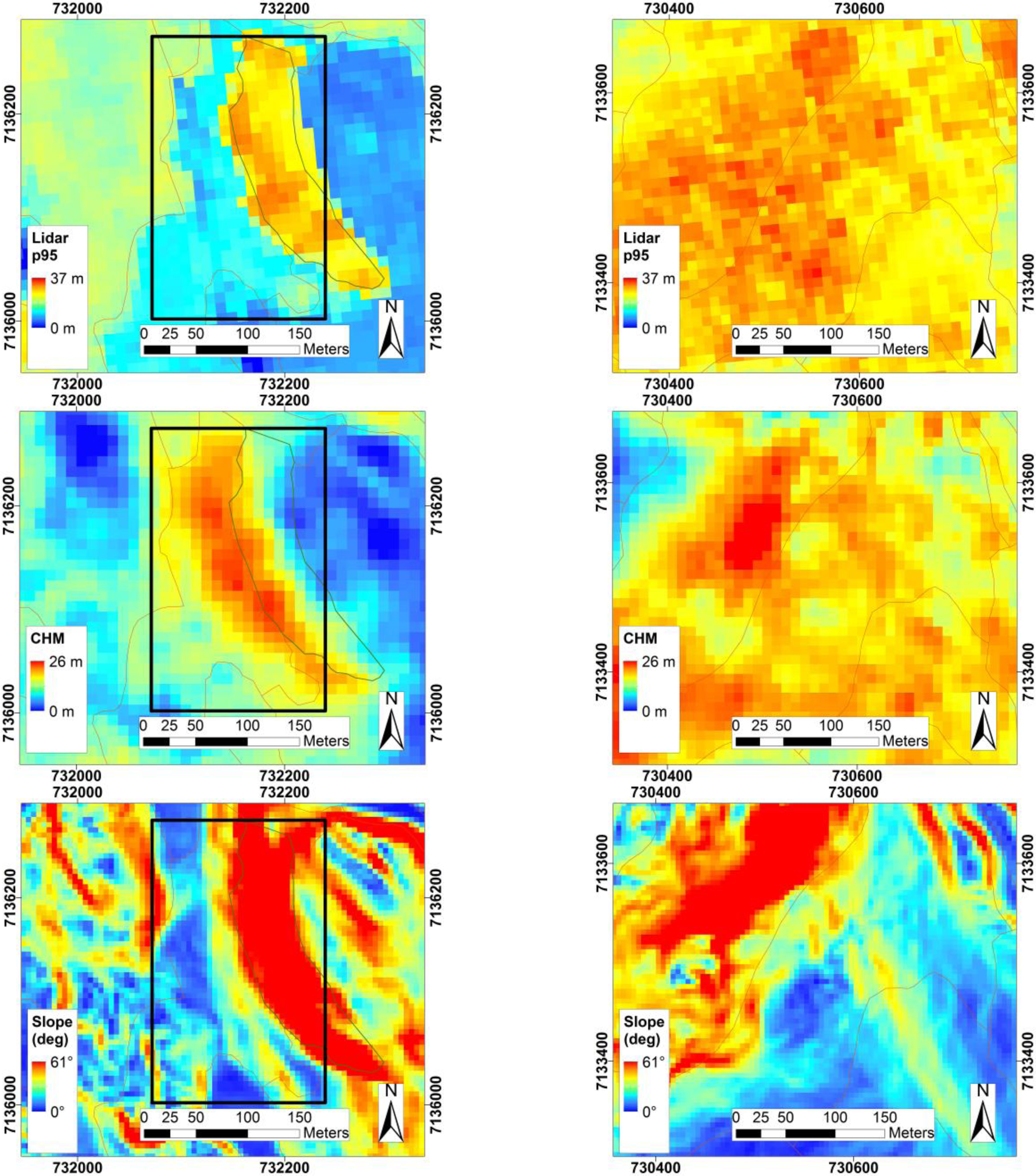
A crucial part of the image matching involved selecting appropriate search window sizes and this clearly depended on the topography. It was noted that the Krycklan test site required a search windows on the order of 10 times larger than for Remningstorp, which was entirely a consequence of the hillier topography. This unfortunately also leads to more false matches, especially in highly heterogeneous terrain. This became clear when a few stands lying in dehydrated river beds were investigated. The ground elevation went down while the DSM remained constant, resulting in unusually high heights in the CHM (Figures 5 and 7).
All radar images used for Krycklan were taken during rainy days with some precipitation and only one acquisition from Remningstorp was affected by precipitation. All DSMs derived from rain influenced images show a lower correlation to the reference data, however due to the many factors that can also potentially affect the results (such as different resolutions, reference data and temporal differences), from the data presented here there is not a strong enough base to conclude that rain has a direct effect on the results. This is however an area that should be investigated further in future studies. All our data sets were acquired in the late summer to late fall (in Krycklan the fall has often already passed in mid-October) and nothing can therefore be concluded about the possible effects of winter images with frozen conditions. This study does however contribute to the general knowledge base by extending the different seasons thus far investigated within radargrammetry [23,24] with another season.
The very comprehensive study presented in [23] was essentially accomplished in pure deciduous forest conditions and the present study together with [24] complements [23] by covering mostly boreal forests made up of essentially pine and spruce stands. The first extended analysis showed that it was not necessary to develop species independent models as long as leaf-on conditions were supplied. Pine, spruce and deciduous (mainly birch) stands seemed to interact in a similar manner to the X-band radar, at least with radargrammetry in boreal forests. At the Krycklan site, the images were acquired during leaf-off conditions and, here, it is also clear that the regression models for deciduous stands did not hold, whereas pine and spruce still responded in line with the overall test site results and also more in line with those from the Remningstorp test site.
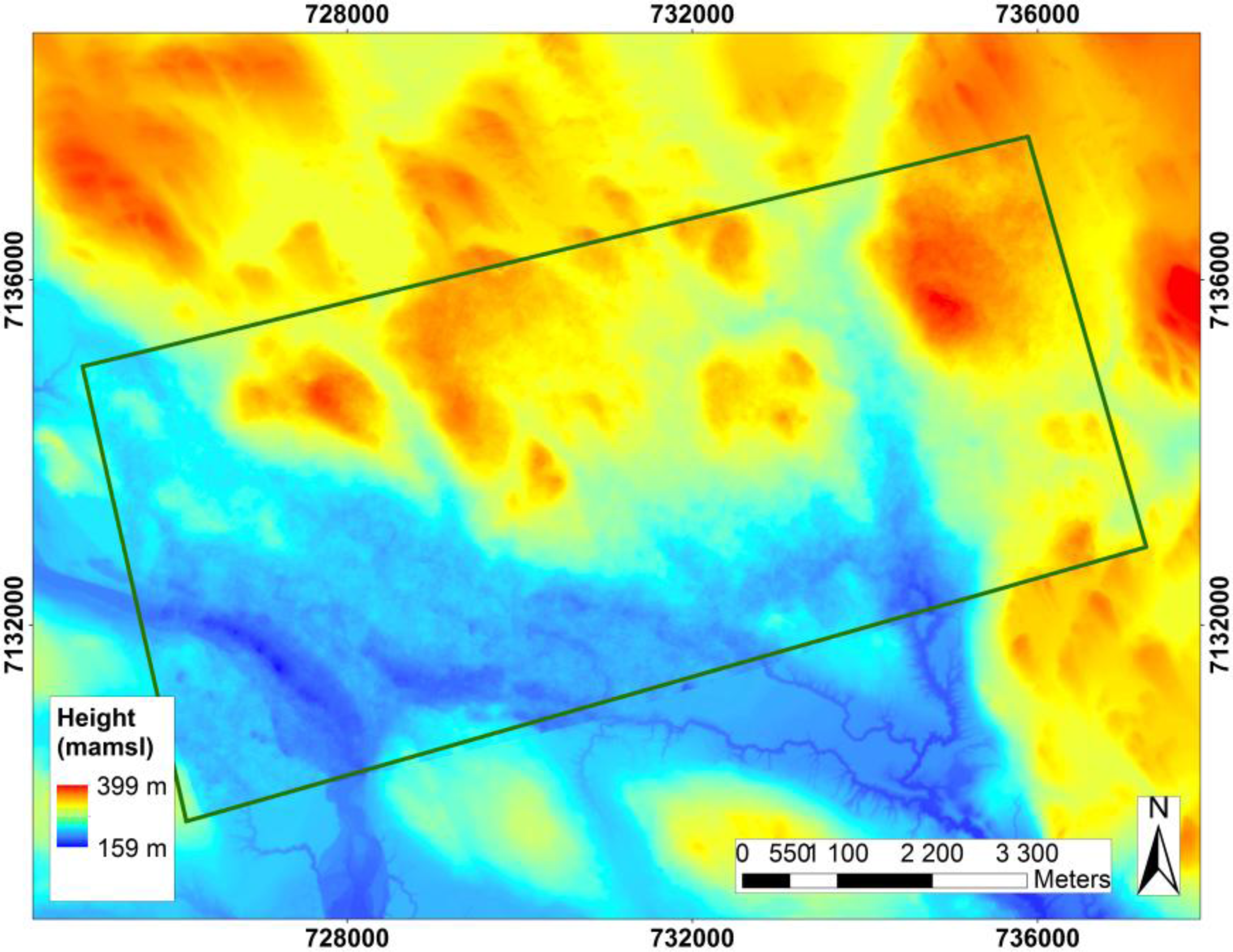
It can be noted that the topography (in addition to the intersection angle and resolution) factor most strongly influencing whether or not a usable full coverage DSM is obtained. This is in agreement with [40] where the authors showed that the principal parameters influencing the accuracy of the DTM are the type of the relief and its slope. In the second extended study presented here this topography problem was rudimentarily tackled by dividing the forest stands into slope classes, where the mean slope of the stand determined its assignment to one of the classes 0–2°, 2–4°, 4–6°, 6–8°, or >8°. The regression models were also complemented with the slope, aspect and the product of these two variables as additional independent variables explaining the AGB and H. It was found that an overall trend could be seen with an increase in the relative RMSE in connection with an increase of the mean slope. It could also be discerned that the product slope×aspect became significant for all regression models >4° and that topography had an influence in sparse conifer forests (as was the case at Krycklan) already from small mean slope values. In practice, these stands often included stronger slopes above 10° even if the average slope finished up in a lower defined slope class.
From visual inspection (Figure 7), it was noted that the results from the slope class models did not give a complete or even fair understanding of the problem. Krycklan with its hilly topography contains many regions with slopes up to 61°. The DSM outcome was heavy influenced by shadowing, foreshortening and layover effects that shifted the heights into completely different stands than where the actual slope was located. In comparison, Remningstorp with its moderate topography was far simpler to process and showed lower residuals. This implied that the shape of the stand appeared to have a significant effect on the outcome. When narrow stands (only a few 10 m wide) were located next to strong slopes, the slope effects spilled over on to the neighboring stands often resulting in a shift in their actual locations (Figure 7). When the stands had a more compact shape (like a circle or a square), the mean height to a greater degree got smeared out by the entire stand mean pixels.
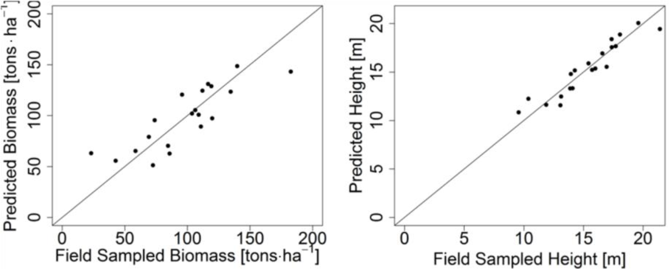
In the third extended study, yet another approach was tried in order to address this topography related problem and eliminate ambiguities related to slopes. Independently inventoried reference field data from the BioSAR 2008 campaign [29] was used for estimating AGB and H at Krycklan. Out of the entire set of stands previously used at Krycklan, 20 stands had intersecting TerraSAR-X data and densely sampled field data. These stands were located in flatter terrain with a lower level of surrounding slopes and if the stands did contain slopes they did not have as large standard deviations of the slopes, meaning that the shifting effects became much smaller. The AGB could now be estimated with an adjusted R2 that was 0.66 and for H it was 0.87 (compared to 0.48 and 0.49 respectively with regards to the entire Krycklan test site). The relative RMSE was also reduced to 23.5% and 7.7% (Table 11) for AGB and H, respectively, compared to the entire test site values of 31.6% and 10.3% (Tables 4 and 5). With such a small data set, despite a higher quality, the modeling resulted in a certain degree of overfitting with q values equal to 1.20. Nonetheless, cautious conclusions indicate that by using the stands located on flatter terrain at Krycklan, results on the same order as Remningstorp can be attained. This demonstrates the robustness of radargrammetry and would also further validate its use for forestry applications with the careful consideration of the possible topography effects.

6. Conclusions

By using TerraSAR-X data acquired from different view angles, DSMs could be created using radargrammetry for the two test sites; Krycklan and Remningstorp, located in northern and southern Sweden, respectively. Highly accurate DTMs from ALS were available for the test sites and the elevation differences were calculated to derive CHMs for both test sites. Reference data consisting of field measured plots from the same years as the radar and ALS data were acquired, were extrapolated by ALS measured height percentiles and density measures to create reference rasters describing AGB and H. Different CHM metrics, where the mean height was most important, were used to model the AGB and H using multiple linear regression.
This study has shown that radargrammetry is a powerful technique which can be used with high resolution X-band SAR data for estimating AGB and H. Images with intersection angles in the range of 8–16° have shown to deliver accurate DSMs. When these can be combined with accurate ALS derived DTMs, AGB on the order of 25%–30% relative RMSE and H on the order of 10% at stand level are realistic. Young forests can be difficult to estimate correctly and potentially should be assigned to their own species class. During leaf-on conditions, different tree species in the boreal forests interact in a similar fashion to the X-band radar waves. Seasonal effects, as well as weather effects, have not been evaluated and should be subject to future research. Regions with more varied topography or sudden changes in DTMs are likely to lead to large local deviations and might have to be aggregated in order to give more for accurate estimations. Topographic slope corrections that can be integrated in the radargrammetric processing chain are important if for radargrammetry is to become a potential tool in forestry. The slope has a significant impact on the estimations already at average slopes >4° at stand level.
From the results, radargrammetry appears to be a potentially promising remote sensing technique for future forest applications.

Acknowledgments

The TerraSAR-X images were acquired through the German Aerospace Center (DLR) TSX-Archive-2012 project (LAN-1895). The processing of DSMs was undertaken with the software RSG from Joanneum Research, Graz, Austria. We would like to especially acknowledge Johann Raggam and his colleagues at Joanneum Research for valuable technical support. This study was financed by the Swedish National Space Board through the project “Retrieval of forest biomass and biomass change with spaceborne SAR”, contract No. 174/12 and by the Hildur & Sven Wingqvist foundation. It has also received funding from the European Community’s Seventh Framework Programme (FP7/2007–2013) under grant agreement No. 606971, the Advanced_SAR project. We would also like to thank the Swedish Meteorological and Hydrological Institute (SMHI) for providing weather data according to the regulations for “Evaluation of forestry applications using new SAR and optical images. Cooperation with SLU, Umeå”. Finally we would like to thank Neil Cory for the proof reading and all the reviewers for constructive comments.

Author Contributions

The study was prepared and accomplished by Henrik Persson, who also prepared the manuscript. Johan Fransson helped with discussions and manuscript revisions.

Conflicts of Interest

The authors declare no conflict of interest.

References

  1. GOFC-GOLD, A Sourcebook of Methods and Procedures for Monitoring and Reporting Anthropogenic Greenhouse Gas Emissions and Removals Associated with Deforestation, Gains and Losses of Carbon Stocks in Forests Remaining Forests, and Forestation; GOFC-GOLD Land Cover Project Office, Wageningen University: Wageningen, The Netherlands, 2012; p. 126.
  2. Rosenqvist, Å.; Milne, A.; Lucas, R.; Imhoff, M.; Dobson, C. A review of remote sensing technology in support of the Kyoto Protocol. Environ. Sci. Policy 2003, 6, 441–455. [Google Scholar]
  3. Patenaude, G.; Milne, R.; Dawson, T.P. Synthesis of remote sensing approaches for forest carbon estimation: Reporting to the Kyoto Protocol. Environ. Sci. Policy 2005, 8, 161–178. [Google Scholar]
  4. Patenaude, G.; Hill, R.; Milne, R.; Gaveau, D.L.A.; Briggs, B.B.J.; Dawson, T.P. Quantifying forest above ground carbon content using LiDAR remote sensing. Remote Sens. Environ 2004, 93, 368–380. [Google Scholar]
  5. Swedish National Forest Inventory, Skogsdata 2013; Swedish National Forest Inventory: Umeå, Sweden, 2013; p. 162.
  6. Hyyppä, J.; Hyyppä, H.; Leckie, D.; Gougeon, F.; Yu, X.; Maltamo, M. Review of methods of small-footprint airborne laser scanning for extracting forest inventory data in boreal forests. Int. J. Remote Sens 2008, 29, 1339–1366. [Google Scholar]
  7. Reutebuch, S.E.; Mcgaughey, R.J.; Andersen, H.; Carson, W.W. Accuracy of a high-resolution lidar terrain model under a conifer forest canopy. Can. J. Remote Sens 2003, 29, 527–535. [Google Scholar]
  8. Nilsson, M. Estimation of tree heights and stand volume using an airborne lidar system. Remote Sens. Environ 1996, 56, 1–7. [Google Scholar]
  9. St-Onge, B.; Hu, Y.; Vega, C. Mapping the height and above-ground biomass of a mixed forest using lidar and stereo Ikonos images. Int. J. Remote Sens 2008, 29, 1277–1294. [Google Scholar]
  10. Koch, B. Status and future of laser scanning, synthetic aperture radar and hyperspectral remote sensing data for forest biomass assessment. ISPRS J. Photogramm. Remote Sens 2010, 65, 581–590. [Google Scholar]
  11. La Prade, G. An analytical and experimental study of stereo for radar. Photogramm. Eng. Remote Sens 1963, 29, 294–300. [Google Scholar]
  12. Bresnahan, P.C. Geolocation Accuracy Re-Evaluation of Cosmo-Skymed Spotlight and Stripmap Imaging Mode Products; National Geospatial-Intelligence Agency: Boulder, CO, USA, 2011. [Google Scholar]
  13. Fritz, T.; Breit, H.; Eineder, M. TerraSAR-X Products—Tips and tricks. Proceedings of the 3rd TerraSAR-X Workshop, Oberpfaffenhofen, Germany, 25–26 November 2008; p. 61.
  14. Schubert, A.; Jehle, M.; Small, D.; Meier, E. Geometric Validation of TerraSAR-X High-Resolution Products. Proceedings of the 3rd TerraSAR-X Workshop, Oberpfaffenhofen, Germany, 25–26 November 2008; p. 6.
  15. Ager, T.P.; Bresnahan, P.C. Geometric Precision in Space Radar Imaging: Results from TerraSAR-X. Proceedings of the ASPRS 2009 Annual Conference, Baltimore, MD, USA, 9–13 March 2009; p. 8.
  16. Raggam, H.; Gutjahr, K.; Perko, R.; Schardt, M. Assessment of the stereo-radargrammetric mapping potential of TerraSAR-X multibeam spotlight data. IEEE Trans. Geosci. Remote Sens 2010, 48, 971–977. [Google Scholar]
  17. Toutin, T.; Gray, L. State-of-the-art of elevation extraction from satellite SAR data. ISPRS J. Photogramm. Remote Sens 2000, 55, 13–33. [Google Scholar]
  18. Kaupp, V.H.; Bridges, L.C.; Pisaruck, M.A.; Macdonald, H.C.; Waite, W.P. Simulation of spaceborne stereo radar imagery: Experimental results. IEEE Trans. Geosci. Remote Sens 1983, 21, 400–405. [Google Scholar]
  19. Mercer, J.B. SAR Technologies for Topographic Mapping. In Photogrammetric Week “95”; Fritsch, D., Hobbie, D., Eds.; Wichmann Verlag: Heidelberg, Germany, 1995; pp. 117–126. [Google Scholar]
  20. Perko, R.; Raggam, H.; Gutjahr, K.; Schardt, M. The Capabilities of TerraSAR-X Imagery for Retrieval of Forest Parameters. Proceedings of the ISPRC TC VII Symposium, Vienna, Austria, 5–7 July 2010; pp. 452–456.
  21. Perko, R.; Raggam, H.; Gutjahr, K.; Schardt, M. Deriving Forest Canopy Height Models Using Multi-Beam TerraSAR-X Imagery. Proceedings of the 8th European Conference on Synthetic Aperture Radar (EUSAR), Aachen, Germany, 7–10 June 2010; pp. 568–571.
  22. Perko, R.; Raggam, H.; Gutjahr, K.; Schardt, M. Analysis of 3D Forest Canopy Height Models Resulting from Stereo-Radargrammetric Processing of TerraSAR-X Images. In Proceedings of the 30th EARSeL Symposium, Remote Sensing for Science, Education, and Natural and Cultural Heritage. Paris, France, 31 May–3 June 2010; p. 8.
  23. Perko, R.; Raggam, H.; Deutscher, J.; Gutjahr, K.; Schardt, M. Forest assessment using high resolution SAR data in X-band. Remote Sens 2011, 3, 792–815. [Google Scholar]
  24. Karjalainen, M.; Kankare, V.; Vastaranta, M.; Holopainen, M.; Hyyppä, J. Prediction of plot-level forest variables using TerraSAR-X stereo SAR data. Remote Sens. Environ 2012, 117, 338–347. [Google Scholar]
  25. Vastaranta, M.; Holopainen, M.; Karjalainen, M. TerraSAR-X stereo radargrammetry and airborne scanning LiDAR height metrics in imputation of forest aboveground biomass and stem volume. IEEE Trans. Geosci. Remote Sens 2014, 52, 1197–1204. [Google Scholar]
  26. Horn, B.K.P. Hill shading and the reflectance map. Proc. IEEE 1981, 69, 14–47. [Google Scholar]
  27. Lindberg, E. Estimation of Canopy Structure and Individual Trees from Laser Scanning Data; Swedish University of Agricultural Sciences: Uppsala, Swedish, 2012; p. 78. [Google Scholar]
  28. Marklund, L.G. Biomass Functions for Pine, Spruce and Birch in Sweden; Swedish University of Agricultural Sciences, Department of National Forest Inventory: Umeå, Sweden, 1988. [Google Scholar]
  29. Hajnsek, I.; Scheiber, R.; Keller, M.; Horn, R.; Lee, S.; Ulander, L.M.H.; Gustavsson, A.; Sandberg, G.; Toan, T.L.; Tebaldini, S.; Guarnieri, A.M.; Rocca, F. BIOSAR 2008 Technical Assistance for the Development of Airborne SAR and Geophysical Measurements during the BioSAR 2008 Experiment; ESA Contract No. 22052/08/NL/CT; European Space Agency: Noordwijk, The Netherlands, 2009. [Google Scholar]
  30. Ulander, L.M.H.; Gustavsson, A.; Flood, B.; Murdin, D.; Dubois-Fernandez, P.; Dupuis, X.; Sandberg, G.; Soja, M.J.; Eriksson, L.E.B.; Fransson, J.E.S.; et al. BioSAR 2010. Technical Assistance for the Development of Airborne SAR and Geophysical Measurements during the BioSAR 2010 Experiment: Final Report; ESA Contract No. 4000102285/10/NL/JA/ef; European Space Agency: Noordwijk, The Netherlands, 2010. [Google Scholar]
  31. Lundgren, J.; Juni, O. Noggrannhetskontroll av Laserdata för ny Nationell Höjdmodell; Högskolan i Gävle: Gävle, Sweden, 2010. [Google Scholar]
  32. Ulander, L.M.H.; Gustavsson, A.; Dubois-Fernandez, P.; Dupuis, X.; Fransson, J.E.S.; Holmgren, J.; Wallerman, J.; Eriksson, L.; Sandberg, G.; Soja, M.; et al. BIOSAR 2010—A SAR Campaign in Support to the BIOMASS Mission. Proceedings of IGARSS 2011 IEEE International Symposium on Geoscience and Remote Sensing, Vancouver, Canada, 24–29 July, 2011; pp. 1528–1531.
  33. Fritz, T.; Eineder, M. TerraSAR-X Ground Segment Basic Product Specification Document; German Aerospace Center (DLR): Oberpfaffenhofen, Germany, 2008; p. 103. [Google Scholar]
  34. Joanneum Research Remote Sensing Graz. Available online: http://dib.joanneum.at/rsg/ (accessed on 8 January 2013).
  35. Raggam, H. Surface mapping using image triplets: Case studies and benefit assessment in comparison to stereo image processing. Photogramm. Eng. Remote Sens 2006, 72, 551–563. [Google Scholar]
  36. Paar, G.; Pölzleitner, W. Robust Disparity Estimation in Terrain Modeling for Spacecraft Navigation. Proceedings of the 11th IAPR International Conference on Pattern Recognition, The Hague, The Netherlands, 30 August–3 September 1992; pp. 738–741.
  37. Eldhuset, K.; Weydahl, D.J. Geolocation and stereo height estimation using TerraSAR-X spotlight image data. IEEE Trans. Geosci. Remote Sens 2011, 49, 3574–3581. [Google Scholar]
  38. Weisberg, S. Applied Linear Regression, 2nd ed; John Wiley & Sons: New York, NY, USA, 1985. [Google Scholar]
  39. Lehtonen, A.; Mäkipää, R.; Heikkinen, J.; Sievänen, R.; Liski, J. Biomass expansion factors (BEFs) for Scots pine, Norway spruce and birch according to stand age for boreal forests. For. Ecol. Manage 2004, 188, 211–224. [Google Scholar]
  40. Toutin, T. Evaluation of radargrammetric DEM from RADARSAT images in high relief areas. IEEE Trans. Geosci. Remote Sens 2000, 38, 782–789. [Google Scholar]
Figure 1. The two test sites Krycklan and Remningstorp, located in northern (64°N) and southern (58°N) Sweden, respectively.
Remotesensing 06 02084f1
Figure 2. The forest stand delineation and field plot distribution of the two test sites. (a) Krycklan; (b) Remningstorp.
Remotesensing 06 02084f2
Figure 3. Illustration of the information content from a subset of an ortho-rectified GammaMAP-filtered TerraSAR-X image acquired 17 October 2008, over Krycklan (Top) and 2 September 2010, over Remningstorp (Bottom).
Remotesensing 06 02084f3
Figure 4. The Krycklan test site with an ALS DTM overlaid by a DSM (delineated in green) derived from TerraSAR-X SL data.
Remotesensing 06 02084f4
Figure 5. Scatter plots of AGB (Left) and H (Right) estimations for stands at the Krycklan (Top) and Remningstorp (Bottom) test sites.
Remotesensing 06 02084f5
Figure 6. Scatter plot of tree species-specific H estimations at Remningstorp.
Remotesensing 06 02084f6
Figure 7. Topography affected stands at Krycklan. In the foreslope (Left), the central stand with low heights gets high heights shifted into its stand caused by the slope located in the stand to the right (61°). In the backslope (Right) this effect is negligible. Top: ALS percentile 95 height raster. Middle: TerraSAR-X derived height raster. Bottom: Slope raster derived from ALS data. The TerraSAR-X images are acquired from the left side in these images.
Remotesensing 06 02084f7
Figure 8. Scatter plots for the 20 flatter stands at Krycklan using field reference data from the BioSAR 2008 campaign, AGB (Left) and H (Right).
Remotesensing 06 02084f8
Table 1. Properties for the derived reference rasters with AGB in tons·ha−1 and H in m.
Test SiteRMSE% AGBRMSE% HAGB MinAGB MeanAGB MaxAGB SdH MinH MeanH MaxH Sd
Krycklan19.96.7277162349.714.121.12.1
Remningstorp12.711.27110275584.718.328.64.9
Table 2. The list of TerraSAR-X satellite images used for the Krycklan (KR) test site.
Image# KRAcquisition DatePolarizationOrbit/Antenna DirectionModeInc. Angle (°)Time (UTC)Resolution rg/az (m)GSD (m)Precipitation (mm)
111 October 2008HH/HVAsc/RightSM40.716:121.18/6.062.753.5
216 October 2008HHAsc/RightSL47.616:211.18/1.380.509.5
317 October 2008HH/VVAsc/RightSL32.316:041.18/3.521.5012.3
Table 3. The list of TerraSAR-X satellite images used for the Remningstorp (RE) test site.
Image# REAcquisition DatePolarizationOrbit/Antenna DirectionModeInc. Angle (°)Time (UTC)Resolution rg/az (m)GSD rg/az (m)Precipitation (mm)
122 August 2010HHAsc/RightHS40.516:451.18/1.100.91/0.860
227 August 2010HHAsc/RightHS49.616:541.18/1.100.91/0.875.5
32 September 2010HH/HHAsc/RightHS40.516:451.18/1.100.91/0.860
47 September 2010HH/HHAsc/RightHS49.616:541.18/1.100.91/0.870
Table 4. The results for estimating AGB at both test sites.
Image#Test SiteIntersection Angle (°)R2adjRMSE (tons·ha−1)RMSE (%)qNo. of Stands
KR1-2Krycklan6.90.2828.536.91.00752
KR1-3Krycklan8.40.2030.139.01.00754
KR2-3Krycklan15.30.4824.331.61.00748
KR1-2-3Krycklan6.9, 8.4, 15.30.4724.531.81.00749
RE1-2Remningstorp8.10.7529.026.61.01456
RE3-4Remningstorp8.10.8124.922.91.01453
Table 5. The results for estimating H at both test sites.
Image#Test SiteIntersection Angle (°)R2adjRMSE (m)RMSE (%)qNo. of Stands
KR1-2Krycklan6.90.281.712.21.00749
KR1-3Krycklan8.40.191.813.01.00752
KR2-3Krycklan15.30.491.510.31.01744
KR1-2-3Krycklan6.9, 8.4, 15.30.481.510.51.01746
RE1-2Remningstorp8.10.812.111.41.01452
RE3-4Remningstorp8.10.871.79.41.01452
Table 6. Regression model parameters for AGB (tons·ha−1) and H (m) described for Equation (5) at Krycklan at stand level.
EstimatorImage#R2adjRMSERMSE (%)αβ1β2β3β4β5qNo. of Stands
AGBKR1-2-30.4724.531.819.5008.010.101.00749
HKR1-2-30.481.510.510.700.30.81.401.01746
Table 7. Species-specific results of AGB for the image pairs KR2-3 and RE3-4.
Image#Test SiteSpeciesR2adjRMSE (tons·ha−1)RMSE (%)qNo. of Stands
KR2-3KrycklanPine0.5123.233.81.01424
RE3-4RemningstorpPine0.7230.926.81.0371
KR2-3KrycklanSpruce0.5823.522.71.1039
RE3-4RemningstorpSpruce0.8224.521.51.03200
KR2-3KrycklanDeciduous0.1122.832.51.0936
RE3-4RemningstorpDeciduous0.7729.226.11.0582
Table 8. Species-specific results of H for the image pairs KR2-3 and RE3-4.
Image#Test SiteSpeciesR2adjRMSE (m)RMSE (%)qNo. of Stands
KR2-3KrycklanPine0.441.611.51.01422
RE3-4RemningstorpPine0.881.78.81.0470
KR2-3KrycklanSpruce0.451.59.81.0839
RE3-4RemningstorpSpruce0.861.89.91.01199
KR2-3KrycklanDeciduous0.121.29.11.1136
RE3-4RemningstorpDeciduous0.831.89.81.0482
Table 9. Slope class results of AGB at Krycklan.
Image#Test SiteSlope (°)R2adjRMSE (tons·ha−1)RMSE (%)qNo. of Stands
KR2-3Krycklan<20.2830.745.31.0486
KR2-3Krycklan2–40.4923.529.31.03208
KR2-3Krycklan4–60.5624.530.41.02180
KR2-3Krycklan6–80.5625.132.61.03122
KR2-3Krycklan>80.3629.440.81.02154
Table 10. Slope class results of H at Krycklan.
Image#Test SiteSlope (°)R2adjRMSE (m)RMSE (%)qNo. of Stands
KR2-3Krycklan<20.531.39.31.0686
KR2-3Krycklan2–40.431.39.41.02207
KR2-3Krycklan4–60.531.49.91.02178
KR2-3Krycklan6–80.561.511.01.03122
KR2-3Krycklan>80.441.611.81.03152
Table 11. Results for the 20 flatter stands at Krycklan using field reference data from the BioSAR 2008 campaign.
Test SiteModelR2adjRMSE (m)RMSE (%)qNo. of Stands
KrycklanAGB0.6623.323.51.2020
KrycklanH0.871.27.71.2020

