Article

Assessing the Temporal Stability of the Accuracy of a Time Series of Burned Area Products

1
Department of Geology, Geography and Environment, University of Alcalá, C/ Colegios 2, Alcalá de Henares 28801, Spain
2
Department of Forest and Natural Resources Management, College of Environmental Science and Forestry, State University of New York, Syracuse, NY 13210, USA
3
Departamento de Estadística y MGA, ETSI Agrónomos, Universidad Politécnica de Madrid, Ciudad Universitaria, Madrid 28040, Spain
*
Author to whom correspondence should be addressed.
Remote Sens. 2014, 6(3), 2050-2068; https://doi.org/10.3390/rs6032050
Submission received: 22 October 2013 / Revised: 14 February 2014 / Accepted: 27 February 2014 / Published: 6 March 2014
(This article belongs to the Special Issue Quantifying the Environmental Impact of Forest Fires)

Abstract

:
Temporal stability, defined as the change of accuracy through time, is one of the validation aspects required by the Committee on Earth Observation Satellites’ Land Product Validation Subgroup. Temporal stability was evaluated for three burned area products: MCD64, Globcarbon, and fire_cci. Traditional accuracy measures, such as overall accuracy and omission and commission error ratios, were computed from reference data for seven years (2001–2007) in seven study sites, located in Angola, Australia, Brazil, Canada, Colombia, Portugal, and South Africa. These accuracy measures served as the basis for the evaluation of temporal stability of each product. Nonparametric tests were constructed to assess different departures from temporal stability, specifically a monotonic trend in accuracy over time (Wilcoxon test for trend), and differences in median accuracy among years (Friedman test). When applied to the three burned area products, these tests did not detect a statistically significant temporal trend or significant differences among years, thus, based on the small sample size of seven sites, there was insufficient evidence to claim these products had temporal instability. Pairwise Wilcoxon tests comparing yearly accuracies provided a measure of the proportion of year-pairs with significant differences and these proportions of significant pairwise differences were in turn used to compare temporal stability between BA products. The proportion of year-pairs with different accuracy (at the 0.05 significance level) ranged from 0% (MCD64) to 14% (fire_cci), computed from the 21 year-pairs available. In addition to the analysis of the three real burned area products, the analyses were applied to the accuracy measures computed for four hypothetical burned area products to illustrate the properties of the temporal stability analysis for different hypothetical scenarios of change in accuracy over time. The nonparametric tests were generally successful at detecting the different types of temporal instability designed into the hypothetical scenarios. The current work presents for the first time methods to quantify the temporal stability of BA product accuracies and to alert product end-users that statistically significant temporal instabilities exist. These methods represent diagnostic tools that allow product users to recognize the potential confounding effect of temporal instability on analysis of fire trends and allow map producers to identify anomalies in accuracy over time that may lead to insights for improving fire products. Additionally, we suggest temporal instabilities that could hypothetically appear, caused by for example by failures or changes in sensor data or classification algorithms.

1. Introduction

Validation is a critical step of every remote sensing project as it provides a quantitative assessment of the reliability of results and transmits critical information to end users [1]. The Committee on Earth Observing Satellites’ (CEOS) Land Product Validation (LPV) Subgroup defines validation as: “The process of assessing, by independent means, the quality of the data products derived from the system outputs”. When a series of maps is produced over time, temporal stability of accuracy is one of the most important aspects to be evaluated. CEOS-LPV requires an assessment of temporal stability to satisfy the criteria defined in Stage 2 for a product validation process ( http://lpvs.gsfc.nasa.gov).
This research is part of the fire_cci project ( http://www.esa-fire-cci.org), which is tasked with producing globally consistent time series of burned area (BA) data at 300 m to 1000 m spatial resolutions for serving the needs of climate modelers. The fire_cci project is part of the European Space Agency’s Climate Change Initiative (CCI), which aims to generate Essential Climate Variables (ECV), mainly from European space-borne sensors. The program covers 13 ECVs, including atmospheric, marine, and terrestrial variables [2]. As this program is driven by climate modelers, a critical component of the CCI program is validation and uncertainty characterization. A user survey was conducted at the beginning of the fire_cci project to identify the specific needs of validation information [3]. Temporal stability was defined by users as a critical aspect of accuracy assessment, with global agreement and bias of the BA products identified as other accuracy measures of interest.
Several approaches have been used to characterize accuracy of BA products. The most common approach is based on cross tabulating the generated products and reference maps of sampled areas, generating pixel-level error matrices [47]. Other authors have suggested using linear regression analysis, based on the comparison between the proportions of BA detected by the global and by the reference products [6,8,9]. These proportions are computed from an auxiliary grid, with five to 10 times coarser resolution than the target global product. A third common approach is based on landscape pattern analysis. For instance, Chuvieco et al. [5] compared the number of fires estimated by the global and reference products, while Giglio et al. [4] used linear regression to analyze true and estimated fire patch sizes. The choice of the validation methods and objectives should be driven by the final use of the global product. Hence, no single validation approach is universally best. The key is to construct the validation to assess product features relevant to the final product user. The present study followed the cross tabulation approach due to its common use [1,10] and familiarity to a broad scientific community.
Thematic accuracy typically refers to the degree to which the derived image classification (i.e., a burned area map in our case) agrees with reality or conforms to the “ground truth” [11,12]. Temporal stability refers to the change of accuracy through time [13]. If accuracy is changing over time, users will justifiably be concerned that temporal trends observed in the map are confounded by variation in accuracy of the time series of maps. As most BA product validation efforts have been based on just one year of reference data, the temporal dimension of accuracy assessment of a time series of products has not received much attention (see Cohen et al. [14] for one exception).
The purpose of this study was to develop methods to quantify temporal stability. To illustrate the techniques and results, we applied the analyses to three BA products, fire_cci (the product developed in the project that supported this study), MCD64A1, and Globcarbon. The fire_cci BA product [15] was derived from merging the results of three different sensors SPOT-VEGETATION (hereafter referred to as VGT), ERS-ATSR and ENVISAT-AATSR (hereafter, the two latter referred to as ATSR) and ENVISAT-MERIS (hereafter referred to as MERIS). The fire_cci product is offered in monthly composites reporting the day of the year of BA detections at the maximum resolution of the three sensors (1000 m generally and 300 m when MERIS is available). The Globcarbon BA product was produced by the European Space Agency from VGT and ATSR, and it reports the day of the year of BA detections at 1 km pixel size. Globcarbon consists of three separate BA algorithm results [16]. For this study we considered a pixel as burned when at least two of the three Globcarbon algorithms detected it as burned. MCD64A1, the MODIS Collection 5.1 Direct Broadcast Monthly Burned Area product (hereafter referred to as MCD64) has 500 m spatial resolution and also reports the date of BA detections. It was produced from MODIS data on board the Terra and Aqua satellites, and it was based on dynamic thresholds to a vegetation index and a temporal texture, guided by active fire detections [4]. Another well-known and commonly used MODIS BA product (MCD45A1) [17] was not included in the analysis because substantial proportions of area for two of the study sites (Canada and Colombia, see next section) were not mapped by MCD45A1 for several years. Thus we did not have a sufficient temporal record for MCD45A1 to allow an assessment for the same years and sites available for the other three BA products evaluated. The absence of MCD45A1 data for Canada (during the time period studied) was particularly important because Canada was the only study site with presence of Boreal forests, one of the primary biomes affected by fire.

2. Methods

2.1. Study Sites

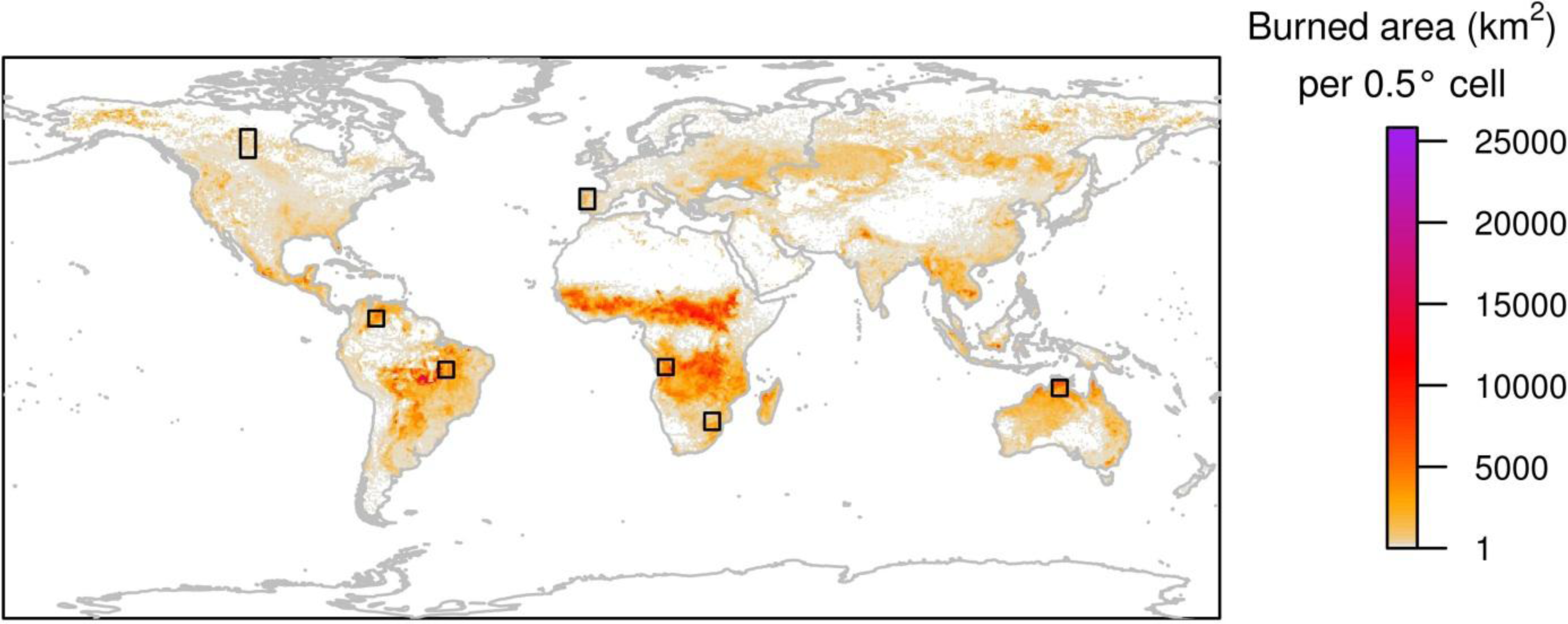
Temporal stability was derived from a set of study sites selected to represent the main ecosystems affected by fire. The reference fire perimeters for each site were derived from multi-temporal analysis of Landsat images, covering seven years (from 2001 to 2007). The seven study sites, each covering an area of 500 km × 500 km were located in Angola, Australia, Brazil, Canada, Colombia, Portugal, and South Africa (Figure 1). Study sites were purposely selected to cover the most problematic areas for burned area discrimination and to represent the major biomes affected by fires (Tropical savannas, Boreal forest, Tropical forest, and Temperate forest). The fire_cci project collected reference data for three other study sites; however these three sites were not included in the analysis as reference data for some years were unavailable. Accuracy is likely to be dependent on the study site (because the sites belong to very different ecosystems). Therefore, we wanted to make sure that data for all study sites were available for each year to ensure a common temporal basis for evaluating all sites. A reference dataset was generated for each study site and year, from 2001 to 2007.
Although these seven sites provide data to illustrate the techniques proposed for assessing temporal stability, it is critical to recognize the limitations of these data when interpreting the results presented in Section 3. To effectively assess temporal stability of fire products, a long time series of reference data would be needed for a large number of sample sites. The time and cost to obtain such reference data are substantial. In this article, we can take advantage of an existing dataset, albeit one with a small sample size, to provide examples of what the analysis of temporal stability entails. A small sample size will likely yield low statistical power to detect departures from temporal stability, so for our illustrative example analysis, it should not be surprising if the statistical tests result in insufficient evidence to reject a null hypothesis that temporal stability is present. Moreover, the seven sample sites were selected specifically to span a broad geographic range, so the accuracy measures estimated from such a small sample will likely have high variance further reducing the power of the tests. A preferred scenario envisioned for an effective assessment of temporal stability would be to have an equal probability sample of 25–30 sites selected from each of six to eight geographic regions (e.g., biomes), and to obtain an annual time series of reference data for each site from which the accuracy measures would be derived. The temporal stability analyses we describe could then be applied to the sample data from each biome. We emphasize that the results and conclusions based on the seven sample sites should be considered as an illustrative, not definitive assessment of temporal stability of the three real fire products.

2.2. Reference Data

Fire reference perimeters for each site and year were produced for the period 2001 to 2007. For each year, two multi-temporal pairs of Landsat TM/ETM+ images (covering around 34,000 km2) were downloaded from the Earth Resources Observation Systems (EROS) Data Center (EDC) of the USGS ( http://glovis.usgs.gov). We selected images that were cloud-free and without the Scan Line Corrector (SLC) failure whenever possible. The dates of image pairs were chosen to be close enough to be sure that the BA signal of fires occurring in between the two dates was still clear in the second date. We tried to select images fewer than 32 days apart for Tropical regions, where the burned signal lasts for only a short time, as fires tend to have low severity and vegetation regenerates quickly. For ecosystems where the burned signal persists longer, such as Temperate and Boreal forest, images could be separated by up to 96 days in some years. A total of 98 Landsat scenes were processed to generate the validation dataset. Burned area perimeters were derived from a semi-automatic algorithm developed by Bastarrika et al. [19]. Outputs of this algorithm were verified visually by one interpreter and reviewed by another. GOFC-GOLD regional experts were contacted to clarify problematic regions where ecological processes producing spectral responses similar to burned area could occur (e.g., vegetation phenology, harvesting or cutting trees). These reference fires were delineated following a standard protocol defined for the fire_cci project [20] (available online at http://www.esa-fire-cci.org/webfm_send/241) and based on the CEOS-LPV guidelines [21]. Unobserved areas due to clouds or sensor problems in the Landsat images were masked out and removed from further analysis. Similarly, only the central parts of the images were considered for ETM images affected by the SLC failure.
BA products included in this study consisted of monthly files with pixel values referring to the burning date (Julian day, 1–365). Burned pixels between the reference image acquisition dates were coded as “burned”. The rest of the area was coded as “unburned” or “no data”, the latter applied to pixels obscured by clouds, with corrupted data, or missing values.

2.3. Accuracy Measurements

The error matrix summarizes two categorical classifications of a common set of sample locations (Table 1). As Landsat-TM/ETM+ images have a much higher spatial resolution (30 m) than the global BA products (500–1000 m), the comparison between the global product and reference data was based on the proportion of each BA product pixel classified as burned in the reference (Landsat) pixels. Therefore, we compiled the error matrix, based on the partial agreement between the product and reference pixels. The error matrix for each Landsat scene and year was obtained by summing the agreement and disagreement proportions of each pixel. For example, a pixel classified as burned for the BA product that had 80% of reference burned pixels would have a proportion of 0.8 as true burned (i.e., p11,u = 0.8 for pixel u) and 0.2 as commission error (p12,u =0.2), but this pixel would have neither omission errors (p21,u = 0) nor true unburned area (p22,u =0). Conversely, a pixel classified as unburned that had 10% of reference pixels detected as burned would have a proportion of 0.9 as true unburned (p22,u =0.9), p21,u =0.1 as omission error, and neither commission error (p12,u =0) nor true burned area (p11,u =0). The error matrix for each study site and year was computed from the sum of the single pixel error matrices:
p ij , ss = u s s p ij , u N ss
where the summation is over all Nss BA product pixels u with available reference data at study site ss. Detailed methods of this process can be found in Binaghi et al. [22], and for stratified samples in Stehman et al. [23].
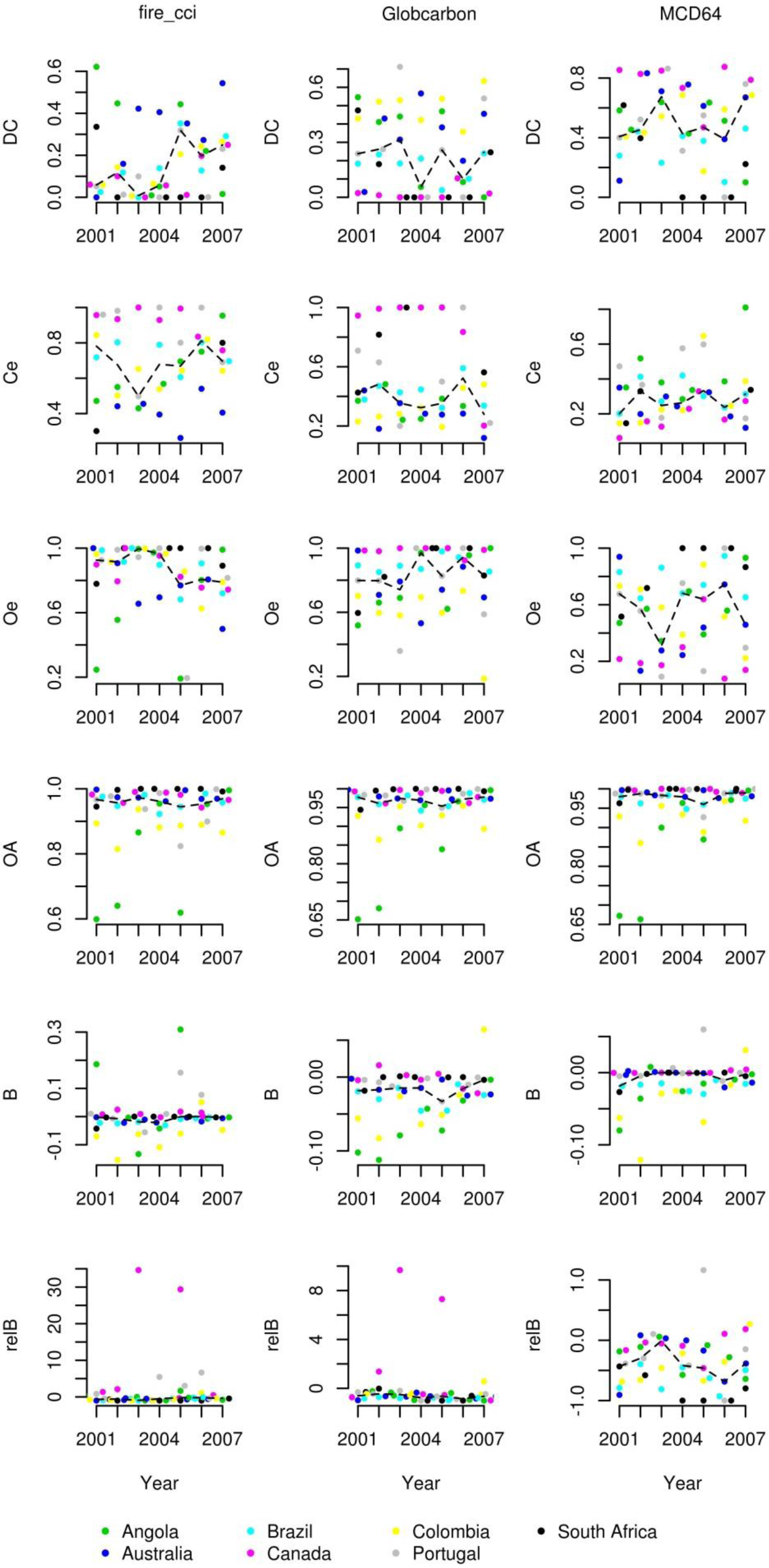
Numerous accuracy measures may be derived from the error matrix. Three measures broadly used and generally accepted in the BA validation literature [57] are overall accuracy:
O A = p 11 + p 22
the commission error ratio:
C e = p 12 / p 1 +
and omission error ratio:
O e = p 21 / p + 1
the two latter referring to the “burned” category. For most users, the accuracy of the “burned” category is much more relevant than the accuracy of unburned areas, as it is more closely related to the impacts of biomass burning on vegetation and atmospheric chemistry. For this reason, measures that focus on the “burned” category are recommended in BA product validation.
OA depends on category-map prevalence [
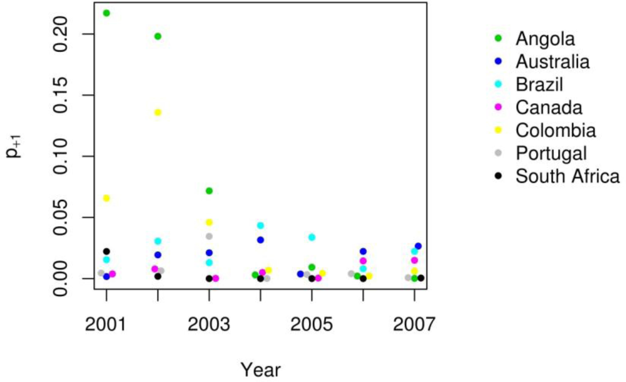
24] so in areas with low fire occurrence, OA may be very stable through time because most of the area will be correctly classified as unburned. For this reason, OA is not expected to be sufficiently sensitive to evaluate temporal stability of a product, as it has a strong dependence on the proportion of burned area (p+1). Ce and Oe are anticipated to be more sensitive measures to changes in accuracy over time.
We also included a measure that combines information related to user’s and producer’s accuracy of BA. Such an aggregate measure of accuracy may be useful in applications in which the user does not have a preference for minimizing either Oe or Ce. The aggregate measure used is the Dice coefficient [2527] defined as:
D C = 2 p 11 2 p 11 + p 12 + p 21
Given that one classifier (product or reference data in our case) identifies a burned pixel, DC is the conditional probability that the other classifier will also identify it as burned [26].
Bias has rarely been considered in BA validation even though it is relevant for climate modelers (e.g., of atmospheric emissions) who are interested in BA products with small over- or under-estimation of the proportion of BA [3]. Bias expressed in terms of proportion of BA is defined as:
B = p 1 + p + 1 = p 12 p 21
The bias can also be scaled relative to the reference BA:
relB = p 1 + p + 1 p + 1 = p 12 p 21 p + 1
B and relB values above zero indicate that the product overestimates the extent of BA and values below zero indicate underestimation. An ideal product would have B and relB close to zero over time, even with variation in the proportion of true BA (p+1) over time.
B and relB represent different features if BA varies over time. For example, a BA product exhibiting temporal stability where B = −0.005 for each year would consistently underestimate the proportion of BA by 0.005 whether p+1 = 0.001 or p+1 = 0.05. AB of −0.005 might be acceptable to users when the proportion of BA is high (p+1 = 0.05) but a B of −0.005 would likely be considered problematic if the proportion of BA is much lower (e.g., when p+1 is 0.001). In general, if the proportion of BA is variable over time, we anticipate that users would prefer a product with temporal stability of relB rather than temporal stability of B. In fact, Giglio et al. [18] assumed that absolute bias (referred to as B in the current manuscript) is proportional to BA in the uncertainty quantification of the Global Fire Emissions Database version 3 (GFED3). Giglio et al. [18] found a relation between the size of fire patches and the residual (or bias) for the MCD64 product. This relation was modeled and used in the uncertainty estimates at the GFED3 0.5° cells.

2.4. Temporal Stability Assessment

Accuracy measures were obtained for each study site and year. The goal of the temporal stability assessment is to evaluate the variability of accuracy of each product over time. Three assessments were used, two of which were designed to evaluate temporal stability of a single product (for each accuracy measure) and the third designed to compare temporal variability between products. The goal of these analyses is to infer characteristics of a population of sites from the sample of sites; thus, the analyses seek to address aggregate features (parameters) of the population. These analyses do not preclude detailed inspection of individual site results, and such inspection is an important routine component of any exploratory data analysis.
Following the definition of GCOS [13], the first assessment of temporal stability evaluates whether a monotonic trend exists based on the slope (b) of the relationship between an accuracy measure (m) and time (t). For a given accuracy measure m, the ordinary least squares estimate of the slope at study site ss is:
b m , ss = i = 1 n ( t i t ¯ ) ( m i m ¯ ) i = 1 n ( t i t ¯ ) 2
where t is the year, n is the number of years and and are the sample means computed as i = 1 n t i n and i = 1 n m i n, respectively. As the test for trend in accuracy over time is based on b, the test is limited to assessing the linear component of the relationship of accuracy with time (year). The test for trend is a repeated measures analysis [28] implemented as a parametric test using a one-sample t-test applied to the sample bm,ss observations (the sample size is nss=number of study sites). Alternatively, a non-parametric version of the test for trend could be implemented using the one-sample non-parametric Wilcoxon test applied to the sample bm,ss observations. The trend tests evaluate the alternative hypothesis that the mean or median slope is different from zero. We chose the nonparametric approach in our analyses. A statistically significant test result would indicate that accuracy metric m presents temporal instability, as it would have a significant increase or decrease of that metric over time.
For the second assessment, the Friedman test [29] provides a non-parametric analysis to test the null hypothesis that all years have the same median accuracy against the alternative hypothesis that some years tend to present greater accuracy values than other years. Rejection of the null hypothesis leads to the conclusion that the product does not possess temporal stability. The Friedman test evaluates a broader variety of deviations from temporal stability than is evaluated by the test for trend. Whereas the trend test focuses on a specific pattern of temporal instability (i.e., an increase or decrease in accuracy over time), the Friedman test can detect more discontinuous departures from temporal stability. The Friedman test is a nonparametric analog to the analysis of a randomized complete block design where a block is one of the seven sites and the treatment factor is “year” with each year 2001 to 2007 considered a level of the “year” treatment factor. By using the blocked analysis, variation among sites is accounted for in the analysis. For example, one study site may have consistently better accuracy than another due to having a different fire distribution size. This source of variation (among site) is removed from the error term used to test for year effects in the Friedman test.
The proposed non-parametric procedures that evaluate the median are motivated for these analyses because of the likely non-normal distribution of the accuracy measures caused by the positive spatial autocorrelation of classification errors. It is well-known that fire events are positively spatial autocorrelated [30] and this inevitably affects the spatial distribution of errors. This, in turn, may affect accuracy distributions, the variable being measured [31]. Statistical inferences implemented in the temporal stability analyses are justifiably based on the median rather than the mean to summarize the central tendency of the per-year and per-site accuracy values because the median is less sensitive to outliers. Yearly median accuracies are displayed in the figures (Section 3) to aid visualization and ease interpretation of temporal trends.
The third assessment is based on the proportion of year-pairs with different accuracy for a given BA product. That is, for a given product, yearly accuracies are evaluated in pairs based on the non-parametric Wilcoxon signed-rank test, for matched-pairs observations [32] with the significance level set at 0.05. These Wilcoxon tests of pairwise differences between years are the nonparametric analog of multiple comparisons procedures such as Fisher’s Protected Least Significant Difference or Tukey’s method for comparing means following a parametric analysis of variance. Temporal variability (TempVar) of each product is then defined as the proportion of year-pairs with statistically significant differences (Nsig) in the accuracy measure chosen. That is, if the total number of year-pairs is denoted as Npair:
TempVar = Nsig Npair
Npair is common for all products as it depends only on the number of available years, so for example if Nyear is the number of years available and Nyear = 7:
Npair = Nyear × ( Nyear 1 ) 2 = 7 × ( 7 1 ) 2 = 21
A significant difference in accuracy between two particular years was identified when a significant difference was detected for either DC or relB, where relB was used to asses bias, assuming users are more interested on stability in relB, rather than in B. Other accuracy measure combinations can be used to identify differences between year-pairs depending on specific end-user preferences. TempVar provides an easily interpretable assessment of temporal variability as it can be understood as the probability that two randomly selected years have different accuracies.
For any given study site we have complete reference fire perimeters for all of the area within that site for which useable Landsat data were available. Consequently, we do not conduct statistical tests to evaluate temporal stability for each individual study site because we have not sampled within a site but instead worked with what is effectively a census of the available reference data. The accuracy measures obtained for a given study site may be regarded as parameters for that site and statistical inference is not necessary at the individual site level. The seven study sites may be regarded as a representative sample from a population of sites where this population includes much of the global variation in burned area. The statistical tests conducted in our temporal stability analyses should be viewed as inferences pertaining to this global population.

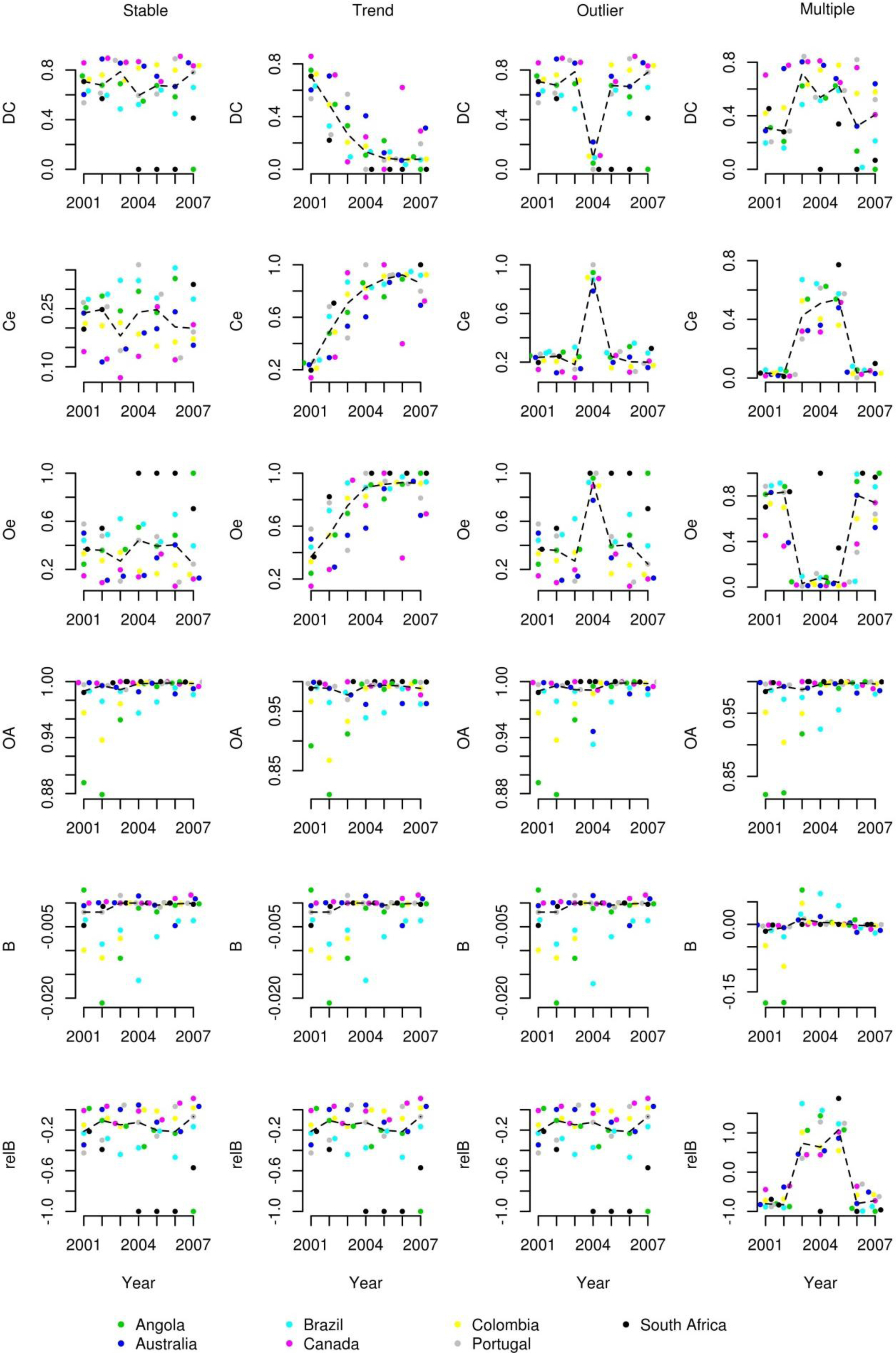
2.5. Hypothetical BA Products

To examine the performance of the proposed temporal stability analyses, we created four hypothetical BA products, where one hypothetical product was constructed to have temporal stability, while the other three products were constructed to have different departures from temporal stability, namely: (a) a decreasing trend in accuracy over time, (b) a single “outlier” year of different accuracy, and (c) multiple consecutive years of different accuracy. The starting point for each hypothetical BA product was the actual reference data for the seven study sites.
The first hypothetical product was named Stable and represented a product that possessed temporal stability. To construct this product, a map pixel was labeled as burned if more than half of the reference pixels within the map pixel were burned (the map pixel is labeled as unburned otherwise). Creating the map pixels in this fashion ensures a common misclassification structure for each year (although prevalence of BA can change year to year) because we retained the actual reference proportion (p+1) of each study site. This first hypothetical BA product should exhibit temporal stability.
The second hypothetical product was named Trend and represents a product that decreases in accuracy over time. Similarly to construction of Stable, a map pixel was labeled as burned if more than half of the reference pixels within the map pixel were burned. To create the decrease in accuracy, the map was offset one pixel east and one pixel south per year. This process would emulate a product with a very consistent classification algorithm but with a failure in the sensor data that is propagated over time as in the first year (2001) the drift is zero (i.e., all pixels are accurately spatially co-registered) and in the last year (2007) where there is a drift of six pixels east and six pixels south. The shift of pixels was implemented such that the proportion of burned pixels for the map (p1+) and reference (p+1) were unchanged. That is, the “column” of map pixels resulting from a one pixel shift of the map to the east would be re-inserted on the western edge of the boundary so that the map proportions p1+ and p2+ were not changed from prior to the shift. The reference map is not shifted at all so there was no change in p+1 and p+2. As B and relB were determined by the difference between p1+ and p+1, these measures take on the same values for the Trend BA product as they do for the Stable hypothetical product.
The third hypothetical product was named Outlier because it was constructed to represent a temporally stable product for all years except one. The initial map labels were created as described for the hypothetical BA product Stable, but for the year 2004 data, the map was offset by six pixels (thus, the outlier year, 2004, was equivalent to what was the year 2007 data in the Trend hypothetical product). The Outlier product emulates a product with a consistent classification algorithm but with a temporary (single year) failure in the sensor data.
The fourth hypothetical product was named Multiple and was designed to emulate a product with a temporally contiguous multi-year shift in accuracy. This product was constructed so that a different classification criterion was used for the central years (2003, 2004, and 2005). For 2003–2005, a map pixel was labeled as burned if more than 20% of the reference pixels within the map pixel were labeled as burned. For the other years (2001, 2002, 2006, and 2007), a map pixel was labeled as burned only if more than 80% of the reference pixels within the map pixel were labeled as burned. Multiple emulates a product with a temporary (three years) change of classification algorithm or sensor data that produces a change of sensitivity on detecting BA.

3. Results

The proportion of BA derived from the reference classification for each site and year provides important context to the assessment of temporal stability. Figure 2 shows the BA proportion (p+1) registered in the reference data for each site. A gradual decline in p+1 is observed over time, particularly for the maximum values. High p+1 values were registered in the reference data, particularly for Angola and Colombia during 2001 and 2002.

3.1. Hypothetical BA Products

The median (over the seven study sites) and individual site accuracy values for each year and each of the four hypothetical BA products are shown in Figure 3. If the temporal stability assessment is based on a larger sample of, for example, 25–30 sites, we recommend using a boxplot to display the quartiles, interquartile range, and outliers for each year instead of plotting only the individual site values. The graphical display of the median accuracy values over time for the four hypothetical BA products illustrates the temporal stability features created for these hypothetical products. Specifically, the Stable product shows only minor variation over time, the Trend product shows a strong downward trend in accuracy over time, the Outlier product shows the precipitous decline in accuracy for the single year, 2004, and the Multiple product reveals the higher accuracy created by construction for 2003–2005. The B and relB scores for Stable, Trend and Outlier, are identical by construction of these hypothetical products.
Table 2 shows the median values for the monotonic trend over time (b) for each of the six measures. Statistically significant trends (p-value < 0.05 level) on the “burned” category accuracy measures were detected for the hypothetical Trend product, which was constructed to have a decrease of accuracy over time. A statistically significant trend was also found for B in the Stable, Trend, and Outlier hypothetical products (by construction all three of these products have the same bias so the three significant tests represent in reality only a single test repeated three times). Although not purposely constructed as a feature of the hypothetical products, an increase in B over time from small negative values towards zero is observable from Figure 3 and this trend is statistically significant. The magnitude of the increase of B from small negative values towards zero is small (median of 0.0003, Table 2) indicating that the change in bias over time may not be large enough to substantively impact applications using these BA products.
The p-values derived from the Friedman test for the hypothetical products identified no statistically significant differences among years in OA for any of the four hypothetical populations (Table 3) emphasizing that OA is not a useful indicator of temporal stability. As would be desired, none of the other accuracy measures was statistically significant for the Stable product so the product constructed to possess temporal stability was identified by the analysis as being stable. The Trend and Outlier products had small p-values for the “burned” category accuracy measures DC, Ce, and Oe so these products were correctly identified as lacking temporal stability. Similarly, the Multiple product had statistically different accuracy measures over time for all measures except OA so this hypothetical product would have been correctly identified as lacking temporal stability.
The proportion of year-pairs with statistically significant differences (according to the Wilcoxon test) in one of the two measures of the “burned” category accuracy (DC and relB) was also successful at correctly identifying the temporal stability features designed into each hypothetical product. No significant differences were detected for the Stable product, but significant differences were found for the other three hypothetical products. For the Trend product, nine of the 21 year-pairs were statistically different and this result would be expected as adjacent years would not be expected to be different but pairs separated by more than one year would likely be statistically different. The six significant year-pairs for the Outlier product would be the differences between the outlier year and all six other years. For the Multiple product, we would expect 12 statistically significant year-pairs (each of the four low accuracy years different from each of the three high accuracy years) and these were in fact the significant differences identified by the Wilcoxon test.

3.2. Real BA Products

The median and individual site accuracy values for each year and each of the three real BA products (fire_cci, Globcarbon, and MCD64) are shown in Figure 4. Although OA is generally high for all three BA products, a striking feature of the data is that class-specific accuracy for “burned” is often low (i.e., high values of Oe and Ce accompanied by low values of DC). Because BA occupies such a small proportion of the landscape, it is not uncommon for omission error and commission error to be quite high because so little area is mapped as burned or is burned in the reference data. Another prominent feature of the data is that several very extreme values occur for individual sites and years for many of the accuracy measures. These outliers justify the use of the median instead of the mean to represent central tendency of the distribution because the median diminishes the influence of these extreme observations.
The formal statistical evaluation of temporal stability revealed no significant departures from temporal stability. The Wilcoxon test for a monotonic increase or decrease in accuracy over time was not statistically significant (α = 0.05) for any of the accuracy measures for any product (Table 4). From Figure 4, fire_cci appears to show an increase in DC over time, but the positive slope (median of 0.0276) resulted in a p-value of only 0.38. As noted in the Methods section, the lack of statistical significance of these tests may be attributable to the small sample size and high variability of the seven sample sites (i.e., low power).
The Friedman test, which evaluates the more general null hypothesis of equal median accuracy among all years, indicated some evidence for differences among years (Table 5). Although none of the real products have statistically significant changes in accuracy between years for DC and relB, the fire_cci product showed some evidence of a difference for Oe (p = 0.05) and B (p = 0.06) and the MCD64 product was found to have some evidence of a difference in B (p = 0.06).
The Wilcoxon tests evaluating whether DC or relB (for a given BA product) differed between two years revealed no statistically significant differences for MCD64. Three significant differences were identified for fire_cci (between 2002 and 2005, due to relB; between 2003 and 2007; and between 2004 and 2007, due to DC), and two significant differences were found for Globcarbon (between 2002 and 2006, due to DC and relB; between 2003 and 2006, due to relB). By design, these pairwise-year Wilcoxon tests are the most sensitive to departures of temporal stability (i.e., have the highest statistical power to detect a difference) and, as such, these tests are intended to alert users that these pairs of years may merit more detailed probing to determine if differences in accuracy might affect results of analyses that incorporate these years.

4. Discussion

The analysis of temporal stability should provide descriptive results of how accuracy is changing over time and to alert users to situations when temporal stability may be questionable. The analyses included an assessment of two different departures from temporal stability. The test for trend in accuracy over time is implemented to detect a patterned departure from temporal stability in the form of improving (or deteriorating) accuracy over time. The trend test would be sensitive to gradual improvement in accuracy over time whereas the second (i.e., Friedman) test assessing pairwise differences between years is designed to detect less patterned departures from temporal stability (i.e., discontinuities in accuracy over time). If temporal instability is detected from the analyses, a user would then need to decide if the variation in accuracy is substantively affecting results and whether to implement remedies that might alleviate the effects of temporal instability in accuracy. Our objectives did not include developing such remedies as these would be highly application specific. The methods described for assessing temporal stability are intended for applications in which the number of time periods is 5 to 15. For applications in which temporal stability is of interest for a much longer time series of data, methods taking advantage of the richer temporal database may be warranted.
Our proposed methodology uses statistical hypothesis testing, so the usual caveats of statistical hypothesis tests are relevant. For example, we have emphasized that for the illustrative results presented the statistical tests likely have low power because of the small sample size. If the sample size is small, failure to detect temporal instability (i.e., a non-significant test result) is not necessarily definitive evidence for temporal stability, but instead may be indicative of an inconclusive result because the small sample size is insufficient to yield an informative test. Conversely, if the sample size is very large, the statistical power will likely be high to detect even small variations in accuracy over time. A statistically significant finding of temporal instability (e.g., a difference in accuracy between two years) is not necessarily indicative of a practically important difference. If one of the nonparametric tests shows a statistically significant departure from temporal stability, it is important to examine the magnitude of the variation over time to evaluate subjectively if the departure from temporal stability could have practical ramifications on the applications using the BA products. For example, if the test for trend is significant, we would examine how much accuracy is increasing or decreasing per year to determine if the magnitude of the trend over time is substantial.
The importance of being able to assess temporal stability is highlighted by the case of the fire_cci product. Based on the tests for trend over time and the Friedman tests for differences in median accuracy between years, there was insufficient evidence to conclude that fire_cci suffered from temporal instability in accuracy. If these same test results were to occur for an assessment based on a larger sample size (i.e., more powerful statistical tests than were available for the sample size of seven sites), the fact that the fire_cci product did not exhibit a temporal trend in accuracy would be particularly interesting because fire_cci is based on data from different sensors whose availability varied over time. VGT was available for the whole time period (from 2001 to 2007), but ERS-ATSR was replaced by ENVISAT-AATSR in 2002, and MERIS was not available before 2005. This might cause variations in accuracy and/or in sensitivity, depending on the sensor data available. A lack of temporal instability in fire_cci would reflect that the procedures undertaken for merging of BA data from different sources were appropriate. The difficulties of merging BA data from different sources were noticed by Giglio et al. [4], who developed global, monthly BA estimates aggregated to 0.5° spatial resolution from MODIS BA maps and active fires.
The objective of evaluating temporal stability can be achieved by examining a sample of study sites purposely selected to provide broad representation of conditions of global BA. Generating reference BA perimeters is very demanding and a substantial investment of resources is needed to produce the reference datasets. Purposely selected study sites may be justified if the available resources can support only a small sample size. A better approach for evaluating temporal stability is to implement a probability sampling design [33] that incorporates a randomized rather than purposeful selection protocol. As noted in Section 2.1, a preferred option would be to select a stratified random sample of sites where the strata are biomes and to apply the methods for assessing temporal stability to each biome. The resources required to obtain a large enough sample (with multiple years of reference data) would be substantial and likely require a coordinated effort among the fire community to support such a task.

5. Conclusions

Temporal stability of accuracy is one of the most important features to be evaluated when a series of maps is produced over time, and the Committee on Earth Observing Satellites Land Product Validation Subgroup requires such an assessment to achieve Stage 2 validation of a product ( http://lpvs.gsfc.nasa.gov). Several methods to objectively evaluate temporal stability were developed. When applied to four hypothetical BA products, these methods successfully identified the patterns of temporal stability designed into the hypothetical BA products. The methods were then used to evaluate temporal stability of three real BA products, MCD64, Globcarbon and fire_cci. Although the statistical tests of temporal stability did not provide sufficient evidence to claim that any of the three real BA products was unstable through time, low statistical power attributable to small sample size may have contributed to the inability to detect departures from temporal stability in our illustrative analyses. Issues, such as power analysis and sample size determination, merit further investigation in the development of protocols to assess temporal stability. Future work should also focus on developing methods to reduce the processing time and effort required for generating the BA reference data and investigating sampling designs that might simultaneously serve two critical objectives, estimation, of descriptive accuracy of fire products and evaluation of temporal stability.

Acknowledgments

The authors would like to thank R. Cardoso, C. Sandow, S. Hantson, R. Ramo and D. Corti for their help with the generation of BA reference data, as part of the Fire Disturbance project (fire_cci), funded by the European Space Agency Climate Change Initiative. We would like to thank as well the reviewers for their valuable comments which helped to improve the quality of the manuscript.

Author Contributions

All authors have made major and unique contributions. M. Padilla is the main author who participated in the reference data generation, designed and processed the statistical analysis and wrote the draft version of the manuscript. S.V. Stehman gave valuable inputs on how accuracy should be measured, on the design of the temporal analysis and on the manuscript writing. J. Litago participated from early stages in the design of the temporal stability analysis, which is part of his expertise. E. Chuvieco, the principal investigator of the Fire Disturbance project, had the original idea and he supervised and participated with the work throughout all phases, from the reference data generation to the manuscript writing.

Conflicts of Interest

The authors declare no conflict of interest.

References

  1. Congalton, R.G.; Green, K. Assessing the Accuracy of Remotely Sensed Data: Principles and Applications; Lewis Publishers: Boca Raton, FL, USA, 1999; p. 137. [Google Scholar]
  2. Hollmann, R.; Merchant, C.; Saunders, R.; Downy, C.; Buchwitz, M.; Cazenave, A.; Chuvieco, E.; Defourny, P.; de Leeuw, G.; Forsberg, R.; et al. The ESA climate change initiative: Satellite data records for essential climate variables. Bull. Am. Meteorol. Soc 2013, 94, 1541–1552. [Google Scholar]
  3. Mouillot, F.; Schultz, M.G.; Yue, C.; Cadule, P.; Tansey, K.; Ciais, P.; Chuvieco, E. Ten years of global burned area products from spaceborne remote sensing—A review: Analysis of user needs and recommendations for future developments. Int. J. Appl. Earth Observ. Geoinf 2014, 26, 64–79. [Google Scholar]
  4. Giglio, L.; Loboda, T.; Roy, D.P.; Quayle, B.; Justice, C.O. An active-fire based burned area mapping algorithm for the MODIS sensor. Remote Sens. Environ 2009, 113, 408–420. [Google Scholar]
  5. Chuvieco, E.; Opazo, S.; Sione, W.; del Valle, H.; Anaya, J.; di Bella, C.; Cruz, I.; Manzo, L.; López, G.; Mari, N.; et al. Global burned land estimation in Latin America using MODIS composite Data. Ecol. Appl 2008, 18, 64–79. [Google Scholar]
  6. Roy, D.P.; Boschetti, L. Southern Africa validation of the MODIS, L3JRC, and GlobCarbon burned-area products. IEEE Trans. Geosci. Remote Sens 2009, 47, 1032–1044. [Google Scholar]
  7. Boschetti, L.; Flasse, S.P.P.; Brivio, P.A. Analysis of the conflict between omission and commission in low spatial resolution dichotomic thematic products: The Pareto Boundary. Remote Sens. Environ 2004, 91, 280–292. [Google Scholar]
  8. BAE Validation, GlobCarbon Demonstration Products and Qualification Report; ESA: Boeretang, Belgium, 2007; pp. 1–69.
  9. Tansey, K.; Grégoire, J.-M.; Defourny, P.; Leigh, R.; Pekel, J.-F.; Bogaert, E.; Bartholome, E. A new, global, multi-annual (2000–2007) burnt area product at 1 km resolution. Geophys. Res. Lett 2008, 35. [Google Scholar] [CrossRef]
  10. Latifovic, R.; Olthof, I. Accuracy assessment using sub-pixel fractional error matrices of global land cover products derived from satellite data. Remote Sens. Environ 2004, 90, 153–165. [Google Scholar]
  11. Campbell, J.B. Introduction to Remote Sensing, 2 ed; The Guilford Press: New York, NY, USA, 1996. [Google Scholar]
  12. Foody, G.M. Status of land cover classification accuracy assessment. Remote Sens. Environ 2002, 80, 185–201. [Google Scholar]
  13. GCOS, Guideline for the Generation of Datasets and Products Meeting GCOS Requirements; World Meteorological Organization: Geneva, Switzerland, 2010.
  14. Cohen, W.B.; Yang, Z.; Kennedy, R.E. Detecting trends in forest disturbance and recovery using yearly Landsat time series: 2. TimeSync—Tools for calibration and validation. Remote Sens. Environ 2010, 114, 2911–2924. [Google Scholar]
  15. Chuvieco, E. ESA CCI ECV Fire Disturbance—Product Specification Document; ESA Fire-CCI Project: Alcalá de Henares, Spain, 2013. [Google Scholar]
  16. Plummer, S.; Arino, O.; Ranera, F.; Tansey, K.; Chen, J.; Dedieu, G.; Eva, H.; Piccolini, I.; Leigh, R.; Borstlap, G.; et al. An Update on the GlobCarbon Initiative: Multi-Sensor Estimation of Global Biophysical Products for Global Terrestrial Carbon Studies. Proceedings of Envisat Symposium 2007, Montreux, Switzerland, 23–27 April 2007; ESA SP-636, pp. 1–8.
  17. Roy, D.; Jin, Y.; Lewis, P.; Justice, C. Prototyping a global algorithm for systematic fire-affected area mapping using MODIS time series data. Remote Sens. Environ 2005, 97, 137–162. [Google Scholar]
  18. Giglio, L.; Randerson, J.T.; van der Werf, G.R.; Kasibhatla, P.; Collatz, G.J.; Morton, D.C.; Defries, R. Assessing variability and long-term trends in burned area by merging multiple satellite fire products. Biogeosci. Discuss 2010, 7. [Google Scholar] [CrossRef]
  19. Bastarrika, A.; Chuvieco, E.; Martin, M.P. Mapping burned areas from Landsat TM/ETM+ data with a two-phase algorithm: Balancing omission and commission errors. Remote Sens. Environ 2011, 115, 1003–1012. [Google Scholar]
  20. Chuvieco, E.; Padilla, M.; Hantson, S.; Theis, R.; Snadow, C. ESA CCI ECV Fire Disturbance—Product Validation Plan (v3.1); ESA Fire-CCI Project: Alcalá de Henares, Spain, 2011. [Google Scholar]
  21. Boschetti, L.; Roy, D.; Justice, C. International Global Burned Area Satellite Product Validation Protocol. Part I—Production and Standardization of Validation Reference Data; Committee on Earth Observation Satellites: Maryland, MD, USA, 2009. [Google Scholar]
  22. Binaghi, E.; Brivio, P.A.; Ghezzi, P.; Rampini, A. A fuzzy set-based accuracy assessment of soft classification. Pattern Recognit. Lett 1999, 20, 935–948. [Google Scholar]
  23. Stehman, S.V.; Arora, M.; Kasetkasem, T.; Varshney, P. Estimation of fuzzy error matrix accuracy measures under stratified random sampling. Photogramm. Eng. Remote Sens 2007, 73, 165–174. [Google Scholar]
  24. Fielding, A.H.; Bell, J.F. A review of methods for the assessment of prediction errors in conservation presence/absence models. Environ. Conserv 1997, 24, 38–49. [Google Scholar]
  25. Forbes, A.D. Classification-algorithm evaluation: five performance measures based on confusion matrices. J. Clin. Monit 1995, 11, 189–206. [Google Scholar]
  26. Fleiss, J.L. Statistical Methods for Rates and Proportions; John Wiley & Sons: New York, NY, USA, 1981. [Google Scholar]
  27. Hand, D.J. Discrimination and Classification; John Wiley and Sons: New York, NY, USA, 1981. [Google Scholar]
  28. Meredith, M.P.; Sethman, S.V. Repeated measures experiments in forestry: Focus on analysis of response curves. Can. J. Forest Res 1991, 21, 957–965. [Google Scholar]
  29. Friedman, M. The use of ranks to avoid the assumption of normality implicit in the analysis of variance. J. Am. Stat. Assoc 1937, 32, 675–701. [Google Scholar]
  30. Chou, Y.H.; Minnich, R.A.; Chase, R.A. Mapping probability of fire occurrence in San Jacinto Mountains, California, USA. Environ. Manag 1993, 17, 129–140. [Google Scholar]
  31. Griffith, D. Spatial Autocorrelation. In International Encyclopedia of Human Geography; Kitchin, R., Thrift, N., Eds.; Elsevier: New York, NY, USA, 2009; pp. 1–10. [Google Scholar]
  32. Sheskin, D.J. Handbook of Parametric and Nonparametric Statistical Procedures; Chapman & Hall/CRC: Boca Raton, USA, 2004. [Google Scholar]
  33. Stehman, S.V. Sampling designs for accuracy assessment of land cover. Int. J. Remote Sens 2009, 30, 5243–5272. [Google Scholar]
Figure 1. Study sites (black squares) and burned area from 2001 to 2007 at 0.5° spatial resolution from the Global Fire Emissions Database version 3 [4,18].
Remotesensing 06 02050f1
Figure 2. BA proportion according the reference data (p+1) in the dataset of each study site and year. Some points are displaced along the x-axis such that no points overlap.
Remotesensing 06 02050f2
Figure 3. DC, Ce, Oe, OA, B, and relB values of each study site and year for the hypothetical products. Some points are displaced along the x-axis such that no points overlap. Yearly median values are represented with a dotted line.
Remotesensing 06 02050f3
Figure 4. DC, Ce, Oe, OA, B, and relB values of each study site and year for the real BA products. Some points are displaced along the x-axis such that no points overlap. Yearly median values are represented with a dotted line.
Remotesensing 06 02050f4
Table 1. Error matrix for a study site for a BA product where pij is the proportion of area in cell (i, j) (see Equation (1)).
Reference data
Global ProductBurnedUnburnedRow total
Burnedp11p12p1+
Unburnedp21p22p2+
Col. Totalp+1p+2p = 1
Table 2. Median values of the trend over time (b) for the sample of seven study sites and the four hypothetical products. “*” refers to a statistically significant test result (median slope different from zero) at α = 0.05 according the Wilcoxon test.
ProductDCCeOeOABrelB
Stable−0.00210.0033−0.00020.00080.0003 *0.0163
Trend−0.0889 *0.1054 *0.0781 *0.00120.0003 *0.0163
Outlier−0.00210.0033−0.00020.00080.0003 *0.0163
Multiple−0.00490.01120.00310.00100.00150.0064
Table 3. Friedman test p-values for the hypothetical products for the accuracy measures (p-values less than 0.05 indicate strong evidence that not all years have the same median accuracy).
ProductDCCeOeOABrelB
Stable0.880.900.720.510.160.60
Trend<0.0010.002<0.0010.710.160.60
Outlier0.040.060.030.460.160.60
Multiple0.003<0.001<0.0010.64<0.001<0.001
Table 4. Median values of the trend over time (b) of the accuracy measures for the three BA products (Wilcoxon p-values > 0.05 in all cases).
ProductDCCeOeOABrelB
fire_cci0.0276−0.0016−0.0381−0.00060.00380.0971
Globcarbon−0.0026−0.01320.00570.0013−0.0002−0.0642
MCD64−0.01000.0221−0.00200.00050.0019−3e–5
Table 5. Friedman test p-values (values less than α = 0.05 would indicate strong evidence that not all years have similar median accuracy values).
ProductDCCeOeOABrelB
fire_cci0.140.870.050.540.060.35
Globcarbon0.240.490.270.500.970.21
MCD640.730.540.550.450.060.23

