Article

Forest Delineation Based on Airborne LIDAR Data

1
Institute of Photogrammetry & Remote Sensing, Vienna University of Technology, Gußhausstraße 27-29, A-1040 Vienna, Austria
2
Department of Forest Inventory at the Federal Research and Training Center for Forests, Natural Hazards and Landscape, Seckendorff-Gudent-Weg, A-1130 Vienna, Austria
*
Author to whom correspondence should be addressed.
Remote Sens. 2012, 4(3), 762-783; https://doi.org/10.3390/rs4030762
Submission received: 18 January 2012 / Revised: 7 March 2012 / Accepted: 8 March 2012 / Published: 20 March 2012
(This article belongs to the Special Issue Laser Scanning in Forests)

Abstract

:
The delineation of forested areas is a critical task, because the resulting maps are a fundamental input for a broad field of applications and users. Different national and international forest definitions are available for manual or automatic delineation, but unfortunately most definitions lack precise geometrical descriptions for the different criteria. A mandatory criterion in forest definitions is the criterion of crown coverage (CC), which defines the proportion of the forest floor covered by the vertical projection of the tree crowns. For loosely stocked areas, this criterion is especially critical, because the size and shape of the reference area for calculating CC is not clearly defined in most definitions. Thus current forest delineations differ and tend to be non-comparable because of different settings for checking the criterion of CC in the delineation process. This paper evaluates a new approach for the automatic delineation of forested areas, based on airborne laser scanning (ALS) data with a clearly defined method for calculating CC. The new approach, the ‘tree triples’ method, is based on defining CC as a relation between the sum of the crown areas of three neighboring trees and the area of their convex hull. The approach is applied and analyzed for two study areas in Tyrol, Austria. The selected areas show a loosely stocked forest at the upper timberline and a fragmented forest on the hillside. The fully automatic method presented for delineating forested areas from ALS data shows promising results with an overall accuracy of 96%, and provides a beneficial tool for operational applications.

Graphical Abstract

1. Introduction

In recent years, the increasing use of forest products derived from airborne laser scanning (ALS) data as well as many ongoing projects related to this topic show the high demand for this research field. Different products like, e.g., estimated tree heights [13], growing stock estimations [4,5], or forest structure analyses [6,7] are of interest for a broad field of applications and users (e.g., forestry, biologists, risk management for natural hazards). An overview of current methods for extracting forest parameters from ALS is given in Hyyppä et al. [8]. The results determined from these applications are highly dependent on the fundamental input parameters’ size and position of the delineated forest areas. The delineation of these areas is therefore a crucial task. The size of forested areas is also of interest for governmental authorities (e.g., taxation, financial support of the European Commission) and, in a broader sense, for politics (e.g., greenhouse gases, Kyoto protocol).
The delineation of forests has a long tradition in remote sensing. In the past, mainly aerial images were used for a manual or semi-automated extraction of forested areas. Shadow effects limit this task, particularly for detecting small forest clearings and the exact delineation of forest borders. Additionally, the quality of the results of a manual delineation is subjective and variable between analysts and may lead to inhomogeneous, maybe even incorrect datasets. In particular, in loosely stocked areas, the delineated results show low quality. To classify an area as forest or non-forest, different national forest definitions are available [9], beside a global definition of the Food and Agriculture Organization of the United Nations (FAO) [10,11]. To delineate forested areas, an exact geometric forest definition is required. Unfortunately, the current forest definitions are imprecise in most cases. For example, the criterion of crown coverage (CC) is fundamental and mandatory. With regard to the forest definition given by European Commission, the criterion of minimum area is the second important criterion. CC, also known as vertical canopy coverage [12], or forest canopy cover, is defined as the proportion of the forest floor covered by the vertical projection of the tree crowns [13]. Most of the common forest definitions lack precise geometric descriptions for calculating CC (e.g., the reference size and shape for which the amount of projected crown area is calculated). Therefore, the results of current forest delineations are often not comparable and make the CC a doubtful criterion. In recent years, fully automated methods for a forest delineation, based on aerial images or ALS data, have been proposed. They can overcome the limitations of manual delineation in most instances and produce user independent results in short evaluation times.
Radoux et al. [14], for example, use different very high resolution multispectral satellite images to delineate forest stands in Belgium. They use an automatic segmentation to delineate homogeneous land cover objects, based on the orthorectified images from IKONOS-2 and SPOT-5. Unfortunately, no criteria of a forest definition are treated.
Mustonen et al. [15] evaluate the applicability of a canopy height model (CHM), derived from ALS data, for an automatic segmentation of forest stands in Finland. Additionally, they evaluate a segmentation based on the CHM combined with aerial images. For the delineation of stands based on the CHM, the height information of forest stands is used as a fundamental input. The authors mention that the use of other parameters, such as number of stems per hectare or canopy cover, both derived from ALS, could be an improvement. However, the method of Mustonen et al. [15] focuses on delineating forest stands inside forested areas.
Wang et al. [16,17] use aerial images together with ALS data for the automatic delineation of forested areas in Switzerland. They use a green vegetation index, derived from the red and green spatial bands of orthophotos, in combination with a height thresholded canopy height model (CHM), derived from ALS data, to classify forest candidate pixels from the images. In a next step, they apply an image segmentation to find homogeneous, independent regions. By checking the curvature of each segment based on the CHM, forested areas are found. Unfortunately, Wang et al. do not treat the criterion of CC, which is a mandatory criterion in the Swiss forest definition [18].
Straub et al. [19] delineate forested areas in Germany, based on the normalized digital surface model (nDSM) derived from ALS data. Furthermore, they use point density maps to derive a normalized image, which is thresholded to find areas (pixels) covered by vegetation. Based on these areas, they classify into forest vegetation and non-forest vegetation. For this classification, the criteria height, CC, area and width are used. The reference areas for checking the CC criterion are extracted by intersecting vegetation pixels above 3 m with a grid of 20 × 20 m. In the resulting, individually shaped areas, pixels lower than 5 m in the nDSM are summed. The relation between reference area and summed pixels represents the amount of CC. Regions with a CC value greater than 50% are connected and checked against the minimum area criterion of 1,000 m2. Finally, the minimum width is checked by “skeletonization” and by analyzing profiles of the resulting areas. Unfortunately, Straub et al. [19] do not explain why they use a square shaped grid with a grid size of 20 × 20 m for checking the CC criterion. As discussed in Eysn et al. [20], different settings for the grid size lead to different results.
As summarized in the three examples from Finland, Switzerland and Germany, forest is delineated with different methods and parameter settings from ALS data and orthophotos. This is critical because delineation results based on different definitions need to be compared. For example, the Global Forest Resources Assessment (FRA) is based on data (e.g., the amount of forested areas) that countries provide to the FAO in response to a common questionnaire every 5 to 10 years. The FAO analyzes this information and presents the current status of the world’s forest resources and their changes over time [21]. Because taxation is also strongly related to the amount of forested areas, a clear forest definition and consequently technically correct forest delineation are crucial.
In the approach here presented, the forested areas are automatically delineated, based on ALS data and considering the forest definition of the Austrian national forest inventory (NFI). As shown in Eysn et al. [20], different settings for reference size and shape within the CC calculation process lead to different delineation results. Therefore, the focus is laid on implementing the criterion of CC in a comprehensible, geometrically clearly defined way to be able to produce comparable delineation results. The used forest definition is mainly based on the five criteria (1) minimum tree height (2) minimum CC (3) minimum forest area (4) minimum forest area width and (5) land use [22]. In the approach here presented, criteria one to four are treated.
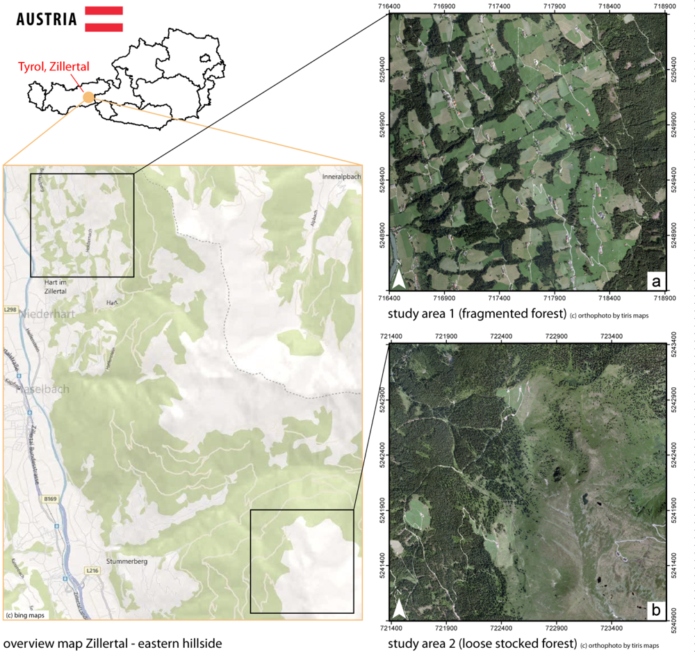
The remaining parts of this paper are organized as follows: Section 2 describes the selected study areas and the used data. Section 3 describes the methodology and implementation, whereas results are presented and discussed in Section 4. Finally, concluding remarks are given in Section 5. This special issue paper is based on two conference papers by Eysn et al. [20,23].

2. Study Areas and Data

2.1. Study Areas

In this contribution, two different study areas in the Zillertal, which is located in the eastern part of the federal state of Tyrol, Austria, are investigated. Each study area covers an area of 2.5 × 2.5 km2 and shows different structures and amounts of forested land (Figure 1).
Study area 1 consists of a fragmented forest with patchwork forest stands on the hillside (Figure 1(a)) with elevations from 600 to 1,600 m above sea level (a.s.l.) Study area 2 consists of a loosely stocked forest at the upper timberline (Figure 1(b)) with elevations from 1,800 to 2,000 m a.s.l. The dominant tree species in both study areas are coniferous trees such as Norway Spruce (Picea abies) and European Larch (Larix decidua). Beside the forested areas, artificial objects, such as buildings and power lines, can be found in the study areas.

2.2. Airborne Laser Scanning Data

Topographic data were acquired using the discrete Airborne Laser Terrain Mapper ALTM 3100, manufactured by Optech Inc. The data acquisitions were done in the framework of a commercial terrain-mapping project, fully covering the Federal State of Tyrol. The ALS data and the digital terrain model (DTM) were provided by the “Amt der Tiroler Landesregierung, Gruppe Landesbaudirektion, Abteilung Geoinformation”. For the two study areas, the ALS data were acquired during multiple flight campaigns in 2008 under leaf-off and leaf-on canopy conditions without snow cover. The mean point density is about 5 echoes/m2 for study area 1 and 4 echoes/m2 for study area 2. The ALS data were delivered as XYZ coordinate triples (georeferenced in UTM-32), organized in flight strips, and classified to first echoes (FE) and last echoes (LE). Single echoes are classified as LE. For further calculations, FE and LE were merged and the data organized in 2.5 × 2.5 km tiles. Details of the ALS data used are summarized in Table 1. For the DTM generation the hierarchic robust filtering approach described in Kraus and Pfeifer [24] was applied. The DTM has a spatial resolution of 1 × 1 m2.

2.3. National Forest Inventory Data

For the delineation of forested areas, a statistical relationship between tree height and crown radius are computed, based on measurements of crown radii from the Austrian national forest inventory (NFI). The NFI data were acquired by the Department of Forest Inventory of the Federal Research and Training Center for Forests, Natural Hazards and Landscape (BFW), in the framework of the ongoing NFI. The delineation of forested areas in alpine regions is most critical in sparsely stocked forests, which mainly occur at the upper timberline at high elevations. Therefore, a subsample of measured trees in Tyrol, Austria was chosen for describing the crown radii for trees with low competition according to a border situation. Only trees of the species European Larch (Larix decidua), Swiss Stone pine (Pinus cembra) and Norway Spruce (Picea abies L.) were selected because they are relevant and representative of loose areas around the upper timberline in the study areas. Thus, dense stands and trees of lower social classes according to Kraft [25] were excluded. A short description of the data used is given in Table 2.

3. Methods

The delineation of forested areas is commonly a large area application. Performing this task on a pure pointcloud basis would be very extensive because of the large amount of data, which arises when working with high-density laser point data. Therefore, the focus of this work was to develop a method based on the rasterized ALS data. In addition to the ALS point clouds, most of these base products, such as DTM and the digital surface model (DSM), are available with a spatial resolution of 1 × 1 m for all federal states in Austria.
As described in Section 1, only the geometrical criteria of the Austrian NFI (min. area, min. height, min. width and min. crown coverage) are used for the delineation of forested areas. Land use criteria are not considered in this study. It has to be clarified that land use and legal restrictions are in most cases not deducible from ALS data. Other data sources, such as the cadastre, are needed to gather this information. From a hierarchical point of view, the four geometrical criteria of the Austrian NFI have equal rights. To apply these criteria to remote sensed data, a hierarchy has to be defined with respect to a processing chain. For instance, it would make no sense to check the minimum forested area if there is no potential area detected yet. In this approach, the hierarchy is defined as follows: (1) min. height, (2) min. CC, (3) min. area and (4) min. width, whereas (3) and (4) are checked in an iterative process.

3.1. Derived Base Products

In a preliminary working process, two base products were calculated from the pointcloud. The first one is the nDSM, which is derived by subtracting the DTM from the DSM. The nDSM, also known as CHM, is a very suitable product for the delineation of forested areas because it directly shows object heights (e.g., tree heights). In order to process the DSM, a land-cover-dependent derivation approach, described in Hollaus et al. [26], was chosen. This approach makes use of the strengths of different algorithms for generating the final DSM by using surface roughness information to combine two DSMs, which are calculated based (i) on the highest echo within a raster cell and (ii) on moving least squares interpolation (i.e., moving planes interpolation). The second base product is a slope adaptive echo ratio (sER) map, which is calculated, based on the 3D point cloud using FE and LE ALS data. As described in Höfle et al. [27,28], the sER is defined as the ratio between the number of neighboring echoes in a fixed search distance of 1.0 m measured in 3D (a sphere) and all echoes located within the same search distance in 2D (a cylinder). The sER is a measure for local transparency and roughness of the top-most surface and is well suited for the elimination of artificial objects in the forest delineation process (see Section 3.2). The base products derived have a spatial resolution of 1 × 1 m2 and have been processed consistently for all study areas using the OPALS software [29].

3.2. Removing Artificial Objects

Since all elevated objects, e.g., buildings, forests, power lines and cable cars, are present in the nDSM, a pre-processing step is required to extract a vegetation mask that includes potential forested areas. As shown in previous studies [27,
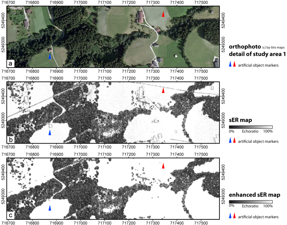
30], the sER can be used to differentiate between buildings and forested areas. A sER value of 100% means that the echoes within the 2D search radius describe a planar surface (e.g., roofs), whereas a sER value lower than 100% means that the echoes are vertically distributed within the 2D search area, thus indicating penetrable objects, i.e., forests. A specialty of the sER is that the outer edges of buildings as well as power lines appear as pixel lines with values lower than 100% in the sER maps (see figure in Section 4.2). This is the case because echoes that are vertically distributed on walls of buildings and in the area of power lines wrongly indicate penetrable objects. Therefore, an empirically determined threshold of 85% is applied to the sER map for eliminating artificial objects. Furthermore, morphological operations (opening, closing) are applied to remove the remaining building borders and power lines. The resulting vegetation mask provides a fundamental input for the delineation of forested areas.

3.3. Minimum Height Criterion

The minimum height criterion is not well defined in the Austrian NFI, since it is dependent on an “in situ reachable tree height”. Depending on this in situ reachable tree height, which obviously has to be defined by user-dependent expert knowledge, the minimum tree height can be set to 2–7 m. Reachable tree heights cannot be obtained from ALS data directly. However, as the goal of this approach is a user independent result, a minimum tree height of 2.0 m is used for the automatic delineation process. The minimum height criterion is applied by height thresholding the nDSM within the vegetation mask.

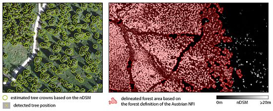
3.4. Minimum Crown Coverage Criterion

The parameter CC defines the vertically projected crown area of trees within a certain reference area. Current automatic methods for calculating CC maps are commonly based on a moving window approach. The kernel size of the moving window, which defines the reference area, is a fundamental parameter. Since there is no exact definition of the size and the shape of the reference area available in the NFI, different results are derived if different kernel sizes and shapes (e.g., square, circle) are applied [21]. Another limitation of the moving window approach is that smoothing effects occur at the border of a forest and at small clearings. To overcome these limitations, a new unambiguous approach for determining CC is presented. The method developed aims to define the criterion of CC with a clear geometrical definition, which is based on ALS and NFI data. The basic idea is to express CC as a relation between the sum of the crown areas of three neighboring trees and the area of their convex hull (Figure 2).

3.4.1. Potential Tree Positions

The potential tree positions are detected with a local maxima filter applied to the nDSM. A circular kernel with an empirically determined size of 5 × 5 m [23] is used to determine potential tree positions. The chosen properties of the local maxima filter are optimized for trees at the timberline, because those areas are the most critical ones for the CC criterion. The detected positions are restricted, to be found within valid areas of the vegetation mask, as well as within valid areas of the height-thresholded nDSM.

3.4.2. Tree Crown Estimation

The crown radii Ri are assessed using the following empirical function, describing the relationship between tree height and crown radius:
R i + a + b t i + c e i
The input parameters for this function are the tree heights ti (z-value of the nDSM at the detected potential tree position) and the elevation of the tree ei (z-value of the DTM at the detected potential tree position). The coefficients a, b and c are calibrated, based on sample crowns. For this calibration the following two possibilities are investigated:
  • Measurements of crown radii from the NFI are used for the calibration. For this study the function was calibrated for trees near the timberline. Tree crowns, tree heights and elevations of sample trees, measured within multiple field campaigns of the Austrian NFI (Section 2.3), are used to calibrate the coefficients a, b and c in Equation (1). The calibrated function is applied to the detected tree positions to estimate the crowns for all trees within the study areas.
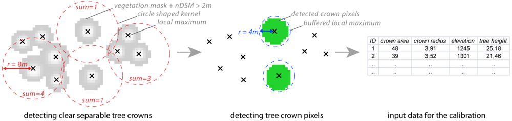
  • Clearly separable tree crown samples are automatically extracted from the nDSM to calibrate the function. The main idea is to extract only trees which are located at least 8 m away from any other detected tree. The distance of 8 m is empirically determined for the study areas and represents the largest tree crown diameter found in the study areas. Based on the tree crowns of those filtered trees the function is locally calibrated (Figure 3). The sample trees are detected with a moving window approach, based on a binary raster map of the local maxima. Pixels in the resulting map, where the sum of all pixels within a circular kernel with a radius of 8 m is one, provide positions of trees with a clear, separable crown. The broadest crown diameter is found by applying the NFI calibrated function to the detected local maxima. The positions found are buffered by half of the previously-used kernel size and are intersected with the height thresholded nDSM (nDSM ≥ 2 m) and the vegetation mask. The resulting binary map shows the crown pixels of the identified sample trees. For each tree, the crown area is extracted from the map, and furthermore the average crown radius is derived. Additionally, the tree height and elevation of each sample tree is extracted from the nDSM and the DTM respectively at the position of the corresponding local maximum. For each study area the coefficients of Equation (1) are estimated by solving the system of linear equations based on the crown radii provided, tree heights and elevations of the sample trees. Finally, for each study area the locally calibrated function is applied to derive the crown radii for all trees.
To validate the estimated crowns for both possibilities, the derived crown areas are compared to the source map. The source map for the calculations is the height-thresholded nDSM (nDSM > 2 m) intersected with the vegetation map. In the source map, all pixels fulfilling the selected threshold are assumed to represent a crown pixel. For each study area the sum of these pixels represents the amount of land covered by tree crowns. To perform a clear validation of the estimated tree crowns, only crown pixels from detected trees should be investigated; otherwise crown pixels of non-detected trees or artificial objects such as buildings and power lines would distort the validation. For that reason the detected local maxima positions are buffered by half of the biggest tree crown diameter found in the study areas to limit the crown pixel to the tree crowns that are represented by detected local maxima. These remaining crown pixels are summed and represent the reference crown area. Furthermore, the areas of the estimated crowns are also summed for each study area and calibration method and compared with the reference crown area.
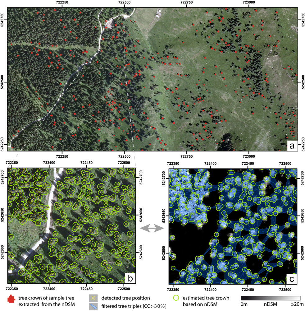
3.4.3. Tree Triples

To connect three neighboring trees, a Delaunay triangulation is applied to the previously-detected tree positions. Since the nearest neighbor graph is a subgraph of the Delaunay triangulation, the three closest standing trees are connected and the minimum inner angles of the triangles are maximized to provide non-sharp-angled triangles, if possible. Further details on Delaunay triangulations can be found in Fortune [31] or Isenburg et al. [32]. The Delaunay triangulation is calculated using libraries of the software CGAL [33].

3.4.4. CC Calculation

In a next step, the sum of the crown areas Acr of three neighboring trees and the area of their convex hull Ahull is calculated for each tree triple. For this purpose, a tool was implemented in Python [34], which imports a triangulation, calculates the parameters Acr and Ahull and returns the CC value for each tree triple. For overlapping tree crowns within a tree triple, the area of the union of crowns is used for Acr. The derived CC values are assigned to their associated triangles. In a next step, the selected CC threshold of 30% is applied to the triangulation and triangles, which do not fulfill the threshold, are removed. As the exported result is an edited triangulation with triangles fulfilling the CC criterion, the borderlines of the derived map represent the tree stem axes and not the convex hulls of the tree triples (Figure 4). For this reason, a borderline correction is applied by buffering the resulting map by the maximum available crown radius found in the study area. In order to prevent an overestimation of the derived potential forest mask, the buffered area is intersected with the vegetation mask and the resulting areas are added to the valid areas of the edited triangulation. The result of these calculations is a potential forest mask that considers the minimum height criterion as well as the minimum CC criterion.

3.5. Minimum Area Criterion

The minimum area criterion is applied by using standard GIS-queries. The areas of all valid polygons are calculated for the potential forest mask fulfilling the height- and CC-criterion. Firstly, gaps within polygons are checked. If the gap is smaller than 500 m2, the gap is filled. Secondly, the polygons themselves are checked. All polygons that do not fulfill the minimum area criterion of 500 m2 are erased.

3.6. Minimum Width Criterion

The minimum width criterion of 10 m is applied by using morphologic operations (open, close) based on the intermediate result fulfilling the criteria height, CC and area. For this operation, a circular kernel with a radius of 5 pixels (pixel size 1 × 1 m) is used to eliminate narrow forested areas that do not fulfill the criterion. This operation is also related to the area criterion, because the removal of narrow areas leads to changes of the forested areas. Therefore, an iterative process of checking minimum area and width is applied.

3.7. Validation

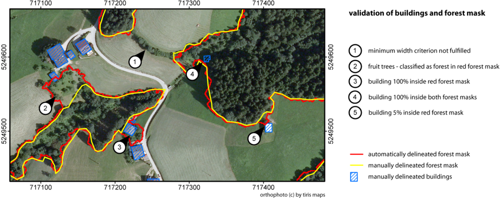
The validation of the final forest mask is performed for the study area 1 (fragmented forest) by comparing the automatically-delineated mask to a reference mask. The reference mask is manually interpreted, based on an orthophoto, using the criteria of the Austrian NFI. The orthophoto was acquired in July 2009 and has a spatial resolution of 0.2 m.
To validate the automatically delineated forest mask with respect to the footprint areas of buildings covered by the forest mask, a building layer is created by manually delineating buildings, based on an orthophoto. Because the acquisition date of the orthophoto differs from the acquisition date of the ALS data, the delineated buildings might be incorrect, or even incomplete, as a result of changes. Therefore, the sER map was used as an additional input within the delineation process to update the building polygons, as necessary. Buildings within densely forested areas might be overgrown and therefore not visible in the orthophoto or sER map. To acquire information about such buildings, the cadastre is used as a third input to gain completeness. For both study areas, the delineated building polygons are intersected with the final forest mask. The remaining building polygons are analyzed.

4. Results and Discussion

4.1. General Considerations

The crowns in the derived base products of ALS tend to be overestimated, because the base products are commonly raster-based and the exact size of the modeled crowns depends on the spatial resolution of the models and on the method applied to calculate the DSM.
Reference forest maps for large areas, especially those with a high degree of detail, are hard to obtain from other remote sensing data or from in situ measurements. In particular, for loosely stocked forests, manually-delineated forest maps based on orthophotos are very limited in quality and always depend on the operator. Therefore, the validation of the automatically delineated forest mask could only be performed for the fragmented study area, since no manually interpreted reference map is available for the loosely stocked study area.
In the following sections, the results of the previous calculations are presented and discussed:

4.2. Removing Artificial Objects

The results of the method described in Section 3.1 are shown in Figure 5 for study area 1. Figure 5(b) shows the original sER-map with colored markers pointing to selected artificial objects. Figure 5(c) shows the enhanced sER-map. The applied processing chain leads to suitable results for eliminating artificial objects and for deriving the vegetation mask. Buildings, power lines, cable cars, etc. are removed from the sER-map in most instances, while green areas with a sER value lower than 85 are retained. The vegetation mask obtained is used as a spatial limitation for further processing steps.

4.3. Forest Delineation

4.3.1. Detection of Potential Tree Positions

A manual inspection of the automatically detected potential tree positions based on the nDSM and the orthophoto shows suitable results (Figure 6(b)). Due to the limitation of the maxima search of the vegetation mask, no erroneous tree positions at building borders, roof ridges or power lines are available. Because of the small kernel size of 5 × 5 pixels, multiple local maxima are sometimes found within the area of large single tree crowns. In particular, within densely forested areas, the detected local maxima do not represent the exact tree stem positions and the tree detection rate can be low. Single and clearly separable trees in loosely stocked areas, e.g., near the timberline, are correctly detected in most cases. In general, it can be stated that the completeness of detected local maxima depends on the chosen kernel size, the kernel shape and the tree crown shape. With respect to the estimation of CC, inexact or non-detected trees below dominant trees within a dense forest play a negligible role. Since the CC criterion of forest inventory definitions is commonly in the range of 5% to 50%, the most critical areas are covered with sparse, loosely stocked forests, where primarily single trees are present. Such trees are clearly separable even with a rather simple local maxima filter.

4.3.2. Tree Crown Estimation

For the detected local maxima, the corresponding tree crowns were calculated, based on the calibrated equations determined from NFI data and the nDSM respectively. For each sample tree the crown radius, the tree height and the DTM height were used. The calibrated coefficients of Equation (1) for calculating the crown radii can be found in Table 3.
For the calibration based on the nDSM without NFI data, Equation (1) was calibrated with sample trees detected in the nDSM. For the loosely stocked forest (study area 2), 1,633 tree crowns, and for the fragmented forest (study area 1), 843 tree crowns could be extracted from the nDSM. The extracted tree crowns are found in loosely stocked areas as well as in denser forested areas. A visual inspection of the extracted sample crowns with an orthophoto shows a good agreement for the detected crowns and the distribution of the samples around the study areas (Figure 6(a)). Only tree crowns, where just a single local maximum was detected within a tree crown, were extracted by the algorithm. The calibrated coefficients for each study area can be found in Table 4.
The validation of the estimated tree crowns for the fragmented study area 1 shows an overestimation of 5% and an underestimation of 25% if the tree crown model is calibrated, based on the nDSM and the NFI data respectively (Table 5). The underestimation of the crowns, estimated based on NFI data, might occur from the very widespread tree samples used in different situations. Additionally, these samples are limited to three tree species which might be more specific to the timberline than to the hillside. Furthermore, the tree samples used are distributed over the entire federal state of Tyrol. Therefore, the calibrated model represents an average tree crown size.
For the loose stocked study area 2, the crown estimation based on the nDSM shows an overestimation of 10%, with the estimation based on NFI data showing an underestimation of 10%. The overestimation might be due to the fact that in the loosely stocked area more trees are detected than in denser areas and tree crowns of single trees in the open terrain tend to be larger than in dense areas, due to the improved sunlight conditions.
The calibrated functions are plotted in Figure 7 for both study areas. Elevations of 1,500 m a.s.l. and 2,000 m a.s.l. are chosen for the fragmented and loosely stocked study areas respectively for plotting the functions. In contrast to the NFI function, the loosely stocked study area the calibrated function based on the nDSM shows a better agreement than the function for the fragmented study area. The bigger difference of the functions for the fragmented area shows the limitations of a NFI function that was calibrated for a usage at the upper timberline when used in other areas. This also corresponds to the huge underestimation of 25% of the NFI function applied to the fragmented study area. A locally calibrated function can overcome these limitations.
Since the calibration based on the nDSM is not always sufficient (e.g., if too few sample trees are extracted in the current study area: if the equation systems of the samples are non-solvable) the calibration based on NFI data is equally necessary. A combination of both might be a good solution. If the local calibration of the function fails, the NFI calibration is used or vice versa. If no NFI data are available or only the nDSM calibration should be used, an extension of the current study area can help if the calibration based on the nDSM fails. With an increasing area, the probability to find single trees increases. Since the crowns, estimated based on the nDSM, fit better for our study areas, the corresponding functions are used for the tree crown estimation in the delineation process.

4.3.3. Tree Triples

The Delaunay triangulation of the potential tree positions shows conclusive results for the connection of tree triples. The detected tree triples are reliably filtered and eliminated, depending on the selected CC threshold (Figure 6(c)). In particular, in loosely stocked areas at the forest timberline, this method provides a suitable and reproducible potential forest mask. This mask is a fundamental input for the final delineation of forested areas based on a forest definition. Because the tree detection rate is limited in dense stocked forests, the “CC map” based on tree triples shows less detail for such areas. As this method is optimized for loosely stocked forests, it does not provide a highly detailed crown coverage map for dense forests. However, this lower detail in dense areas has no effect on the forest area delineation, because common forest definitions use a CC threshold lower than 50% and therefore the focus is only on looser stocked forests.

4.3.4. Final Forest Mask

In Figure 8 the results for the automatic delineation of the forested areas are. The delineation result for the loosely stocked forest (Figure 8(a)) shows a very jagged forest mask at the upper timberline. Since there is no clearly defined forest border, as in denser forested areas at lower elevations, this result is feasible. Only forested areas are detected by the algorithm, since none of the 22 existing buildings are considered as forest. Single trees on the open terrain as well as areas that are too loosely stocked are reliably excluded from the forest mask. Compared to a manual interpretation, the presented approach is fully automated, the results are independent from the operator and therefore reproducible.
The resulting forest map for the fragmented forest (Figure 8(b)) shows a good agreement with a manual inspection of the forested areas based on an orthophoto and the nDSM. A validation with the manually delineated reference mask shows a producer’s accuracy of 97% and a user’s accuracy of 94% for the classified forest areas (Table 6). The overall accuracy is 96% with a Kappa of 0.92. Due to the applied minimum area criterion, small forest patches with an area less than 500 m2, are removed, and forest clearings with an area less than 500 m2 are assigned to the forest area. As the preliminary output of the tree triples approach represents the forests borderline along the tree axis, the borderline-corrected forest area delineates the real forest area with good accuracy (Figure 9). Narrow forest areas are eliminated by applying the minimum width criterion (Figure 9, Marker 1). Figure 9, Marker 2 shows an area planted with fruit trees that was wrongly detected by the algorithm. Since the method presented only uses geometrical criteria, additional parameters such as tree species or land use would be needed to tackle this problem. The validation of the automatically delineated forest mask with respect to the footprint areas of buildings covered by the forest mask shows that 68 of 319 existing buildings in the fragmented study area intersect with the forest mask (Table 7). In detail, only nine buildings are 100% covered by the forest mask. A manual inspection of these buildings shows that these buildings are considered as forested area if (a) they are surrounded by single trees (Figure 9, Marker 3), or (b) they are completely covered by vegetation (Figure 9, Marker 4). It is assumed that this problem also occurs with the method presented by Straub et al. [19]. 30 buildings are covered lower than 10% by the forest mask (Figure 9, Marker 5). These buildings are partly covered by vegetation and are closely located to the forest border. 29 buildings are covered greater than 10% by the forest mask.

5. Conclusions

The results of the approach here presented show the high potential of an automatic delineation of forested areas, based on airborne laser scanning and national forest inventory data. The method presented delivers repeatable and objective results. Compared to a manually delineated reference mask, the method presented delivers a Kappa of 0.92 for the fragmented study area. The overall accuracy of 96% obtained shows good agreement with the overall accuracy of 97% obtained by Straub et al. [19]. The applied workflow considers the four geometrical criteria of the Austrian national forest inventory. Therefore, the criterion of land use and other special restrictions need to be considered in further investigations. The criterion of land use could be investigated by a combination of high-resolution aerial images or with a cadastre. The ‘tree triples’ approach provides a clearly defined reference size for calculating the crown coverage and overcomes limitations such as smoothing effects or dependency of the kernel size and shape of the moving window approach, especially in loosely stocked forests. The crown coverage value is calculated for each tree triple independently and therefore an interaction with neighboring triples is not considered. A possible improvement of the method presented would be to intersect the triangles of a triangulation of tree positions with a map of the estimated tree crowns. The area of interest for the crown coverage calculation of each triple would then be the triangle connecting three trees, and not the convex hull of the estimated crowns. Since fragments of artificial objects may remain in the vegetation mask, further steps need to be done for the elimination of these fragments. In addition, buildings that have been removed in the vegetation mask may be considered fully or partly as forest if they are surrounded by trees. For example, infrastructure GIS layers or the cadastre could be a sufficient input to tackle these issues. The local maxima detection could be improved, especially for dense forests, by applying a more complex detection method [3537]. The estimation of tree crowns based on the tree height shows consistent results, especially at the upper timberline. The estimation of crowns could be improved by a local calibrated function for mixed and deciduous forests. This could be achieved by using a tree species map, e.g., derived from full-waveform airborne laser scanning data as presented by Hollaus et al. [30]. Further investigations in optimizing the local calibration of the function based on the normalized digital surface model need to be done. A different approach for assessing the tree crowns could be based on a segmentation of the crowns, e.g., based on the normalized digital surface model [3840]. However, acquiring reference measurements from field data for large areas as well as the manual orthophoto interpretation is still challenging. Therefore, the reliable and fully automatic method presented for delineating forested areas from airborne laser scanning data provides a beneficial tool for operational applications. Finally, we recommend extending the available forest definitions with clear geometric definitions of the parameter crown coverage. In particular, the reference area is often missing in current forest definitions. Due to the new possibilities that are provided by airborne laser scanning data, such geometric definitions can be easily considered within the forest area delineation workflow.

Acknowledgments

This study was partly undertaken within the project NEWFOR, financed by the European Territorial Cooperation Alpine Space, and LASER-WOOD (822030), funded by the Klima- und Energiefonds in the framework of the program NEUE ENERGIEN 2020. The EO data were kindly provided by the department of Geoinformation of the Tyrol state government (Amt der Tiroler Landesregierung, Gruppe Landesbaudirektion, Abteilung Geoinformation), Austria. The forest inventory data were kindly provided by the Department of Forest Inventory at the Federal Research and Training Center for Forests, Natural Hazards and Landscape, Vienna, Austria.

References

  1. Næsset, E.; Bjerknes, K.-O. Estimating tree heights and number of stems in young forest stands using airborne laser scanner data. Remote Sens. Environ 2001, 78, 328–340. [Google Scholar]
  2. Holmgren, J.; Persson, Å. Identifying species of individual trees using airborne laser scanner. Remote Sens. Environ 2004, 90, 415–423. [Google Scholar]
  3. Hyyppä, J.; Inkinen, M. Detecting and estimating attributes for single trees using laser scanner. Photogramm. J. Fin 1999, 16, 27–42. [Google Scholar]
  4. Hollaus, M.; Wagner, W.; Schadauer, K.; Maier, B.; Gabler, K. Growing stock estimation for alpine forests in austria: A robust lidar-based approach. Can. J. Forest Res 2009, 39, 1387–1400. [Google Scholar]
  5. Næsset, E.; Gobakken, T. Estimating forest growth using canopy metrics derived from airborne laser scanner data. Remote Sens. Environ 2005, 96, 453–465. [Google Scholar]
  6. Sherrill, K.R.; Lefsky, M.A.; Bradford, J.B.; Ryan, M.G. Forest structure estimation and pattern exploration from discrete-return lidar in subalpine forests of the central rockies. Can. J. Forest Res 2008, 38, 2081–2096. [Google Scholar]
  7. Næsset, E. Predicting forest stand characteristics with airborne scanning laser using a practical two-stage procedure and field data. Remote Sens. Environ 2002, 80, 88–99. [Google Scholar]
  8. Hyyppä, J.; Hyyppä, H.; Leckie, D.; Gougeon, F.; Yu, X.; Maltamo, M. Review of methods of small-footprint airborne laser scanning for extracting forest inventory data in boreal forests. Int. J. Remote Sens 2008, 29, 1339–1366. [Google Scholar]
  9. Lund, H.G. Definitions of Forest, Deforestation, Afforestation, and Reforestation. Available online: http://home.comcast.net/~gyde/DEFpaper.htm (accessed on 28 November 2011).
  10. Zhu, Z.; Waller, E. Global forest cover mapping for the United Nations Food and Agriculture Organization Forest Resources Assessment 2000 program. Forest Sci 2003, 49, 369–380. [Google Scholar]
  11. FAO/FRA, Definitions of Forest and Forest Change. In Forest Resources Assessment Programme; FAO: Rome, Italy, 2000; p. 15.
  12. Korhonen, L.; Korpela, I.; Heiskanen, J.; Maltamo, M. Airborne discrete-return lidar data in the estimation of vertical canopy cover, angular canopy closure and leaf area index. Remote Sens. Environ 2011, 115, 1065–1080. [Google Scholar]
  13. Jennings, S.B.; Brown, N.D.; Sheil, D. Assessing forest canopies and understorey illumination: Canopy closure, canopy cover and other measures. Forestry 1999, 72, 59–59. [Google Scholar]
  14. Radoux, J.; Defourny, P. A quantitative assessment of boundaries in automated forest stand delineation using very high resolution imagery. Remote Sens. Environ 2007, 110, 468–475. [Google Scholar]
  15. Mustonen, J.; Packalén, P.; Kangas, A. Automatic segmentation of forest stands using a canopy height model and aerial photography. Scand. J. Forest Res 2008, 23, 534–545. [Google Scholar]
  16. Wang, Z.Y.; Boesch, R.; Ginzler, C. Integration of High Resolution Aerial Images And Airborne Lidar Data for Forest Delineation. Proceedings of The ISPRS XXI Congress, Beijing, China, 3–11 July 2008; pp. 1203–1208.
  17. Wang, Z.; Boesch, R.; Ginzler, C. Forest delineation of aerial images with “Gabor” wavelets. Int. J. Remote Sens 2011, 33, 2196–2213. [Google Scholar]
  18. Brassel, P.; Brändli, U.-B.; Lischke, H.; Duc, P.; Keller, M.; Köhl, M.; Herold, A.; Kaufmann, E.; Paschedag, I.; Schnellbächer, H.-J.; et al. Swiss National Forest Inventory: Methods and Models of the Second Assessment. Swiss Federal Research Institute WSL: Birmensdorf, Switzerland, 2001; p. 336. [Google Scholar]
  19. Straub, C.; Weinacker, H.; Koch, B. A Fully Automated Procedure for Delineation and Classification of Forest and Non-Forest Vegetation Based on Full Waveform Laser Scanner Data. In International Archives of the Photogrammetry, Remote Sensing and Spatial Information Sciences; ISPRS: Vienna, Austria, 2008; Volume 37, pp. 1013–1019. [Google Scholar]
  20. Eysn, L.; Hollaus, M.; Schadauer, K.; Roncat, A. Crown Coverage Calculation Based on ALS Data. Proceedings of 11th International Conference on LiDAR Applications for Assessing Forest Ecosystems (Silvilaser 2011), Hobart, Australia, 16–20 October 2011; p. 10.
  21. Food and Agriculture Organization of the United Nations Global Forest Resources Assessments (FRA). Available online: http://www.fao.org/forestry/fra/en/ (accessed on 4 December 2011).
  22. Gabler, K.; Schadauer, K. Methoden der Österreichischen Waldinventur 2000/02: Grundlagen, Entwicklung, Design, Daten, Modelle, Auswertung und Fehlerrechnung; Schriftenreihe des Bundesforschungs- und Ausbildungszentrum für Wald, Naturgefahren und Landschaft; BFW-Berichte: Vienna, Austria, 2006; p. 135. [Google Scholar]
  23. Eysn, L.; Hollaus, M.; Vetter, M.; Mücke, W.; Pfeifer, N.; Regner, B. Adapting Alpha-Shapes for Forest Delineation Using ALS Data. Proceedings of 10th International Conference on LiDAR Applications for Assessing Forest Ecosystems (Silvilaser 2010), Freiburg, Germany, 14–17 September 2010; p. 10.
  24. Kraus, K.; Pfeifer, N. Determination of terrain models in wooded areas with airborne laser scanner data. ISPRS J. Photogramm 1998, 53, 193–203. [Google Scholar]
  25. Kraft, G. Beiträge zur Lehre von Durchforstungen, Schlagstellungen und Lichtungshieben. 1884.
  26. Hollaus, M.; Mandlburger, G.; Pfeifer, N.; Mücke, W. Land Cover Dependent Derivation of Digital Surface Models from Airborne Laser Scanning Data. ISPRS Commission III Symposium PCV2010, Saint-Mandré, France, 1–3 September 2010; p. 6.
  27. Höfle, B.; Mücke, W.; Dutter, M.; Rutzinger, M.; Dorninger, P. Detection of Building Regions Using Airborne Lidar–A New Combination of Raster and Point Cloud Based GIS Methods. Proceedings of GI_Forum 2009: International Conference on Applied Geoinformatics, Salzburg, Austria, 7 July 2009; pp. 66–75.
  28. Rutzinger, M.; Höfle, B.; Hollaus, M.; Pfeifer, N. Object-based point cloud analysis of full-waveform airborne laser scanning data for urban vegetation classification. Sensors 2008, 8, 4505–4528. [Google Scholar]
  29. OPALS. Orientation and Processing of Airborne Laser Scanning Data. Available online: http://www.ipf.tuwien.ac.at/opals/ (accessed on 07 November 2011).
  30. Hollaus, M.; Mücke, W.; Höfle, B.; Dorigo, W.; Pfeifer, N.; Wagner, W.; Bauerhansl, C.; Regner, B. Tree Species Classification Based on Full-Waveform Airborne Laser Scanning Data. Proceedings of 9th International Silvilaser Conference, College Station, TX, USA, 14–16 October 2009; pp. 54–62.
  31. Fortune, S. Voronoi Diagrams and Delaunay Triangulations. In Computing in Euclidean Geometry; Hwang, F.K., Du, D.Z., Eds.; Lecture Notes Series on Computing; World Scientific Publishing Co: Singapore, 1992; Volume 1, pp. 193–233. [Google Scholar]
  32. Isenburg, M.; Liu, Y.; Shewchuk, J.; Snoeyink, J. Streaming Computation of Delaunay Triangulations. Proceedings of ACM SIGGRAPH 2006, Boston, MA, USA, 30 July–3 August 2006; pp. 1049–1056.
  33. CGAL. Computational Geometry Algorithms Library. Available online: http://www.cgal.org/ (accessed on 20 May 2011).
  34. PYTHON. Python Programming Language. Available online: http://www.python.org/ (accessed on 20 May 2011).
  35. Reitberger, J.; Schnörr, C.; Krzystek, P.; Stilla, U. 3D segmentation of single trees exploiting full waveform lidar data. ISPRS J. Photogramm 2009, 64, 561–574. [Google Scholar]
  36. Brandtberg, T. Classifying individual tree species under leaf-off and leaf-on conditions using airborne lidar. ISPRS J. Photogramm 2007, 61, 325–340. [Google Scholar]
  37. Monnet, J.-M.; Mermin, E.; Chanussot, J.; Berger, F. Tree Top Detection Using Local Maxima Filtering: A Parameter Sensitivity Analysis. Proceedings of 10th International Conference on LiDAR Applications for Assessing Forest Ecosystems (Silvilaser 2010), Freiburg, Germany, 14–17 September 2010; p. 9.
  38. Baatz, M.; Schäpe, A. Multiresolution Segmentation: An Optimization Approach for High Quality Multi-Scale Image Segmentation. In Angewandte Geographische Informationsverarbeitung XII. Beiträge zum AGIT-Symposium Salzburg 2000; Strobl, J., Blaschke, T., Griesebner, G., Eds.; Karlsruhe, Herbert Wichmann Verlag: Salzburg, Austria, 2000; p. 12. [Google Scholar]
  39. Höfle, B.; Hollaus, M.; Lehner, H.; Pfeifer, N.; Wagner, W. Area-Based Parameterization of Forest Structure Using Full-Waveform Airborne Laser Scanning Data. Proceedings of SilviLaser 2008, Edinburgh, UK, 17–19 September 2008; p. 8.
  40. Solberg, S.; Naesset, E.; Bollandsas, O.M. Single tree segmentation using airborne laser scanner data in a structurally heterogeneous spruce forest. Photogramm. Eng. Remote Sensing 2006, 72, 1369–1378. [Google Scholar]
Figure 1. Study areas in Zillertal, Tyrol (a) orthophoto of study area 1: fragmented forest on the hillside and (b) orthophoto of study area 2: loosely stocked forest at the upper timberline. The coordinates are given in UTM32N.
Remotesensing 04 00762f1
Figure 2. ‘Tree triples’ approach: three trees are connected for calculating the CC. The amount of CC is the relation between the area covered by crowns and the area of their convex hull.
Remotesensing 04 00762f2
Figure 3. Extraction of clearly separable tree crowns from the nDSM for a local calibration.
Remotesensing 04 00762f3
Figure 4. Border correction of the CC map.
Remotesensing 04 00762f4
Figure 5. Removing artificial objects based on the sER map for the study area 1. The colored markers point to selected artificial objects (a) orthophoto (b) sER map (c) enhanced sER map with removed artificial objects. The coordinates are given in UTM32N.
Remotesensing 04 00762f5
Figure 6. Tree crown estimation based on the nDSM (a) extracted sample tree crowns (in red) for the loosely stocked forest as an overlay of the orthophoto (b) detected tree positions and estimated tree crowns based on the calibrated function as an overlay of the orthophoto (c) estimated tree crowns and filtered tree triples (CC > 30%) as an overlay of the z-coded nDSM. The coordinates are given in UTM32N.
Remotesensing 04 00762f6
Figure 7. Comparison of the calibrated functions.
Remotesensing 04 00762f7
Figure 8. Results of the automatic forest delineation (a) delineated forest area (in red) for the loosely stocked study area overlaid on the z-coded nDSM; (b) delineated forest area (in red) for the study area with the fragmented forest overlaid on the z-coded nDSM. The coordinates are given in UTM32N.
Remotesensing 04 00762f8
Figure 9. Validation of the automatically delineated forest mask with respect to a manually delineated forest mask and manually delineated buildings. The coordinates are given in UTM32N.
Remotesensing 04 00762f9
Table 1. Characteristics of the ALS data used.
ALS Data CharacteristicsStudy Areas
(1) Fragmented Forest(2) Loosely Stocked Forest
Avg. echo density (m−2)∼5∼4
Available point cloud data formatdiscrete - xyzdiscrete - xyz
Period of acquisitionmultiple in 2008multiple in 2008
Avg. flying height above ground (m)∼1,500∼1,000
Vegetation statusleaf off and onleaf off and on
Laser scanner systemOptech ALTM 3100Optech ALTM 3100
Laser wavelength (nm)1,0641,064
Table 2. NFI data description used for the statistical models between crown radius, tree height and elevation.
Coniferous Trees (n = 1972)
MeanStd. Dev.
Crown radius (m)3.140.97
Tree height (m)26.507.20
Elevation (m)1,137426
Table 3. Results of the tree crown estimation based on NFI data. Only trees of the species European Larch (Larix decidua), Swiss Stone Pine (Pinus cembra) and Norway Spruce (Picea abies L.) were used for the calibration. The estimated coefficients refer to Equation (1).
Calibration Based on NFIEstimated Coefficients Based on Selected Conif. Trees
Coefficient a0.85462
Coefficient b0.06511
Coefficient c0.00045
Table 4. Results of the tree crown estimation based on the nDSM. The coefficients of Equation (1) were calibrated by using the crown radii, tree heights and elevations of the detected sample trees.
Calibration Based on nDSMStudy Areas
(1) Fragmented Forest(2) Loosely Stocked Forest
Coefficient a3.342781.92791
Coefficient b0.039020.04771
Coefficient c−0.000400.00032
Nr. of detected sample trees8431,633
Table 5. Tree crown validation—estimated tree crown areas using different calibration methods.
Crown Area Calibrated with...Study Areas
(1) Fragmented Forest(2) Loosely Stocked Forest
Reference crown area (ha)203.07[100%]171.57[100%]
...with nDSM (ha)212.50[105%]189.21[110%]
...with NFI data (ha)153.05[75%]154.85[90%]
Table 6. Error matrix and descriptive measures showing the comparison of the manual and the corresponding automatic classification for study area 1 (fragmented forest).
Reference - Manually Delineated Forest Mask
Classified DataNon-Forest (ha)Forest (ha)Totals (ha)User’s Accuracy (%)
Non-forest (ha)345735298
Forest (ha)1724826594
Totals (ha)362255617
Producer’s accuracy (%)9597
Overall accuracy: 96%Kappa: 0.92
Table 7. Validation of the automatically delineated forest mask with respect to the footprint areas of buildings covered by the forest mask.
Buildings vs. Forest MaskStudy Areas
(1) Fragmented Forest(2) Loosely Stocked Forest
Buildings inside study area319[100%]22[100%]
Buildings intersecting with forest mask68[21%]0[0%]

Buildings 100% inside forest mask9[3%]0[0%]
Buildings <10% inside forest mask30[9%]0[0%]
Buildings >10% inside forest mask29[9%]0[0%]

