1. Introduction
SAR interferometry is a well-known technique used to generate a Digital Elevation Model (DEM), which converts the absolute interferometric phase data into height data [
1–
4]. The absolute interferometric phase data can be obtained by removing the ambiguity of 2π from the measured interferometric phase using a phase-unwrapping algorithm [
5–
8]. For InSAR data there is a residual phase–offset value in the interferogram after phase unwrapping, which is a constant value for the whole scene, and which must be estimated. This phase component comes mainly from the phase induced by the interferometric SAR processing strategy, a not well-determined internal delay, and from the ratio between the range resolution and the wavelength used.
The absolute interferometric phase estimation is often solved by using ground control points (GCPs) within the scene or through the use of an already calibrated area. Automatic methods have also been proposed, based on spectral diversity [
9–
11] and on a maximum likelihood estimator [
12]. By using GCPs, one can estimate the phase-offset values with great accuracy, making the generation of high accuracy DEMs possible. However, in certain regions of dense forest or in fluvial regions, it can be difficult to have access to appropriate areas to deploy the corner reflectors (GCPs). Dispensing the GCPs can lead not only to lower implementation cost, but also to a decrease in environmental impact associated with corner deployment.
This paper describes a method to estimate the phase-offset value automatically using a pair of unwrapped interferometric phases, whose data have been acquired in opposite flight directions and with an overlap area between the tracks. For a selected point in the overlapped area, a function relating phase-offset value to height value, called here phase-offset function (POF), can be built for each acquisition within a known height interval. The POFs of both acquisitions can be combined through a linear combination to remove its dependency on height, creating a combined phase-offset function (CPOF), whose slope is range dependent. The same procedure can be extended to a set of points spread over the overlapped area, creating a set of CPOFs whose intersections provide the estimate of the phase-offset values for both acquisitions. The performance of this method has been evaluated using data from the OrbiSAR-1 System in X and P bands; the results are compared with those obtained by using ground control points. This method has also been tested with OrbiSAR-1 data from an Amazon forest area without the use of GCPs to evaluate its performance in this environment for topographic mapping.
2. Proposed Method
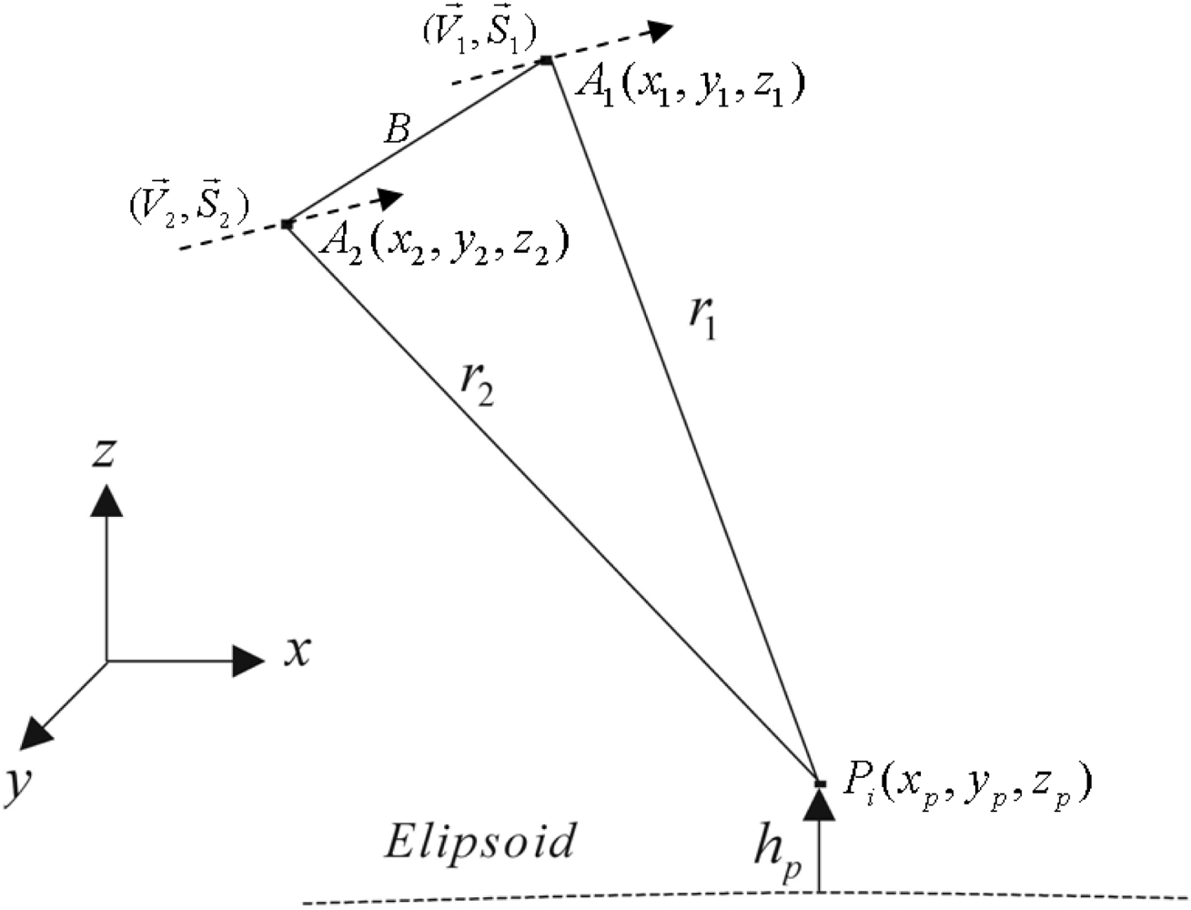
SAR Interferometry is based on the measurement of the phase difference from the complex-valued resolution elements of two co-registrated images, acquired by two separated antennas (baseline B) as shown in
Figure 1. The measured interferometric phase is wrapped in 2π, represented by
ϕm in
Figure 1. The grid of the wrapped phase values is transformed into a grid of unwrapped phase values by using a phase-unwrapping algorithm that adds to each measured phase value a constant integer multiple of 2π, represented by
ϕunw in
Figure 1.
The phase-offset value, represented by
ϕoff in
Figure 1, is a constant phase component for the whole scene that must be estimated and added to the unwrapped phase in order to obtain the absolute interferometric phase
ϕabs, from which a digital elevation model (DEM) can be generated. The phase-offset value can be positive or negative, and is sometimes greater than 2π, depending on the interferometric SAR processing strategy used.
The proposed method to estimate the phase-offset value for an InSAR airborne system is based on the following assumptions: the interferometric SAR images are generated in zero-Doppler geometry [
13], and the atmospheric effects are negligible. Considering the previous assumptions and taking antenna
A1 as the reference (
Figure 1), the following equations can be written
with p = 1 for monostatic acquisitions and p = 2 for bistatic acquisitions schemes.
Assuming a flat-earth geometry, for sake of simplicity, the terrain height can be represented by:
From the
Equations (2) and
(3), the
Equation (4) can be rewritten as
where
h is the terrain height,
H is the platform altitude and θ the look-angle for the antenna
A1.
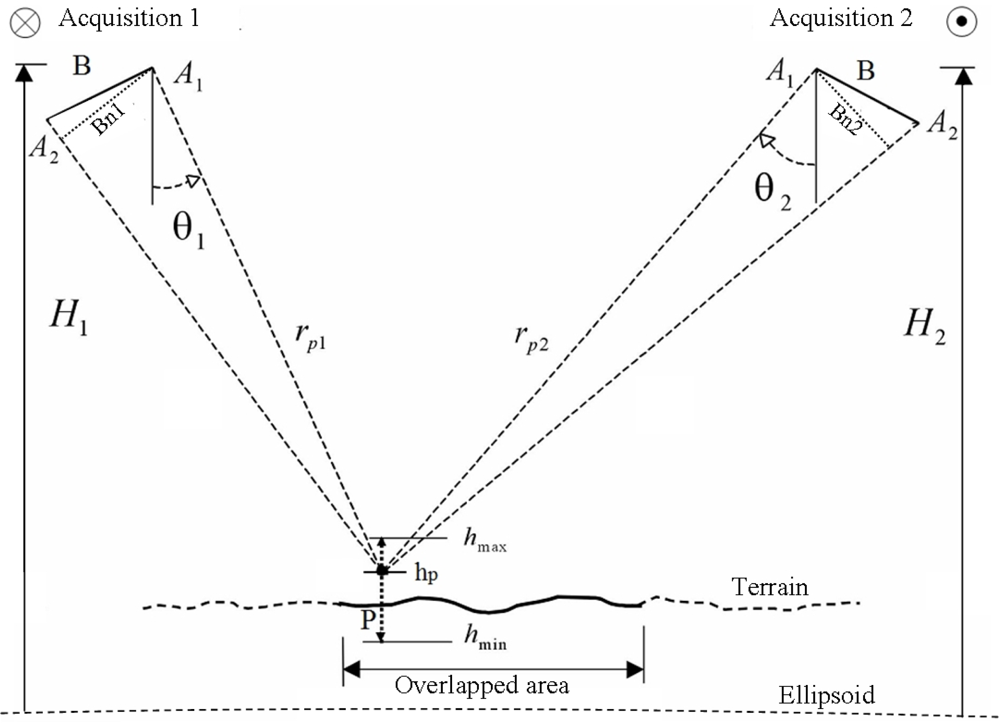
The proposed method is based on the acquisition mode shown in
Figure 2, where two InSAR acquisitions, using the same SAR configuration, are done in opposite flight directions, over a common area, which represents the usual mode for systematic mapping to diminish the shadow and layover effects. In
Figure 2, the height
hp of a point P in the overlapped area can be written, for both acquisitions, based on the
Equation (5), by:
where
ϕabs1 and
ϕabs2 are the absolute phase of the first and second acquisition, respectively.
Equation (9) shows that the absolute phases of both acquisitions, for a point P with height
hp, are only related by their incident angles. From this equation, the phase-offset
ϕoff 1 can be related as a function of
ϕoff 2, as follows:
with
Considering that Kθ and Rph are constant values at the position P with the height hp, the phase-offset value ϕoff 1 can be seen as a linear combination of ϕoff 2, depending on the relation of the incident angle and the unwrapped phase difference between the two acquisitions.
In order to build up the phase-offset function, we first consider the absolute phase value of a generic point
Pi selected, based on its geographic coordinate, with a Cartesian coordinate of (
xp,
yp,
zp) and height equal to
hp relative to an ellipsoid, as shown in
Figure 3, whose value depends on the knowledge of the slant range distances,
r1 and
r2, where for a monostatic SAR system, is given by
The slant range distances,
r1 and
r2, can be found through the Cartesian distance from
Pi(
xp,
yp,
zp) to
A1(
x1,
y1,
z1) and from
Pi(
xp,
yp,
zp) to
A2(
x2,
y2,
z2), respectively, where
A1(
x1,
y1,
z1) and
A2(
x2,
y2,
z2) represent the coordinates of the two antenna phase centers, derived from the state vector of the platform, (
V⃗, S⃗), shown in
Figure 3. The corresponding unwrapped phase value of
Pi(
xp,
yp,
zp),
ϕunwPi, in the grid of unwrapped phase
ϕunw i, can be determined by using the backward geocoding technique [
14].
The phase-offset value of
Pi(
xp,
yp,
zp), with height
hp, can be calculated by taking the difference from the absolute phase value calculated by using the slant range difference and the unwrapped phase value at this point, as follows
The phase-offset value found in
Equation (16) would be the correct one if the
Pi true height were
hp, which is the case when it uses the position and height of a corner reflector to calculate the phase-offset value. As the true height of the point
Pi is unknown, a procedure based on function that relates phase-offset to height, applied in a height interval of
hmin to
hmax (
Figure 2), was adopted to estimate the true phase-offset values for both acquisitions, assuming that the true height
hi of the point
Pi is within [
hmin,
hmax].
Attributing a height for
Pi from
hmin to
hmax in N steps, as shown in
Figure 2, and applying the same procedure discussed previously to calculate the phase-offset value for each step, one can create a set of N phase-offset values for the first acquisition. The same procedure can be applied for the second acquisition, creating another set of phase-offset values related to the same height interval. The two set of phase-offset values calculated for the point
Pi can be represented by functions, the
phase-offset functions (
POFs), as follows
where
h varies from
hmin to
hmax in N height steps.
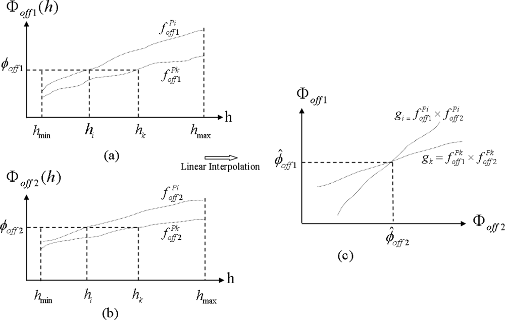
Considering that the true height
ht of the point
Pi is unknown, the phase-offset values cannot be determined from the
POFs and
. In order to overcome this problem, the following procedure was used to estimate the phase-offset values of both acquisitions:
- Firstly, as the
POFs represented by the
Equations (17) and
(18) are generated within the same height interval, [
hmin,
hmax], one can combine them creating a new function
gi, the
combined phase-offset function (
CPOF), which relates the phase-offset values in the space Φ
off 1 × Φ
off 2 for the point
Pi. A
CPOF can be represented by a function that relates the phase-offset values of both acquisitions, for each height step, through the relation based on the
Equation (13), as follows
with
The terms
Kθ and
Rph of the
Equation (19) can be considered quite constant when computed in a short height interval for the same point
Pi. Based on that, one can suppose without loss of generality, that
Equation (19) represents a linear function of Φ
ioff 1 with respect to
ioff 2, where the term
Kθ represents the angular coefficient and the term
Rph represents the constant value of this linear function. The coefficients
Kθ and
Rph change according to the range position selected for a point in the overlapped area.
- Secondly, considering another point Pk in the overlapped area, with a different range position from Pi, another two POFs, one for each acquisition, can be created for the point Pk. These two new functions can be combined, creating another CPOF, the gk, that relates the phase-offset values of both acquisition in the space Φoff 1 × Φoff 2 for the point Pk.
- Finally, as the
CPOFs gi and
gk are generated using the same height interval in different range positions, represented in the space Φ
off 1 × Φ
off 2, they have different angular coefficients, ensuring an intersection point between them, from where the phase-offset values for both acquisitions can be estimated, as illustrated in
Figure 4. The coordinates of the intersection point in Φ
off 1 × Φ
off 2, shown in
Figure 4(c), represent the estimate values of the phase-offset for the first acquisition,
ϕ̂off 1, and for the second acquisition,
ϕ̂off 2.
In order to get an accurate estimation of the phase-offset values, instead of two points, a set of points in the overlapped area, with different range positions, can be used to produce a set of CPOFs in the space Φoff 1 × Φoff, with a common intersection point. Due to noise presence in the interferometric unwrapped phase, or to abrupt variation of the phase, the common point of the intersection is not unique but has a cluster of points, very close together, from where the phase-offset values can be estimated.
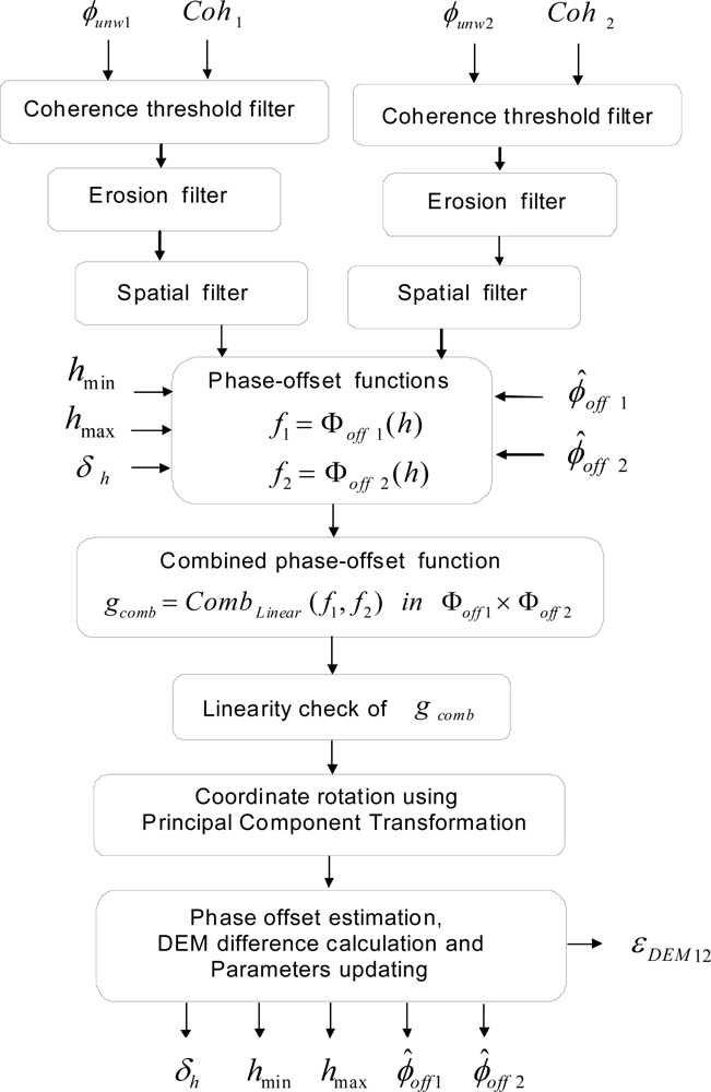
3. Processing Sequence
Figure 5 shows the processing sequence used to estimate the phase-offset values of the two overlapped acquisitions. The interferometric unwrapped phase images
ϕunw1 and
ϕunw2 are filtered in three steps. Firstly, they are filtered, based on a coherence threshold from
Coh1 and
Coh2 images, respectively, to discard points with low coherence—the threshold value is an input parameter which should be chosen according to the characteristics of the terrain and the acquisition; this filter is crucial to improve the accuracy of the estimation. Secondly, a morphological erosion filter [
15] is applied on the interferometric unwrapped phases to discard very small regions in order to decrease the disrupting effects during the
POF generation. Finally, an average filter with window size fixed according to the image resolution is used to reduce phase noise on the interferometric unwrapped phase images. To gain computation time, only boxes around the points of interest are filtered. After the filtering steps, the positions of the set of points in the overlapped area are selected to carry out the generation of the
POFs.
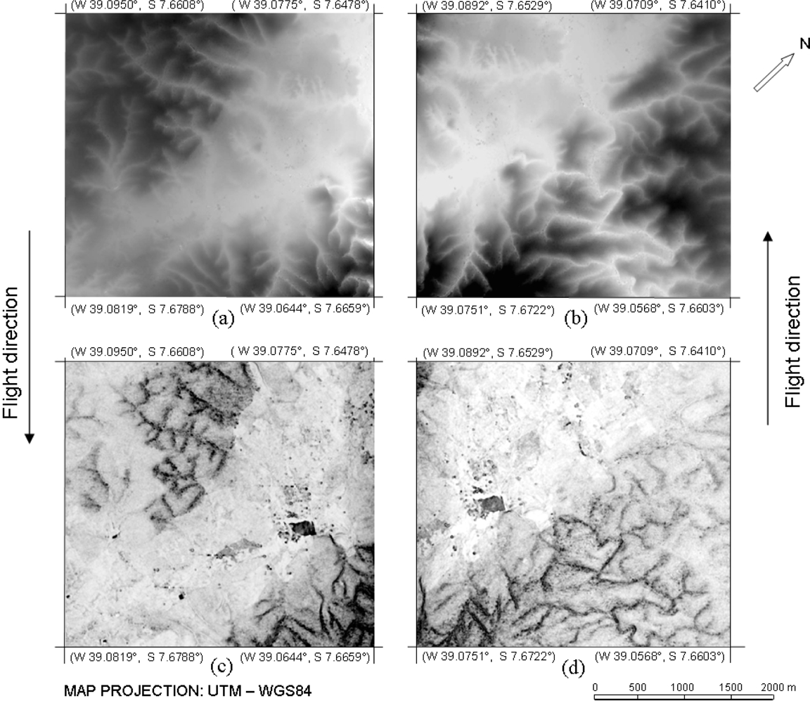
To illustrate the processing step that generates the
POFs shown in
Figure 5, a processing sequence was performed in a pair of the InSAR data gathered by the OrbiSAR-1 X-band system shown in
Figure 6. The generation of the
POFs f1 and
f2 for a selected point in the overlapped area, shown in
Figure 5, is based on the approach previously described and represented by
Equations (17) and
(18); in the next step of the processing chain, the
POFs are combined through a linear combination, creating a
CPOF gcomb in the space Φ
off 1 × Φ
off 2.
Carrying out the same operations for a set of points in the overlapped area, a set of functions
gcomb can be created from where the intersection point can be estimated.
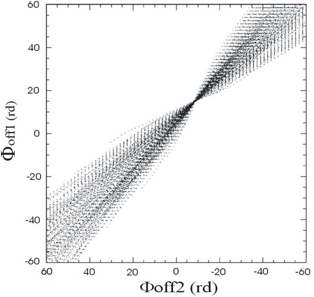
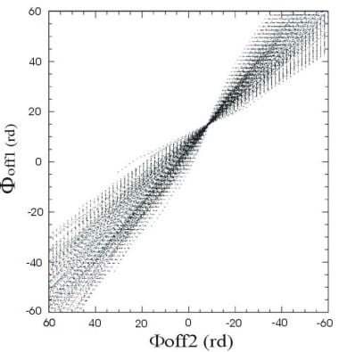
Figure 7 shows the set of
CPOF for 100 points scanned in the overlapped area in a height interval [
hmax −
hmin] equal to 200 m, based on the knowledge of the terrain topography from the SRTM DEM data, and a height step
δh equal to 2 m.
The
CPOFs have a linear behavior close to the intersection point. However, disturbing effects related to noise, terrain irregularities and the presence of range waves [
16], among others, can make the offset-functions have a non-linear behavior. To avoid the use of the disrupted functions, a filter based on the linearity of the function
gcomb (
Figure 5) was introduced. This filter performs a linear approximation of the curves and uses the chi-square goodness of fit statistics [
17] to decide which ones will be used for the estimation and which ones will be discarded.
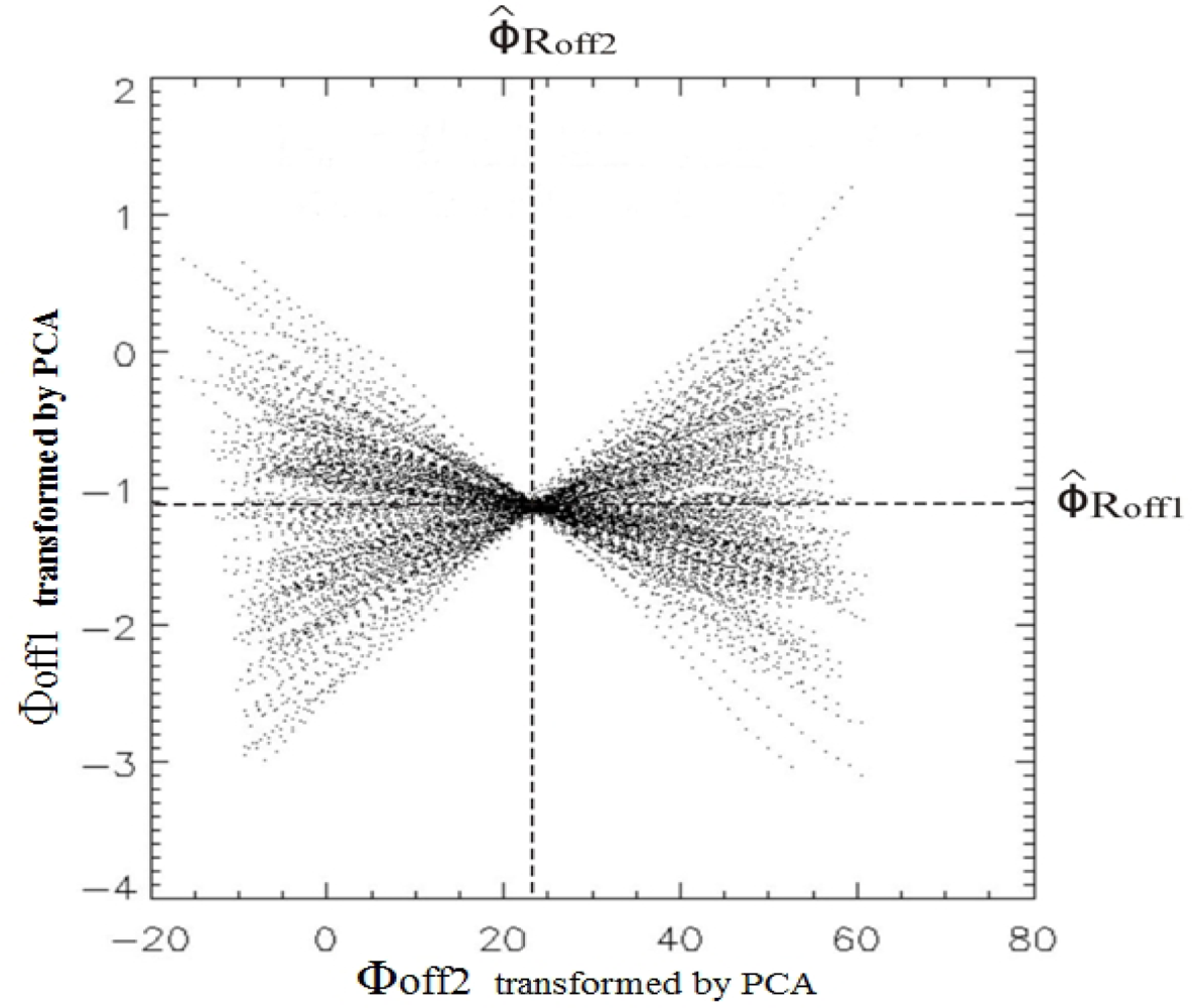
In order to make it easier to determine the intersection point of the
CPOFs, the
CPOFs are rotated using the Principal Components Analysis (PCA) [
18], which is a mathematical procedure that uses an orthogonal transformation to convert a set of observations of possibly correlated variables, in this case the set of
CPOF
s gcomb, into a set of values of uncorrelated variables called Principal Components.
Figure 8 shows the
CPOFs transformed by PCA. We can notice that PCA uncorrelates the functions, causing a spread and rotation of the
gcomb functions, allowing an easy determination of the crossing point by finding the minimum dispersion value of these transformed functions on the horizontal axis, from where the transformed phase-offset values can be determined. Finally, the transformed phase-offset values are transformed back using the Principal Components Coefficients, providing an estimation of the phase-offset values for both acquisitions,
ϕ̑
off 1 and
ϕ̑
off 2. From these estimated phase-offset values, the absolute interferometric phase for both acquisitions can be determined by using the
Equation (1).
This method works basically in two iterations. Firstly, the coarse phase-offsets values are estimated using a height interval [
hmax −
hmin] and a height step
δh, according to the knowledge of the terrain mean height from the SRTM DEM data. Secondly, the coarse phase-offsets estimated values,
ϕ̑
off 1 and
ϕ̑
off 2 (
Figure 5) are used to decrease the height interval and the height step for the second iteration to allow a fine estimation. In some cases, a third iteration can be tried to improve the estimation. For each iteration the accuracy of the phase-offset values can be evaluated through the root mean square error between the DEMs in the overlapped area,
ɛDEM12, of both acquisitions (
Figure 5), which should be very small when the phase-offset values are well estimated.
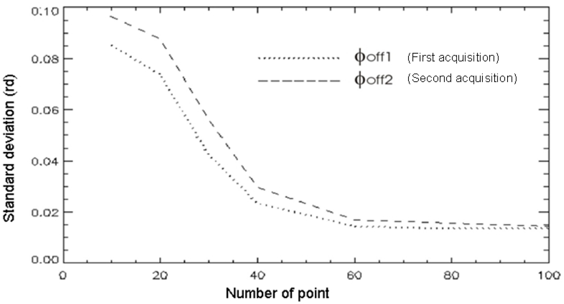
An important issue regarding the accuracy of the phase-offset estimation using the proposed method, is the number of points selected in the overlapped area used to build up the
POFs. A statistical simulation using points randomly distributed in the overlapped area showed that the phase-offset values become stable after 60 points, as shown in
Figure 9. This simulation was performed using a pair of unwrapped interferograms shown in
Figure 6, whose area is characterized by hills and vegetation, presenting a diversity of coherence values.
The performance of the proposed method regarding the size of the overlapped area in range direction was checked by changing the overlap percentage in a range direction, varying from 20% to 90% of the swath width. For each fixed percentage, the algorithm was executed ten times. For each execution, the points used by the algorithm were randomly distributed in the overlapped area within a fixed range. The phase-offset mean values and standard deviations for the X-band of the first acquisition for each fixed percentage used are shown in
Table 1.
It can be noted from
Table 1 that the performance of the method regarding the percentage used is quite robust; percentages lower than 40% and higher than 80% present a slightly larger standard deviation. We noticed that for percentages less than 30%, the incident angle diversity is low, generating the intersection of noisy
CPOFs. For percentage greater than 80% the disrupting effects in the
POFs were more pronounced due to the presence of residual undulations in far range regions of the interferograms, caused by the receiving of delayed signal components from multiple reflections [
16], thus decreasing the accuracy of the estimation. The flight configuration should be planned to ensure that the overlapped area in range direction is within the percentage interval of 40% to 80%, corresponding to an incidence angle difference between the two acquisitions of 9 to 21 degrees, ensuring an incidence angle diversity to give the necessary angular coefficient to the
POFs, allowing an easier determination of the crossing point for the estimates of the phase-offset values.
4. Results and Discussion
The presented method validation was carried out in a test site area in the south-west of Brazil, Cachoeira Paulista, São Paulo state, using data from the OrbiSAR-1 system in X- and P-bands, with the parameters shown in
Table 2. Four corner reflectors were deployed to the test site area to provide an accurate phase-offset estimation, which was used as a reference.
To evaluate the performance of the presented method, firstly, the corner reflectors were used to estimate the phase-offset values, followed by the absolute phase determination and the DEM generation for X- and P-bands. The same procedure was performed using the proposed method to estimate the phase-offset values, considering an overlapped area of approximately 60% of the swath width and a coherence threshold of 0.6 for X-band and 0.5 for P band. About 80 points randomly distributed in the overlapped area were used to build up the
POFs in this estimation. The DEMs and geocoded images were generated with a spatial resolution of 2 m.
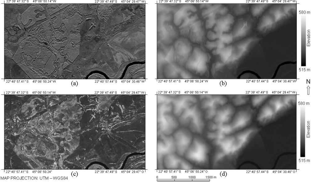
Figure 10 shows part of the geocoded images and DEMs of X-band and P-band, generated by using the phase-offset values estimated with the proposed method.
The quality of the results regarding the estimate of the phase-offset values, the first based on corner reflectors at the scene and the second based on the proposed method, are presented in
Table 3, showing that both methodologies provide quite close results. In this analysis, the phase errors induced by the temporal, baseline and volume decorrelation were not considered, since the contribution of these phase errors was embedded on the grid of unwrapped phase used in both methods.
The X-band and P-band DEMs generated with both phase-offset estimation methods were evaluated in 16 GCPs measured with GPS survey: the results are shown in
Table 4. The results in terms of mean and standard deviation are quite similar for both bands and methods used, showing that the proposed method for phase-offset estimation is a reliable automatic tool for generating accurate DEMs based on SAR interferometry.
The results shown in
Table 4 reinforce the results presented in
Table 3, where quite similar phase-offset values found with the two methods collaborate to generate quite similar DEMs. It can be noted from
Table 4 that despite the fact that corner reflectors can provide the best phase-offset estimation, the DEMs from X- and P-band present errors when compared to GCPs. That could be explained from phase error mentioned before, which is not evaluated in the present work. In
Table 4 we also notice that the mean difference and the standard deviation regarding the 16 GCPs for X-band are greater than those for P-band; this can be explained by the fact that the DEM generation process is more affected in vegetated areas, which is more pronounced for X-band data due to its low penetration into the vegetation.
4.1. Error Analysis
The height derived from the interferometric phase is very sensitive to phase errors. According to [
19], the height error is related to phase error by:
where
σϕu is the phase uncertainty,
Bn is the normal baseline,
θ the incident angle,
r the slant range distance and
λ the wavelength.
The standard phase error and the phase uncertainty with 95% of confidence level, according to [
17], are given respectively by:
and
where
σϕ is the standard deviation of the interferometric phase, N is the number of measurement and
μϕ is the mean phase error.
Table 5 shows the height error regarding the phase-offset estimation difference between the two methods, with corner reflectors and with the presented method, shown in
Table 3, considering that the estimation using the previous method leads to the best estimation. Taking into account only the phase-offset estimation error of this proposed method, leads to a height uncertainty of around 0.5 m for X-band and 1.1 m for P-band, with a 95% confidence level, as shown in the last row of
Table 5 for the test carried out in Cachoeira Paulista.
4.2. Test Result without Using Corner Reflectors
The advantage of not using corner reflectors (GCPs) to estimate the phase-offset values on forested areas is tremendous. Dispensing the reflectors can lead not only to lower costs but it can also diminish the environmental impact associated with corner reflector deployment. In certain regions, like the dense Amazon forest or in fluvial regions, access to appropriate areas to deploy the reflectors can be difficult. Based on that, a test was performed in the Amazon rainforest area characterized by quite flat relief, without the use of corner reflectors. Several tracks were flown so that they crossed each other to compute the DEM difference in the intersection areas. The data were acquired with the same characteristics shown in
Table 2. The phase-offset values were estimated using an overlapped area of approximately 50% of the swath width, where about 100 points randomly distributed in this overlapped area were used to build up the
POFs for the phase-offset estimations. The coherence threshold used to select points was 0.6 for X-band and 0.5 for P-band. The DEM of X-band and P-band were generated with a spatial resolution of 2.5 m. The goal of this test was to verify if the phase-offset values would be well estimated for each track, enabling the generation of quite similar DEMs on the intersection areas.
Figure 11 shows the X-band DEMs of the tracks in color scale.
Table 6 shows the computed statistics between the DEMs for X-band and P-band in the intersection areas of all tracks. It can be noted from
Table 6 that the mean value differences are small for both bands, while the standard deviations have significant values, caused mainly by the high variation in the DEMs due to the forest structure, aggravated by the different looking angles in the intersection areas; this is more pronounced for X-band due to its low penetration into the forest, which makes it more susceptible to canopy variation. The standard deviations of the slope in range and azimuth directions were quite small for both bands. The estimates of height uncertainty at the 95% confidence level were around 3 m for both bands. In this computed statistics, all phase errors that contribute to lower the accuracy of DEMs were taken into account.
5. Conclusions
The method for phase-offset estimation, based on phase-offset functions presented in this work, has good potential for operational application, as it does not require the presence of GCP or a priori information, and at the same time is able to provide the accuracy requested for DEM generation.
The results presented in
Table 3 and
Table 4 using OrbiSAR-1 data show that the estimation of the phase-offset values generated quite similar results to those produced through the use of the corner reflectors, for X-band and P-band, indicating that the phase-offset estimation can be automatically done, leading to a lower cost and a faster estimation. Taking into account only the phase-offset estimation error, shown in
Table 3, the height uncertainty regarding this error, shown in
Table 5, indicates that the generation of X-band and P-band DEMs could be carried out in the scale of up to 1:5,000 m, according to [
20].
The potential for mapping rainforest area was checked and the results are presented in
Table 6, indicating that the proposed method can provide reliable phase-offset estimation to generate X-band and P-band DEMs in the scale of up to 1:12,000 m, with a vertical accuracy at the 95% confidence level equal to 2.768 m for X-band and 2.904 m for P-band.
The results presented in
Tables 5 and
6 show that P-band has a somewhat larger height uncertainty than X-band, caused probably by the different scatter center positions of the pixels for the two acquisitions, since the penetration of the microwaves in the vegetation changes according to the incidence angle, which is more pronounced for P-band, increasing the error in estimating the sphase-offset values.


