Article

Detecting Mountain Peaks and Delineating Their Shapes Using Digital Elevation Models, Remote Sensing and Geographic Information Systems Using Autometric Methodological Procedures

1
Faculty of Civil and Geodetic Engineering, University of Ljubljana, Jamova 2, SI-1000 Ljubljana,Slovenia
2
Scientific Research Centre of the Slovenian Academy for Sciences and Arts, Novi trg 2, SI-1000 Ljubljana, Slovenia
Remote Sens. 2012, 4(3), 784-809; https://doi.org/10.3390/rs4030784
Submission received: 16 December 2011 / Revised: 2 February 2012 / Accepted: 2 February 2012 / Published: 21 March 2012
(This article belongs to the Special Issue 100 Years ISPRS - Advancing Remote Sensing Science)

Abstract

:
The detection of peaks (summits) as the upper parts of mountains and the delineation of their shape is commonly confirmed by inspections carried out by mountaineers. In this study the complex task of peak detection and shape delineation is solved by autometric methodological procedures, more precisely, by developing relatively simple but innovative image-processing and spatial-analysis techniques (e.g., developing inventive variables using an annular moving window) in remote sensing and GIS domains. The techniques have been integrated into automated morphometric methodological procedures. The concepts of peaks and their shapes (sharp, blunt, oblong, circular and conical) were parameterized based on topographic and morphologic criteria. A geomorphologically high quality DEM was used as a fundamental dataset. The results, detected peaks with delineated shapes, have been integratively enriched with numerous independent datasets (e.g., with triangulated spot heights) and information (e.g., etymological information), and mountaineering criteria have been implemented to improve the judgments. This holistic approach has proved the applicability of both highly standardized and universal parameters for the geomorphologically diverse Kamnik Alps case study area. Possible applications of this research are numerous, e.g., a comprehensive quality control of DEM or significantly improved models for the spatial planning proposes.

Graphical Abstract

1. Introduction

The aim of this study is the detection of mountain (called also topographic) peak points and the analysis of their surroundings in order to determine their shape. Automated morphometric techniques and procedures are required to solve this complex task. The methods developed are intended to be studied holistically according to a number of other points of view in the context of spatial studies, in order to arrive at a reliable conception of a peak. The following three associated introductory challenges are relevant here:
  • semantics, definitions, conception and standardizations
  • appropriate data sources
  • morphometric algorithms based on a digital elevation model (DEM)

1.1. Semantics, Definitions, Conception and Standardizations

A landform peak can be defined as a point higher in elevation than the adjacent area. The shape is a geometric property of the peak point on an arbitrarily selected surrounding area (depending on the scale or level of detail) that is morphologically expressed as being sharp, blunt, oblong, circular, conical, or other. Both definitions are vague and subject to further discussion.
Professional mountaineers have perhaps the best knowledge of the peaks and other characteristics of the mountains from different regions worldwide, but it partly depends on their subjective perception and experiences. Researchers have been trying to measure and standardize mountain peaks for at least the past 120 years [16]. Defining a peak is a conceptual problem that requires a certain level of abstraction which is an essential part of the model, and which should have subsequent feasibility for the applicable automation process. The concept of a peak is contextually associated with several other concepts, such as the concept of the whole mountain, its roughness, locations of prominence and others, all of which are important for an enriched understanding of the problem in question. Size and shape (in context) are important criteria for the definition of peaks as a landform category or even for the construction of the landform taxonomy [7]. Until now, definitions of peaks have been based mostly on tradition, experience and visual appreciations—on a subjective perception of the natural appearance of the peaks [1]. The different views of the problem studied in this research can serve as sources of a comprehensive definition of a mountain peak, which can be further used as a source for an enhanced ontology of mountain peaks.
The concepts and definitions of the term “peak” must be considered in association with the wider topography (regional and global) and its relation to the term “mountain”, considering the entire mountain or range. The concept of a peak as a topographic and morphologic extreme in a specific geographical space has several other meanings in a semantic sense. However, our aim here is not to find absolute definitions, but merely to discuss the complexity of the subject of our study.
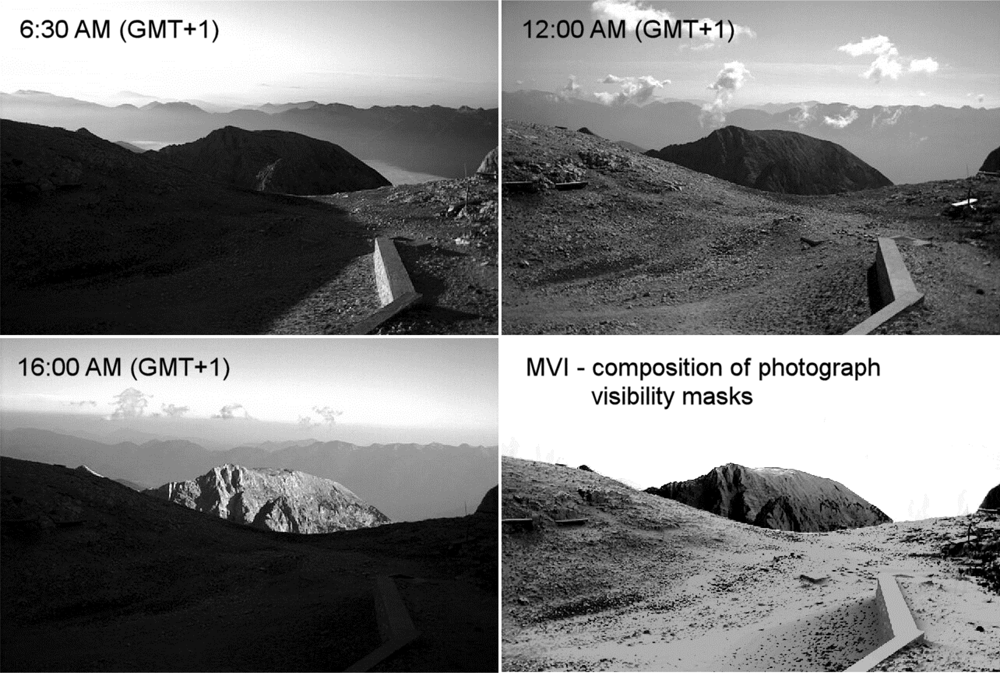
Just as the most significant peaks are visible from a distance, in the immediate neighborhood the peaks on the lower rising ground are also visible. The peaks may appear different when viewed from various distances (e.g., the peak appears oblong from 100 m, but circular from 1 km), from different directions—oblique or vertical views (e.g., sharp from one valley and blunt from another), when view at different times of the day (Figure 1), and also in different weather conditions (including the visibility phenomenon) with different snow cover or during different seasons. Furthermore, peaks are conceived in different ways worldwide, which impacts on the terminology. For instance, the characteristics of the Alps, Carpathians, Himalayas or even the Pannonian Plain are quite distinctive. These factors depend on physical and environmental properties, such as the elevation above sea level, geological properties, the shapes of peaks, the illumination (Figure 1), vegetation, and on the particular perception of an individual observer. These findings may lead to mentally various perceptions and consequently to different identification, conceptualization and classification by the observer. In order to provide a proper description of the peaks, the landscape in question and its properties has to be considered.
The relation of the peak to the roughness concept of the relief refers to the irregularity of a terrain, which may even be defined with self-similar fractals. The terrain roughness is geomorphometrically related to the periodic functions, where a texture is used to refer to the shortest wavelength in topography, and the grain used to refer to the longest significant wavelength [
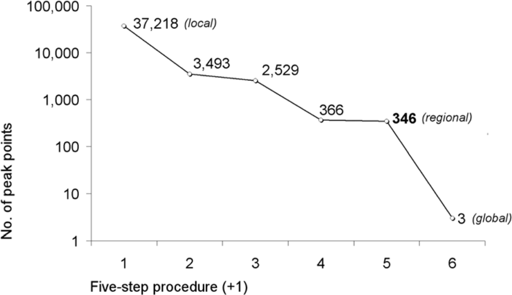
5]. Three types of peaks will be discussed according to their different size-scale (and level of detail): local, regional and global. The local peaks represent significant maximum points of the texture, while the regional and global peaks are related to the grain. The concept of roughness raises the many further complexities of the peaks e.g., the relation to aesthetic quantification.
Within common concepts, the peak is defined as being any point on a surface that is elevated by a certain difference in height with respect to its surroundings. A peak must be autonomous in the sense of possessing individuality, interest and other characteristics. The peaks might be considered in addition to the features that satisfy the especially subjective criterion of a “well defined morphology”. These primary criteria are referred to as topographic, morphologic and mountaineering [2].
According to dictionary definitions, standards, and encyclopedias, e.g., [7,9,10], the term peak is less technically defined, i.e., mostly with reference to the morphologic properties of the surface that surrounds the higher point. These definitions may therefore be vastly dissimilar. Possible peak definitions are: “any rising ground that splits the mountain in its higher part”; “upper, usually folded part of the mountain”; “the highest point of the mountain”; “the point on a surface that is higher in elevation than all points immediately adjacent to it”. More precise definitions of this phenomenon concern size and shape and distinguish between the terms “peak” and “summit”. The summit means the highest elevation on a profile, whilst the concept of a peak depicts part of a summit with moderate to very steep sides [11]. However, this last definition already reflects a corresponding ontology and cultural semantic aspects (e.g., concepts are not the same in English and the Slovenian language) [1,12]. The term “peak” is used in the study to correspond to a point.
The concepts of regional and global peaks should also be discussed. Regional peaks are complex features which occur in the most common definitions of peaks that are found in basic dictionaries, described by the UIAA, and defined by people who live in the mountains. This term is defined by a broader range of topographic, morphologic and other so-called mountaineering properties on a regional scale [2]. Global peaks are a subset of regional peaks. Global peaks are limited to the most prominent or salient peaks of a given mountain (range), e.g., the entire Kamnik Alps. Global peaks have acquired cultural importance and have been of immense interest to humans over centuries or millennia. Therefore, they are defined according to the mountain range and/or according to their prominent location.
Peaks are also defined by referencing topographically related mountain ranges (i.e., groups of mountains), mountains, massifs, hills, or hill-like features [7]. Similarly, the terms “mountain” and “hill” also vary in definition worldwide. Thus, only the term “mountain” is discussed here in order to support its wider geo-connoted conception. The concept of a mountain is more complicated and subjective than the concept of a peak, and it involves aesthetical, ecological, chronological, and other factors. The term mountain is not a real physical (bona fide) object. It can even be interpreted as a fiat object, which only exists in the human understanding and division of the landscape [1215]. However, it is clear that mountains exist as real correlations of everyday human thought and action, and that they form the archetype for geographic objects [12].
A mountain can be defined as a natural rise in the Earth's surface that usually has a peak (or a summit) [8]. Similarly, the term mountain is defined as a landform that sufficiently extends above the surrounding terrain over a limited area with comparatively steep sides and a peak. A peak (a highest point or a highest ridge) and the mountainside (part of a mountain between the peak and the foot) are considered to be the main sections of a mountain [16].
The mountain as an object comprises the following morphometrical parameters: size, perimeter length, maximum elevation, slope, mean or average slope, slope gradient, relative or local relief, relative massiveness (according to stage of erosion), shape, roughness, texture and grain, etc. [5,17,18]. The following are those definitions that contain quantitative operational definitions: mountains are usually steeper and taller than hills; they are often considered to be hills that rise over 600 m (a.s.l.) in height; another study utilizes the higher vegetation zones as the important criterion for defining it as a mountain [4]; a mountain is defined with an altitude (height), slope and relative height distinction; the lowest limit is 300 m in the altitudes of 65°N and 55°S and up to 1,000 m at the equator. A team of Kapos [19] used criteria based on altitude and slope in combination with a depiction of the world’s mountain environments to form their definition. They proposed seven classes based on slope and local elevation range. The most important for the definition of a mountain are: (classes 1 to 3) elevations >2,500 m; (class 4) elevations 1,500 to 2,500 m and slope ≥2°; (class 5) elevations 1,000 to 1,500 m and slope ≥ 5° or local elevation range >300 m (radius of 7 km); and (class 6) elevations 300 to 1,000 m and local elevation range >300 m outside 23°N to 19°S (radius of 7 km).

1.2. Appropriate Data Sources

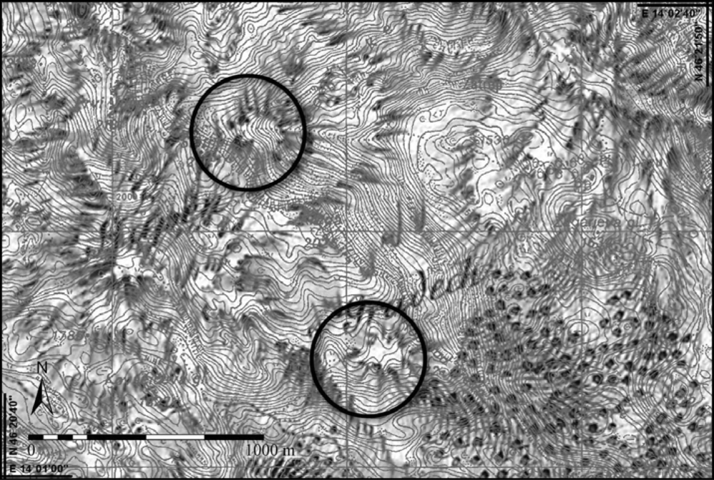
The mapping of peaks and mountains has generally been performed manually through fieldwork and the visual interpretation of topographic maps, aerial photographs and satellite images. An example (Figure 2) presents an old Josephine military topography (scale 1:28,800) from the end of 18th century that was verified with an overlaid modern topographic map demonstrating that the peak positions are in this case considered to be correct (scale 1:25,000, DTK 25). On the old map, some peaks are clearly detected but with their positions have been incorrectly mapped. One of the reasons for this is that some peaks had not been climbed yet when this old map was produced.
The problem of the remote sensing techniques that use aerial photographs and satellite images, from which modern maps are produced, is that a large amount of semantic information is inherently hidden in these data sources. Moreover, the detection and interpretation of topographic peaks is problematic in forest areas.
Another potential data source for studying topographic peaks is a digital elevation model—DEM (or digital terrain model—DTM). The DEM allows a very high level of automation for the study of geomorphologic features [20]. Its geomorphological quality and appropriate (high) scale/resolution (Table 1) are crucial for successful applications [21,22]. However, the lack of both properties is a distinctive problem for real data sources application. Typical sources of the DEM are maps, aerial photographs and satellite images, as mentioned before, which is not encouraged. Fortunately, more independent and higher quality data sources are available nowadays based on LIDAR or SAR technologies as important remote sensing techniques for topographic data collection.
A geomorphologically higher quality DEM would be required in order to study the peaks of flatter areas, compared to the requirements in the hilly areas, such as the Pannonian Plain. The resolution of the DEM controls an optimal scale and the level of detail of the peak determination, particularly local peaks. It should reflect the discussed topographically-relevant terrain roughness. The integrative study of more alternative datasets (and techniques) in a geographical information systems (GIS) environment can improve the judgments in morphologically enhanced studies [22].

1.3. Morphometric Algorithms Based on a Digital Elevation Model (DEM)

The extraction techniques of peaks have evolved considerably—from manual in the past, through computer assisted, to various automated methods over the last decades. The automated application of the detection of peaks and the delineation of their shape is discussed through morphometric algorithms based on a geomorphologically accurate DEM. The algorithms for local peak detection are considered as an ordinary problem, while the algorithms for topographic (regional and global) peak detection demand more complex solutions to the problem of feature extraction and recognition, all based on morphometric image processing or spatial analysis techniques.
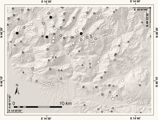
Local peaks are computed using the most elementary numerical (computer-based) peak detection approach from the DEM. The algorithms are based on an assessment of local extremes, e.g., the Peucker and Douglas method [23] that detects every rise in ground elevation. The problem can be resolved with tools as part of both: standard remote sensing (image processing) and GIS (spatial analysis).
The existing solutions for the numerical implementation of regional peaks incorporate mostly only topographic criteria, e.g., an algorithm to extract the number of peaks based on a morphological smoothing method [24], and an algorithm based on the minimum drop surrounding peak criterion [29].
The procedures for global peak detection use a considerably larger surrounding area than the procedures for regional peak detection. Their definition is either related to (A) the entire mountain range, or (B) a prominent location.
(A) Most of the developed automated techniques concentrate on the detection or classification of whole mountains or mountain ranges, e.g., the algorithms for feature-matching [3], the component-labeling algorithm applied to the mountain terrain class [17], a local histograms analysis [25], and mathematical-morphological based algorithms [16].
(B) A number of studies have attempted to establish prominent locations (peaks) using numerical algorithms. Their characteristic technique is to study specifically cultural responses that influence human behavior, including beliefs, taboos, and rituals, etc. Prominent peaks are explored by analyzing their properties according to their wider surroundings. This includes: an exposure index, cumulative viewsheds, defining location hierarchies (nested peaks), taking into account the fuzziness of general multi-scale landscape morphometry, a comparative evaluation according to a multi-scale prototypicality of peaks identified, a computation of horizon lines based on a viewshed analysis, and the identification of the salient points on the horizon based on a hierarchical decomposition of the projected horizon, etc. [14,2630]. A comparison of the automated implementation of local, regional and global peaks can be seen in Table 1.
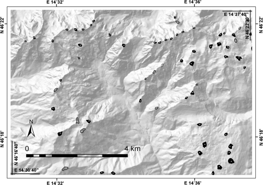
The comprehensive peak detection procedure should also consider the morphological shape of peaks. The topographic shape delineation of a peak is a more complex conceptual and implementational problem than its detection. The algorithms that touch on the problem of shape analysis relate to the issue of peak prominence discussed in the previous paragraph. The automated shape analysis procedures can additionally improve the strategy for detecting peaks.

2. The Problem

Considering the challenges introduced, the technical description of a regional peak has been established according to the rules of the International Mountaineering and Climbing Federation (UIAA) [2]. The rules of the UIAA are formulated for those peaks higher than 4,000 m in the Alps according to the following three criteria: topographic, morphologic and mountaineering (alpine). While the mountaineering criterion is the most subjective and qualitative, the topographic and morphologic criteria have a certain potential to be processed by quantitative automated procedures. All criteria together can be considered as a qualitative peak analysis and reasoning [31].

2.1. The Concept of Regional Peak Parameterization

The topographic criterion defines the level of height difference between each peak, and specifies that the highest adjacent pass or notch should be at least 30 m (calculated as an average of the peaks at the limit of acceptability). An additional criterion can be the horizontal distance between a peak and the base of another adjacent peak [2]. The suggested application of this rule is by a geometric analysis on the DEM: the main criterion being a definition of the relative height (dH) of the potential peak that should be split by the adjacent peaks with a certain gap (which should be 30 m lower than the peak). An additional criterion is defined as the minimum horizontal distance (dL) between the peaks, which is related to peak density [5], which in turn is related to grain as part of the roughness concept. These values help to define the dominance of the potential peak. The larger the measured values, the more extensive and significant the peak becomes.
The morphologic criterion takes into account the overall morphology and aspect of the peak, especially when applied to shoulders, secondary peaks, rocky outcrops, etc. [2]. The proposed application focuses various techniques of spatial analysis for determining the various sizes of the immediate peak neighborhood (determination of mountain area Gp, potential surfaces Pij, see Table 2 for appropriate indexes). The shape of the upper part of the mountain is therefore considered, and much depends upon its geological characteristics.
The following mountaineering criterion takes into account the importance of the peak from the viewpoint of mountaineers: the quality of the routes that lead to the peak, the historical significance of the peak, and the frequency it has been climbed [2]. This criterion is the weakest and most difficult for standardization and numerical application. It considers the inspection of terrain as a subjective human perception. With the evolution of mountaineering, the criterion may change in the future. The mountaineering criteria are not intended for parameterization; they are simply used as means of verifying and interpreting the results.

2.2. The Concept of Peak Shape Parameterization

The morphologic criterion of the regional peak is studied in greater detail. Morphological shape of the peak can be explained through typical categories of sharp, blunt, oblong, circular, conical shapes, etc. The shape categorization is a complex semantic and conceptual problem that may be used to support the peak definition. The definition of the shape might be developed on different levels.
In this study, a two-digit numeric code system is proposed. Category i explains the properties of scale/size of the peak, whilst category j describes the (dimensionless) shape of the peak. Thus, this code system relates the determination of the peak to the shape delineation problem. For example, an oblong regional peak is, according to Table 2, assigned the number 23, which is a composition of category i and category j to ij.
The characteristics of the shape of a peak are dependent on each other and are not universal. Table 3 shows the linkages between the shapes (category j; Table 2) that are applicable in the shape delineation modeling. For example, the most complex, conical shape should include sharp and circular shapes (black backgrounds of field), and should exclude blunt and oblong shapes (white backgrounds).
Additional morphological shape categories might be studied beyond those that are listed in the peak taxonomy of Tables 2 and 3 (e.g., a pyramidal peak). The category of shape featured in Table 2 may be further (sub)classified and additionally coded to categories that describe the xy ratio (2D footprint or floor plan, e.g., eccentricity or orientation) and the vertical to horizontal ratio (cross section, e.g., slope or concave/convex) parameters of the shape of a peak.

3. Methodology

No single criteria or parameter can be used to determine the complex different terrain forms. A combination of significant parameters can increase the reliability of terrain measurements [11]. Two procedures are proposed. The first has been developed to detect the points of topographic (regional and partly global) peaks. Topographic and some morphologic criteria based on the UIAA directive [2] are employed using a numerical procedure and algorithms, while selected mountaineering criteria are used for their verification and interpretation. The second procedure has been developed to analyze the surrounding area in order to determine their shapes. The morphologic criteria are realized according to algorithms that use classified peak shapes.
The methodology of both interconnected procedures is considered to be part of the specific (in contrast to general) (geo)morphometry that applies to and describes discrete landforms such as peaks or talus cones and can involve arbitrary decision-making in the quantification of its concepts [5,32]. The expectation for this methodology is that it demonstrates a certain potential for bridging qualitative peak concepts and terminology to achieve more quantitative definitions of geographically delineated peaks.

3.1. The Detection of Peaks by Topographic and Morphologic Criteria

The following five-step procedure is based on the classification and extraction algorithms for fulfilling the basic topographic and morphologic criteria for detecting regional peaks:
  • the calculation of local peaks as a local maximum in elevation [23]
  • the selection of peaks that are morphologically not on flat areas (peaks on plains are denoted as Gp)
  • a further selection process considering a minimum horizontal distance (dL) between peaks
  • a further selection process considering a relative elevation (dH) of peaks
  • a final selection of the regional peak points considering the potential surfaces of peaks (Pij, see Table 2 for indexes)
In each step of the procedure only those peaks are processed which satisfy all conditions in previous steps. Thus, in every new iteration a smaller subset of peaks is generated. The procedure for the detection of regional peaks (and global in the additional sixth step) within the five-step procedure is presented in Figure 3. The steps are described below in greater detail.
  • In the first step the local peaks are calculated by applying a local moving window with the kernel of size 3 × 3 cells, dedicated to raster-based spatial data analysis, e.g., [33]. This step is based on topographic criteria.
  • All of the local peaks on the flat areas (Gp) are eliminated setting criteria NOT Gp. The removed local peaks are part of insignificantly convex areas. The classification of Gp is part of a landform regionalization process applied to plains, low hills, hills, and mountains. This process applies a combination of slope, curvature and elevation of terrain [22]. With an additional threshold those peaks which do not surpass a certain absolute minimum elevation (e.g., <600 m) can be eliminated. This step employs morphologic criteria in order to optimize the procedure significantly.
  • The minimum horizontal distance (dL) is applied. Only those peaks which represent the highest within the circle of radius dL are retained. The adjacent peaks are therefore arbitrarily removed with dL > [150 m, 200 m]. This step is based on the topographic criteria and follows the grain concept.
  • The analysis of the relative height of the peaks (dH) serves as a basic topographic criterion. The algorithm determines the areas around the individual peaks that register as being up to the dH lower than the corresponding peaks. Next, the entire area is examined and the other peaks that were identified in the third step are counted. If no peak has been identified, then the examined peak is adopted. Starting with the highest peak, the procedure is repeated until the lowest peak has been processed. The peaks eliminated in the previous iterations of this procedure are not further examined. The condition for their removal is set to dH > [25 m, 30 m]. There are further options to calculate the results, e.g., with contour lines in vector form [11,34] or by filling the pits of the inverse DEM in raster form.
  • The final step is based on the morphologic criteria. A continuous potential surface of regional peaks of any shape (P29) is applied (see Table 2 and the final step of the six-step procedure in the following section). The appropriate threshold setting for P29 determines the elimination of several peaks on morphologically less rough areas. The progressive elimination of peak points can be applied with a continual increase in the surface threshold. The remaining points are finally adopted as regional peaks with respect to the topographic and morphologic criteria.
The five-step procedure runs twice by applying two slightly different parameters in steps 3 and 4. In the first execution the parameters are set to dL = 200 m and dH = 30 m, and in the second to dL = 150 m and dH = 25 m. These two calculations yield slightly different but complementary results and the minima of peak points of both are considered. The global peaks are derived using the same procedure (Table 2 and Figure 3/6). In this case, the parameter dL in step 3 is arbitrarily set to 2,000 m, and a potential surface of global peaks (P15) is applied in step 5.

3.2. The Delineation of Peak Shapes by Morphologic Criteria

The application of the morphologic criterion allows for the delineation of peak shapes. However, some of the potential surfaces can also be used for a more advanced detection of peaks that has been primarily determined by various topographic criteria (see step five in the previous section). The shape analysis requires a database of peaks, in our case due to the peak detection section. The following six-step procedure is proposed as a means of obtaining a shape analysis of peaks:
  • generating the variables through the operations of spatial analysis based on the raster format
  • relating the variables with two-digit codes ij (see Table 2)
  • converting the variables into binary indexes (Ik)
  • the further selection of the significant (descriptive) Ik
  • combining the Ik to generate a continuous potential surfaces (Pij)
  • assigning the values of the Pij to the points of peaks (determined in the five-step procedure)
The steps are described below in greater detail.
  • The standard and more innovatively composed variables are generated in this initial step. Specific spatial patterns related to the shape of peaks may be discovered in these variables. The variables are generated through a raster-based spatial analysis, as provided by GIS-tools. The basic variables are slope and curvature [21,35]. The standard variables that are based on both, a local moving window [21] of different sizes or on a local annular moving window (AMW) are: the minimum (MIN); the maximum (MAX); the mean (M); the standard deviation (STD); and the range (R; values from-to). The following innovative variables have been derived (see Table 4, Variable):
    • - the “relief above” (RA = [MAX − (value at local window center)])
    • - the “relief below” (RB = [(value at focal center)-MIN])
    • - the “ridge-drainage” (RD = [MAX+MIN-2*(value at local window center)] = RA-RB)
    • - the “rim” (RI = [MAX+MIN-2M])
    • - the “concave-convex” (CC = [(value at local window center)-M]) (as a kind of relative or local relief [5])
    One of the most applicable variables that was developed is a relative relief based on a “multidirectional visibility index” (MVI). It is based on a visibility masks calculation with regard to the variations in azimuths and zenith angles [8]. The catchment analysis (CA) is based on a calculation of cost surfaces around the peaks.
    The variables are generated using DEMs of different resolutions and differently smoothed surfaces (see Table 4, Scale).
  • Each variable is related to a single or multiple two-digit codes ij to determine the peak’s size and shape (12 possible codes) according to Table 2. Each variable can therefore be related to more peak categories (see Table 4, Code (ij)).
  • The variables as continuous functions are converted into binary (0/1) indexes I1, I2Ik by applying appropriate thresholds. One variable can be converted into more indexes (Figure 4). The threshold classification of variables to their Boolean forms Ik is determined by the following primary rule: variables are sought that have values which characterize those areas that are least likely to reflect the target property (according to codes ij); however, they should simultaneously exclude as extensive a portion of the area as possible, using the upper limits that allow all pixels of the target Ik to be retained. It is expected that the individual index Ik should cover the target areas in their entirety. The settings of the threshold parameters may be derived through various approaches or combinations (e.g., fitting the Ik areas according to a histogram analysis involving a certain portions of area, or to a certain number of detected/known peaks) based on iterative adjustment. In our case, the thresholds of every index Ik are adjusted on the basis of a few preliminary selected typical peaks (according to codes ij), derived from the five-step procedure. Nevertheless, the quality of such results depends greatly on the operator’s experiences.
  • The indexes Ik are further selected through independence and significance tests, if necessary. These tests can be processed using different statistical approaches (e.g., through regression analysis). In our case the Ik are visually assessed by (a) comparing all sets of Ik that reflect the same codes ij in order to recognize their independence, and by (b) assessing the portion of the whole area coverage to recognize their significance. Smaller portions reflect a higher level of significance. From among the many indexes, k = 35 are selected as significant (see Table 4, Index). However, the independence and significance of the indexes Ik do not greatly influence the result of this procedure, but rather decrease the number of indexes Ik.
  • The aim of this step is to combine more Ik in order to generate continuous potential surfaces (Pij) (see Figure 4). The combinations of the Ik can be preceded by fundamental analytical operations, such as Boolean algebra, and arithmetical and relational operations [36]. In our case, we have applied a so-called graphical approach to our model which is based on the Boolean algebra of the indexes Ik, which have been proved in some way to influence the location patterns of the target peaks ij. A simple sum of the indexes Ik equally determines the location potential of the response data (final model), where the expected range is a number of the total included indexes Ik. Figure 5 presents a potential surface for the determination of global peaks independent of the shape, with code ij = 19 (P19) that comprises the following indexes: I1, I14–17, (optionally additionally included, but were not: I20, I24–27, I29 as surfaces) (Table 4). The linkages between the shapes of Pij (category j; Table 2) are presented in Table 3.
  • In the final step the values of the Pij surface are assigned to the points of peaks determined in the five-step procedure. The grater is the value of the Pij in the surrounding of the particular peak, the higher is its significance (and potential). Additionally, an appropriate threshold can be applied to Pij to assign a binary decision significance/non-significance to the particular peaks. Figure 4 schematically illustrates this procedure.
There are alternative methods of analyzing the shape of peaks using the DEM (Table 4). We will consider two alternatives involving just the first step of the six-step procedure. These are based on the AMW technique and the CA variable.
The applications of the AMW are suitable for the detection of conical peaks (codes 15, 25 and consequently 14, 24; Table 2, and 1st figure in Section 4.3). An independent procedure in two steps is proposed: (a) The AMW is defined by two radii (the inner r1 and the outer r2) measured in the number of cells along the x- (=row) and y-direction (=column) of the matrix. Since the grid spacing is usually specified in real world units, the radii of the AMW may also be expressed in meters or in any other standard unit (Table 5). All cells located within the ring defined by these two radii are included in the calculation. (This step generates a continuous variable that might be used through the six-step procedure for the conical peaks delineation). (b) The results are measured in the second part of this procedure. The annular-shaped ring (ASR) is constructed with the same dimensions as the AMW used in step (a). It is centred on the points of the peaks. The average values of the variables (MIN, MAX, MEAN) are calculated for the ASR and assigned to the points of the peaks. These values are then compared to the values of the variables on the points of the peaks or compared to the heights of the peaks. The most significant results are calculated with the variable MAX.
The second approach is based on the CA, particularly on cost surfaces [2]. The cost surfaces are computed using the points of the peaks, where the slope is assigned as a cost. Therefore, this procedure may not be used in the six-step procedure. A geometric analysis of the shapes and sizes of the areas generated around the peaks in certain cost distances indicates the shapes of the peaks, especially the oblongness and the sharpness (Figure 6). The cost surfaces can be calculated to different scales using the DEMs of various resolutions. Utilizing different scales, the general shape of the whole mountain range can be assessed hierarchically starting with the small areas around the peaks and increasing to the areas at the foot of the mountains [29].

4. Results and Interpretation of the Case Study

The Kamnik Alps will serve as our case study area. It is located in the northern part of Slovenia along the border with Austria (Figure 7). The area is partly karstic. The dataset selected for the modeling of the peaks is morphologically high quality DEMs of Slovenia produced from various data sources with a resolution of 12.5 m and resampled to 25 and 100 m respectively [22]. Various DEM resolutions are suitable for different scale analyses of peak shapes. The reference data is from maps DTK 25, and geographical names REZI 25 [37]. Additional reference data is drawn from two independent databases of 2000ers in Slovenia [19,38].

4.1. Result of Detected Peak Heights and Their Verification with Lists of Peaks

The results of the proposed automated five-step procedure (Figures 3 and 8) are that we can detect peaks, starting with local (37,218), via immediate (3493, 2529, 366), to regional (346), and additionally to global (3).
Regional peaks over 2,000 m (a.s.l.) are documented for the entire Slovenian Alps and ranges between 179 and 349 according to different lists. We found two fully documented lists [19,38].
For the evaluation we limited the problem to the case study area and those peaks over 2,000 m (a.s.l.). The list of 42 peaks was reclassified from the 346 numerically determined regional peaks, which we refined and revised using the five-step procedure (Figure 8). Let us call it List 0. We will call the two reclassified verification lists List I [38] of 41 peaks and List II [39] of 48 peaks. The third verification dataset will be called List W, which is generated with a morphometric method developed by Wood [29]. Wood’s method applies a topographic criterion called “minimum drop surrounding peak”, which is similar to our relative elevation (dH), set to 30 m.
The List I is presented in the upper section of Table 6. Verification clearly shows that 10 of the peaks from list 0 highlighted in bold italic letters do not exist in List 1. Below, all lists are compared with a kind of confusion matrix, where the diagonal values represent the number of peaks in individual lists, and the other cell values represent the number of omitted peaks. Approximately 1/4 of all peaks from the different lists do not correlate across the lists, however the majority of prominent peaks are identifiable in all lists.
The results presented are comparable to the manually defined peaks in the whole Alpine region for peaks over 4,000 m, and in the Himalayas for peaks higher than 8,000 m. There are 128 peaks higher than 4,000 m in the entire Alpine region, but only 82 when we consider the stricter criteria [2]. For comparison, the oldest list from 1923 contains only 59 peaks [40]. The number of peaks in the Himalayas above 8,000 m ranges from 14 to 21 [41].

4.2. Verification of the Heights and Positions of the Peaks

Lists I [38] and II [39] contain peak heights, three of which differ by up to 66 m (a possible gross error). A vectorized topographic map to scale 1:25,000 (DTK 25) was used to verify the results of automatic peak detection [22,37]. The triangulated spot heights of the DTK 25 are common on the highest peaks and with the highest precision. These heights are comparable to the heights featured on Lists I and II. As can be seen in Figure 9, most heights derived from the DEM with a resolution of 12.5 m are usually a few meters lower than the triangulated spot heights of the DTK 25 (with the exception of a few gross errors). The reason for this lies in the generalization and the limited resolution of the DEM where the grid cell values are slightly biased towards the points of height of the peaks.
The positional accuracy of the determined peaks is limited by the resolution of the DEM. However, several peaks are dislocated by up to several 100 m (a gross error) comparing the spot heights of the DTK 25 and the peaks derived on the basis of the DEM. The gross errors of the heights and the positions of the peaks were not investigated. These errors might have sources in all lists.

4.3. The Result of the Delineated Peak Shapes

The result of the six-step procedure is a determination of peak shapes (Tables 2 and 3, Figures 46). 52 sharp (code 21), 153 blunt (code 22) and dissimilar oblong peaks (code 23) were detected from among the 346 regional peaks. Three global peaks were also defined (code 19). The results are presented in Figure 10.
Figure 11 shows a conical formation of middling scale, with a radius r2 = 500 m from the points of the peaks (see Table 5). The size of the black circles is determined by the difference between: (a) the average value of the variable MAX on annular-shaped ring (ASR); and (b) the value of the variable MAX at the peak point. The size of the white circles is defined by the standard deviation of the variable MAX on ASR. Both the sizes of the circles are proportional to the values of variables.

4.4. Verification of Delineated Shapes Using Peak Toponyms

The last is toponomastical or, to be more precise, an etymological comparison between the shapes of the derived regional peaks and the toponyms from the register of geographical names (REZI 25) [37]. Our assumption was that the shapes of peaks, coded in Table 2 and determined in the study, would be reflected in the toponyms of REZI 25. The main ontological key for semantic approval lies in dictionaries, e.g., [10] and other thematic etymological publications, e.g., [1,42] for the Slovenian language. The peak’s toponyms have also been related to their visual interpretation and aesthetic judgments. This comparison and interpretation is related to the mountaineering criteria for peak delineation.
The instantly recognizable examples from the case study area are: Ojstrica (which means a sharp peak); Kopa, Tolsti vrh (both blunt peaks); Planjava (meaning a bare plain peak), Storžič (a conical or cone peak); or, more indirectly, Grintovec (a crumbly peak) (Figure 9). It can be seen from a visual interpretation of Figure 5 that the most significant peaks (the darkest areas) are: Storžič (Figure 12), Kozji vrh, Grintovec, Goli vrh, Skuta, Brana, and Ojstrica. It can be seen from Figure 10 that all of those peaks are also sharp. Furthermore, three global peaks are identified: Grintovec, Planjava, and Raduha (Figure 3(f)). A high degree of conical formation among the peaks of the entire Kamnik Alps is reflected within the toponyms Storžič and Kärntner Storschitz (Pristovški Storžič). Both toponyms can be confirmed using the automated method based on AMW. In addition, the following peaks can be identified as being conical: Kozji vrh, Goli vrh, Grintovec, and Ojstrica (Figure 11).
There are some peaks whose shapes are unclassified, and their meaning does not fit with any of the coded expressions in Table 2. These are marked only with black dots in Figure 10. A good example is Kočna, whose three peaks, all within a distance of 500 m, are visible from a great distance—from the Slovenian capital Ljubljana in the south, and from Jezersko near to the Austrian border in the north. These three peaks are geographically significant, but no one criterion developed in this study (sharp, blunt, oblong, conical) can be used to describe their actual shape. The different lists also record variations in the measurements of heights and positions. Such examples present a challenge to discovering and optimizing the algorithms and procedures required for a standardized peak detection and delineation method.
A cross-analysis of a range of interpretations confirms that Grintovec is considered to be a particularly important peak, considering topographic, morphologic and mountaineering criteria. It is also the highest point in the Kamnik Alps. On the other hand, it could be considered to be less important since it is geologically crumbly and is, according to typical views, quite overshadowed by some of the other smaller mountains. This example illustrates the highly complex problem of morphometrically interpreting peaks. Other interesting examples from the results are the plateaux Velika Planina and Menina Planina, both of which are relatively significant on the potential surface of the global peaks (P19; Figure 4), but the visualization in Figure 10 shows that they are in fact high plains with clusters of several small, blunt peaks.

5. Discussions

The method of peak detection is based on the parameterization of topographic and morphologic criteria, and on the mountaineering criterion of the International Mountaineering and Climbing Federation (UIAA) [2]. The proposed five-step procedure relied on the application of topographic and morphologic criteria, i.e., the morphometric measurements of relative heights and distances between the peaks with the support of potential surfaces. The quality of algorithms developed was confirmed by comparing them with the official lists of all peaks over 2000 m (a.s.l.) [3841] that are human-based lists, thus less objective, and also by comparison with Wood’s algorithm [29]. The degree of variability within the official lists is similar to the differences between the official lists and our results.
The analysis of the shapes of the peaks is based on a method of shape categorization and the modeling of morphologic criteria that were proposed and applied in this study. A six-step procedure (with two exceptions) to generate the potential surfaces was developed for sharp, blunt, oblong, and circular peaks. The high quality of the results was proved by cross-checking against the topographic maps [10,37] and by etymologically comparing the meanings of the toponyms with their shapes [1,42].
The selected study area is relatively geomorphologically diverse with many relief types, and with the availability of different datasets and other information that supports the study. These circumstances have enabled a more integrative study of the topographic peak problem. The methods have been developed within the GIS environment and tested using morphologically high quality DEM across the case study area. The object-based image analysis is promising set of techniques for multi-scale peak detection and shape analysis, especially when using a DEM based LIDAR datasets [43].
The possible applications of this research are numerous, for example (some of which have already been applied): to improve DEM production [22]; the comprehensive quality control of DEMs; enhanced automatic generalization of DEM [44]; landscape classification; an increased knowledge of multi-scale morphology [45], applicable to geological and tectonic studies; karst research; generic prominence analysis [46,47]; silhouette generation; the improved cartographic presentation of terrain [8]; examining anthropogenic influences on the landscape morphology; and ethnophysiographic, sociolinguistic, cognitive psychologic, psycholinguistic, or ergonomic [11] studies.

6. Conclusions

This study demonstrates the strength, reliability and robustness of the relatively simple autometric procedures that have been developed and integrated into innovative procedures and algorithms in order to resolve a complex task: the task of detecting (regional) topographic (mountain) peaks with a delineation of their shape. The method of peak detection is based on the parameterization of topographic and morphologic criteria, and on the mountaineering criterion. The analysis of the shapes of the peaks is based on a method of shape categorization and the modeling of morphologic criteria that were proposed and applied in this study.
Compared to previous studies, the proposed procedures have been designed to adopt a holistic view in order to arrive at a reliable conception of topographic peak. These procedures include inventive numerical morphometric image processing or spatial analysis techniques, which have been integratively enriched with alternative algorithms, independent peak lists, topographic maps, triangulated spot heights, etymological research, visualizations of different slant views, geological interpretation, and even with aesthetic judgments.
The results confirm the efficacy of parameterization and numerical application, and represent an improvement in the standards of peak detection. They demonstrate the capability to analyze complex shapes and to perform a more complex terrain analysis (i.e., the determination of sinkholes, or entire mountains in the context of the peaks). The analysis of shapes also enables the improved detection of peaks. The advantages of the automated approaches are the highly standardized and universal parameters (at least for the topographic peak detection), and the comparative results yielding a higher overall quality. However, the automated methods will never fully satisfy the requirements that stem from the complexity of nature. Some details will have to be discovered and solved by human beings using our other senses rather than eyesight only. This problem is related to the problem of generalization in automatic cartography where a reliable solution can be solved in a semantic context and indicated by ontological principles.
A subsequent study could compare and reconsider the results of the proposed approaches with the number of available lists of peaks, e.g., >1,000 m in Quebec >2,000 m in Slovenia, or >4,000 m in the Alps. Future challenges would lie in interdisciplinary research of various peaks properties for numerous applications, using high-resolution point clouds or the DEMs based on LIDAR datasets, discovering applicable criteria and variables, and optimizing the algorithms and automated procedures.

Acknowledgments

The methodology of peak detection using topographic criteria was developed in 2001 during my free time, whilst the morphologic criteria with shapes analysis was utilized by the Institute of Photogrammetry and Remote Sensing, at the Vienna University of Technology. The important datasets were provided by the Surveying and Mapping Authority of the Republic of Slovenia and Jurij Mlinar. I would like to thank Josef Jansa, Norbert Pfeifer, and Balázs Székely for their valuable comments, and also my anonymous reviewers.

References and Notes

  1. Badjura, R. Ljudska geografija: Terensko izrazoslovje (People’s Geography: Fieldwork Terminology); Državna založba Slovenije: Ljubljana, Yugoslavia, 1953. [Google Scholar]
  2. Buscaini, G.; Labande, F.; Brandt, M. The 4000ers of the Alps—Official UIAA list. UIAA-Bulletin. 1994, 145, pp. 9–16. Available online: http://www.hikr.org/files/40196.pdf (accessed on 15 March 2012).
  3. Graff, L.H.; Usery, E.L. Automated classification of generic terrain features in digital elevation models. Photogramm. Eng. Remote Sensing 1993, 59, 1409–1417. [Google Scholar]
  4. United Nations Environment Programme, World Conservation Monitoring Centre (UNEP-WCMC). Available online: http://www.unep-wcmc.org/habitats/mountains/background.htm (accessed on 6 August 2010).
  5. Mark, D.M. Geomorphometric parameters: A review and evaluation. Geografiska Annaler 1975, 57A, 165–177. [Google Scholar]
  6. Munro, H. Tables giving all the Scottish mountains exceeding 3,000 feet in height. Scottish Mountaineering Club Journal. 1891, 1. Available online: http://gdl.cdlr.strath.ac.uk/smcj/smcj006 (accessed on 31 December 2010).
  7. Straumann, R. Extraction and Characterisation of Landforms from Digital Elevation Models: Fiat Parsing the Elevation Field. Ph.D. Thesis, Faculty of Science, University of Zürich, Zürich, Switzerland. 2010. [Google Scholar]
  8. Podobnikar, T. Multidirectional visibility index for analytical shading enhancement. Cartogr. J 2012. in review. [Google Scholar]
  9. Encyclopedia Britannica. Available online: http://www.britannica.com (accessed on 6 August 2010).
  10. Slovar Slovenskega Knjižnega Jezika (Dictionary of Standard Slovenian) 1970–1991; SAZU, Institute of the Slovenian Language: DZS, Ljubljana, Slovenia, 2010. Available online: http://bos.zrc-sazu.si/sskj.html (accessed on 6 August 2010).
  11. Hoffman, R.R.; Pike, R.J. On the specification of the information available for the perception and description of the natural terrain. In Global Perspectives on the Ecology of Human–Machine Systems; Hancock, P., Flach, J., Caird, J., Vicente, K., Eds.; Lawrence Erlbaum Associates: Hillsdale, NJ, USA, 1995; pp. 285–323. [Google Scholar]
  12. Smith, B.; Mark, D.M. Do mountains exist? Towards an ontology of landforms. Environ. Plan. B 2003, 30, 411–427. [Google Scholar]
  13. Chaudhry, O.Z.; Mackaness, W.A. Creating Mountains out of Mole Hills: Automatic Identification of Hills and Ranges Using Morphometric Analysis. Trans. GIS 2008, 12, 567–589. [Google Scholar]
  14. Fisher, P.; Wood, J.; Cheng, T. Where is Helvellyn? Fuzziness of multi-scale landscape morphology. Trans. Inst. Br. Geogr 2004, 29, 106–128. [Google Scholar]
  15. Smith, B. More things in heaven and earth. Grazer Philosophische Studien 1995, 50, 187–201. [Google Scholar]
  16. Dinesh, S. Analysis of Landform Metrics of Mountains Extracted from Multiscale Digital Elevation Models. Aust. J. Basic Appl. Sci 2009, 3, 3997–4010. [Google Scholar]
  17. Miliaresis, G.C.; Argialas, D.P. Quantitative representation of mountain objects extracted from the Global Digital Elevation Model (GTOPO30). Int. J. Remote Sens 2002, 23, 949–964. [Google Scholar]
  18. Iwahashi, J.; Pike, R.J. Automated classifications of topography from DEMs by an unsupervised nested-means algorithm and a three-part geometric signature. Geomorphology 2007, 86, 409–440. [Google Scholar]
  19. Kapos, V.; Rhind, J.; Edwards, M.; Price, M.F.; Ravilious, C. Developing a map of the world’s mountain forests. In Forests in Sustainable Mountain Development: A State-of–Knowledge Report for 2000; Price, M.F., Butt, N., Eds.; CAB International: Wallingford, UK, 2000; pp. 4–8. [Google Scholar]
  20. Balic, N.; Koch, B. Canscan—An algorithm for automatic extraction of canyons. Remote Sens 2009, 1, 197–209. [Google Scholar]
  21. Burrough, P.A.; McDonnell, R.A. Principles of Geographical Systems Information Systems: Spatial Information Systems and Geostatistics; Oxford University Press: New York, NY, USA, 1998. [Google Scholar]
  22. Podobnikar, T. Production of integrated digital terrain model from multiple datasets of different quality. Geogr. Inf. Sci 2005, 19, 69–89. [Google Scholar]
  23. Peucker, T.K.; Douglas, D.H. Detection of surface-specific points by local parallel processing of discrete terrain elevation data. Comput. Graph. Image Process 1975, 4, 375–387. [Google Scholar]
  24. Dinesh, S. The effect of morphological smoothening by reconstruction on the extraction of peaks and pits from digital elevation models. Pattern Recogn. Lett 2007, 28, 1400–1406. [Google Scholar]
  25. Székely, B. The Eastern Alps in an envelope—An estimation on the “missing volume”. N. Jb. Geol. Paläont. Abh 2003, 230, 257–275. [Google Scholar]
  26. Christopherson, G.L. Using ARC/GRID to Calculate Topographic Prominence in an Archaeological Landscape. Proceedings of Arc/INFO User Conference, San Diego, CA, USA, 7–11 July 2003; Available online: http://proceedings.esri.com/library/userconf/proc03/p0530.pdf (accessed on 6 August 2010).
  27. Deng, Y.; Wilson, J.P. Multi-scale and multi-criteria mapping of mountain peaks as fuzzy entities. Int. J. GIS 2008, 22, 205–218. [Google Scholar]
  28. Llobera, M. Building past landscape perception with GIS: Understanding topographic prominence. J. Arch. Sci 2001, 28, 1005–1014. [Google Scholar]
  29. Wood, J. The Geomorphological Characterisation of Digital Elevation Models. Ph.D. Thesis, Department of Geography, University of Leicester, Leicester, UK. 1996. [Google Scholar]
  30. Tomko, M.; Purves, R.S. Matterhorn on the Horizon: Identification of Salient Mountains for Image Annotation. Proceedings of GIS Research UK 18th Annual Conference, London, UK, 14–16 April 2010.
  31. Cope, M.; Elwood, S. Qualitative GIS: A Mixed Methods Approach; SAGE: Thousand Oaks, CA, USA, 2009. [Google Scholar]
  32. MacMillan, R.A.; Shary, P.A. Landforms and Landform Elements in Geomorphometry. In Geomorphometry: Concepts, Software, Applications (Developments in Soil Science, 33); Hengl, T., Reuter, H.I., Eds.; Elsevier: Oxford, UK, 2009; pp. 227–257. [Google Scholar]
  33. Takahashi, S.; Ikeda, T.; Shinagawa, Y.; Kunii, T.L.; Ueda, M. Algorithms for extracting correct critical points and constructing topological graphs from discrete geographical elevation data. Comput. Graph. Forum 1995, 14, 181–192. [Google Scholar]
  34. Kweon, I.S.; Kanade, T. Extracting topographic terrain features from elevation Maps. J. Comput. Vis. Graph. Image Process.: Image Understand 1994, 59, 171–182. [Google Scholar]
  35. Haining, R. Spatial Data Analysis: Theory and Practice; Cambridge University Press: Cambridge, UK; p. 2003.
  36. Husdal, J. How to Use IDRISI GIS for Decision Making. 2002. Available online: http://nuarsa.facegis.com/ (accessed on 15 March 2012).
  37. Surveying and Mapping Authority of the Republic of Slovenia. DTM of Slovenia in Resolution 12.5, 25, 100 m; REZI 25 (Register of Geographical Names in Scale 1:25,000), DTK 25 (Slovenian topographic map in scale 1:25,000), 2005.
  38. Poimenovane vzvišene kote z višino 2000 m in več v RS: Slovenski dvatisočaki (Slovenian 2000ers). 2001.
  39. Kern, M.; Cuderman, M. Projekt 2000: Slovenski dvatisočaki (Project 2000: Slovenian 2000ers), 2001. Available online: http://www2.arnes.si/~mcuder/2000/2000_projekt.html (accessed on 6 August 2010).
  40. 4,000 m-Summits in the Alps, ViaAlpina, Available online: http://www.viaalpina.dk/e/info/dok/alp4000e.htm (accessed on 31 December 2010).
  41. Thompson, T. Peakware: World Mountain Encyclopedia. Available online: http://www.peakware.com (accessed on 6 August 2010).
  42. Čeh, M.; Podobnikar, T.; Smole, D. Semantic Similarity Measures within the Semantic Framework of the Universal Ontology of Geographical Space. In Progress in Spatial Data Handling: 12th International Symposium on Spatial Data Handling; Riedl, A., Ed.; Springer: Berlin, Germany, 2006; pp. 417–434. [Google Scholar]
  43. Blanchard, S.D.; Jakubowski, M.K.; Kelly, M. Object-based image analysis of downed logs in disturbed forested landscapes using lidar. Remote Sens 2011, 3, 2420–2439. [Google Scholar]
  44. Palomar-Vázquez, J.; Pardo-Pascual, J. Automated spot heights generalisation in trail maps. Int. J. Geogr. Inf. Sci 2008, 22, 91–110. [Google Scholar]
  45. Stepinski, T.F.; Jasiewicz, J. Geomorphons—A New Approach to Classification of Landforms. Proceedings of Geomorphometry 2011, Redlands, CA, USA, 7–11 September 2011; pp. 109–112.
  46. Maizlish, A. Prominence and Orometrics: A Study of the Measurement of Mountains. 2003. Available online: http://www.peaklist.org/theory/theory.html (accessed on 6 August 2010).
  47. Tomko, M.; Trautwein, F.; Purves, R.S. Identification of Practically Visible Spatial Objects in Natural Environments. In Advances in GIScience; Lecture Notes in Geoinformation and Cartography; Springer: Berlin/Heidelberg, Germany, 2009; pp. 1–23. [Google Scholar] [Green Version]
Figure 1. Peaks at different times of day, in different weather, and differently illuminated. An image processing technique of multidirectional visibility index (MVI) [8] shows another aspect in appearance of peaks and other terrain features (a composition of series of 57 photograph visibility masks between 6:30 AM and 17:15 PM (GMT+1), 26 September; view from Kredarica to peak Tosc; webcam of ARSO).
Remotesensing 04 00784f1
Figure 2. The evident discrepancy in the position of peaks between old (hatched) and modern (contour lines) maps (for the plateau Pokljuka).
Remotesensing 04 00784f2
Figure 3. The detection (identification) of the regional peaks (black dots) according to the five-step procedure. Picture (f) presents an additional attempt at detecting global peaks.
Remotesensing 04 00784f3
Figure 4. Simplified workflow: from variables (in our case 41), via indexes (Ik) (35), to potential surfaces (Pij) (12).
Remotesensing 04 00784f4
Figure 5. The potential surface for the determination of global peaks (P19), where a higher potential is signified by darker areas.
Remotesensing 04 00784f5
Figure 6. CA based on the slope of the DEM, calculated for a cost distance, equivalent to 100 m form the peaks (white crosslets). The black areas are nearly circular, the grey are oblong (1:2) and white are oblong to a greater degree (1:3) Smaller areas denote sharper or rougher peaks. A zoomed-in area is present (see Figure 7) with dimensions of 13 km × 9.5 km.
Remotesensing 04 00784f6
Figure 7. The case study area: the Kamnik Alps in Slovenia, with a primary area of dimensions 30 km × 20 km (dark grey) that reflect the areas for the Figures 3, 4, 10 and 11. The two additional frames illustrate zoom-in areas for the Figures 6 (13 km × 9.5 km), and 9 (8 km × 6 km). The three black dots in the primary area represent the detected global peaks.
Remotesensing 04 00784f7
Figure 8. The number of peak points for a case study area: from local (1) to regional peaks (5), and an additional attempt to attain global peaks (6), calculated with reference to the topographic and geomorphic criteria.
Remotesensing 04 00784f8
Figure 9. Assessment of the peaks generated by the automated method (dots with altitude) (List 0), compared to those peaks from DTK 25 (triangles with altitude in brackets) and also compared to Wood’s method [29] (crosses) (List W), and labeled with geographical names from REZI 25. A zoom-in area (see Figure 7) with dimensions of 8 km × 6 km is presented.
Remotesensing 04 00784f9
Figure 10. Regional peaks (points) and global peaks (triangular). Additional labels denote the shape of the peaks: crosslet: sharp peak; empty circle: blunt peak; rhombus: oblong peak (a full rhombus denotes a greater degree of oblongness). It can be seen that the sharp and blunt shapes of the peaks cancel each other out, while the oblong shapes can add to each other. Some peaks have not been classified, as their shape is not clear.
Remotesensing 04 00784f10
Figure 11. The extent of conical formation in regional peaks. Large black circles with small white dots denote evident “conicalness”, whilst smaller grey circles denote some degree of conical form, and the white circles of different sizes denote the peaks that are not conical.
Remotesensing 04 00784f11
Figure 12. A view of the conical peak of Storžič as seen from Kokrsko sedlo, 10 km east from the peak, with the corresponding insertion of the topographic map DTK 25 below with 1 km gridlines [37]. The peak appears very conical from all sides.
Remotesensing 04 00784f12
Table 1. The characteristics and detection potential of local, regional and global peaks.
Type of PeakContext AreaDescript. of the PhenomenaAutomated Implementation
Localnearest peak’s neighborhoodlocal extreme (depended on data resolution)local moving window 3 × 3 cells [23]
Regionalwider surroundings, area of summitregional extreme, topographic, morphologic and mountaineering criteriacomplex extraction problem: fulfilling possibly standardized criteria and parameters [2]
Globalrelated to entire mountain, range“globally” prominent points, many different criteriacomplex perception and definition problem; regional peak implementation criteria are expanded
Table 2. Digits that determine the categories (i) and (j) of a peak scale and shape. The category (j) = 9 comprises (any) undefined shape.
DigitCategory i (scale)Category j (shape)
1globalsharp
2regionalblunt
3n/aoblong
4n/acircular
5n/aconical
9n/aany
Table 3. The linkage between the studied shapes of peaks (category j). White backgrounds of fields denote no connection, grey denote a possible connection, and black denote a definite connection between the shapes. The arrows on the left indicate the direction of reading along the rows and obtaining the attributes from the columns (e.g., a conical peak should be sharp, but a sharp peak is not necessarily conical).
Shape (Category j)SharpBluntOblongCircularConical
sharp×   
blunt×  truncated cone
oblong  ×
circular× 
conical  ×
Table 4. The variables, scale as the target resolution of the DEM, two-digit codes ij, and final k = 35 significant indexes Ik. The indexes that are based on the AMW (twofold variable: as a local moving window and as an AMW) are only optionally involved in this procedure (6-SP), while those based on CA (this variable is not continuous) are not involved. Codes 14 and 24 (circular) are automatically part of codes 15 and 25 (conical), see Table 3.
VariableScale (DEM resol. [m])Code (ij)Index (Ik)In 6-SP
CC100 (smooth),12.5,12.511,21,22I1–3yes
curvature10021,22I4,5yes
RD12.521,22I6,7yes
RA12.522I8yes
RB12.521,21I9,10yes
R12.521,23,24I11–13yes
MVI100,25 (smooth),12.511I14–16yes
MAX (AMW)100,25,12.515,25,25I17–19optional
R (AMW)100,25,12.515,25,25I20–22optional
RD (AMW)12.521I23optional
RB (AMW)100,2511I24,25optional
RA (AMW)100,25,12.511,11,21I26–28optional
CC (AMW)100,25,12.515,25,25I29–31optional
CA12.513,23,14,24I32–35not
Table 5. Dimensions of annular-shaped moving window (AMW) according to different DEM resolutions.
DEM Resolution [m]r1 [cells]r2 [cells]r1 [m]r2 [m]
12.5237250
251920475500
1001,9002,000
Table 6. Upper: List I of 41 peaks (described with names and heights in meters) over 2,000 m (a.s.l.) [38] in the case study area. Peaks highlighted in bold italic letters do not feature in our results, i.e., the List 0. Below: The correlation between the Lists I, II, W and 0. The arrows indicate the direction to read the data.
Grintovec2,558Mala Rinka2,289Kogel2,100
Jezerska Kočna2,540Brana2,252Mrzli vrh2,094
Skuta2,532Turska gora2,251Krofička2,083
Na Križu (Kokrska Kočna)2,484Lučka Brana (Baba)2,244Velika Raduha2,062
Kokrska Kočna2,475Kalški Greben2,224Krnička gora2,061
Dolgi hrbet2,473Mrzla gora2,203Velika Kalška gora2,058
Štruca2,457Kljuka2,137Ute2,029
Kranjska Rinka2,453Storžič2,132Mala Raduha2,029
Mali Grintovec2,447Debeli špic2,128Poljske device2,028
Koroška Rinka (Križ)2,433Velika Baba2,127Lučki Dedec2,023
Planjava2,394Veliki kup2,126Mala Kalška gora2,019
Planjava – vzhodni vrh2,392Velika Zelenica2,114Mala Baba2,018
Ojstrica2,350Veliki vrh2,110Mala Ojstrica2,017
Štajerska Rinka2,289Ledinski vrh2,108
Table 6. Upper: List I of 41 peaks (described with names and heights in meters) over 2,000 m (a.s.l.) [38] in the case study area. Peaks highlighted in bold italic letters do not feature in our results, i.e., the List 0. Below: The correlation between the Lists I, II, W and 0. The arrows indicate the direction to read the data.
DatasetList IList IIList WList 0
➔ List I4131710
➔ List II10482318
➔ List W97301
List 010121342

