Extracting More Data from LiDAR in Forested Areas by Analyzing Waveform Shape

1
Metservice, 30 Salamanca Road, Kelburn, Wellington 6012, New Zealand
2
New Zealand Forest Research Institute Ltd., Private Bag 3020, Rotorua 3046, New Zealand
3
National Geodetic Survey (NGS), NOAA, JHC-CCOM, 24 Colovos Road, Durham, NH 03824, USA
*
Author to whom correspondence should be addressed.
Remote Sens. 2012, 4(3), 682-702; https://doi.org/10.3390/rs4030682
Submission received: 8 January 2012
/
Revised: 13 February 2012
/
Accepted: 6 March 2012
/
Published: 12 March 2012
(This article belongs to the Special Issue Laser Scanning in Forests)
Abstract
:Light Detection And Ranging (LiDAR) in forested areas is used for constructing Digital Terrain Models (DTMs), estimating biomass carbon and timber volume and estimating foliage distribution as an indicator of tree growth and health. All of these purposes are hindered by the inability to distinguish the source of returns as foliage, stems, understorey and the ground except by their relative positions. The ability to separate these returns would improve all analyses significantly. Furthermore, waveform metrics providing information on foliage density could improve forest health and growth estimates. In this study, the potential to use waveform LiDAR was investigated. Aerial waveform LiDAR data were acquired for a New Zealand radiata pine plantation forest, and Leaf Area Density (LAD) was measured in the field. Waveform peaks with a good signal-to-noise ratio were analyzed and each described with a Gaussian peak height, half-height width, and an exponential decay constant. All parameters varied substantially across all surface types, ruling out the potential to determine source characteristics for individual returns, particularly those with a lower signal-to-noise ratio. However, pulses on the ground on average had a greater intensity, decay constant and a narrower peak than returns from coniferous foliage. When spatially averaged, canopy foliage density (measured as LAD) varied significantly, and was found to be most highly correlated with the volume-average exponential decay rate. A simple model based on the Beer-Lambert law is proposed to explain this relationship, and proposes waveform decay rates as a new metric that is less affected by shadowing than intensity-based metrics. This correlation began to fail when peaks with poorer curve fits were included.
1. Introduction
Light Detection and Ranging (LiDAR) is a widely used active remote sensing method. The majority of applications of LiDAR use pulsed small-footprint laser light to determine the distance to a target with great precision. When laser beam reflections are positioned with respect to a known reference frame (typically using post-processed data from an integrated Global Positioning System and Inertial Measurement Unit, as well as range and scan angle measurements), 3-dimensional models of the target can be generated. For ground mapping applications, generally only one laser is used, with a wavelength that is reflected by the target and transmitted by the surrounding medium, so the output data are geometric but not spectral. Often LiDAR data are fused with multi-spectral imagery to provide additional spectral information, which may be used to identify features in the data such as land cover or object type. When the land cover is multi-layered (e.g., in forests), each pixel integrates all detectable reflected light from all layers, so discrimination of overlaying vertical layers with multi-spectral and hyper-spectral imagery is impossible.
1.1. Potential Benefits of Identifying LiDAR Pulses for Forestry
Within forested landscapes, it is useful to be able to determine which returns came from which layer. A layer will comprise a type of cover, whether ground, understorey, coniferous canopy, deciduous canopy etc. Often the layers will be vertical bands that may intermingle and overlap. Returns from the ground are useful for creating Digital Terrain Models (DTMs) which are used in forestry for road and harvest planning, erosion control and hydrology. Sithole and Vossleman [1] give an overview of filtering techniques for separating ground and non-ground returns, an updated version of which is in Meng [2]. Several of these techniques are implemented in commercial software. All techniques are predominately based on the geometric relationship of each return to the others, particularly the assumption that ground returns should be from a continuous surface below everything else. If a metric was available that could distinguish a ground return from a non-ground return on its own (such as color may distinguish a pixel of water from a pixel of trees in multi-spectral imagery), this filtering process would be simplified and the quality of DTMs improved.
Similarly, several authors have used the vertical distribution of LiDAR returns to determine tree heights [3], timber volume [4,5] and biomass carbon [6,7]. The metrics employed in these studies depend on height above ground—so a quality DTM is essential—but also would benefit from the removal of understorey. Metrics based on height percentiles, for example, can be easily swayed if a large amount of understorey occurs in the height-band utilized in the metric. If returns from understorey could be differentiated from canopy returns, these studies would be greatly enhanced. Understory itself contains biomass (and carbon), but its contribution is generally small whilst its high variability (compared to a monoculture plantation forest) means that it is much harder to quantify. It is this additional variability that has a negative effect on the accuracy of LiDAR biomass relationships for forested areas. As such, these relationships normally seek to remove the effects of understory, but the ‘perfect’ assessment of biomass would find a way to accurately include it.
Some authors such as Reitberger [8] have identified returns believed to be from tree stems, again based on their position relative to others (i.e., forming a vertical column in this case). This requires sufficient stem returns to make the grouping, which in turn necessitates thin canopy, high laser-pulse densities and high scan angles off nadir, which cannot be relied on in all situations. If pulses from the stem could be identified in isolation, this discrimination could be much improved.
Foliage is where photosynthesis occurs, and hence the amount of foliage has a close relationship to the rate of biomass increase [6]. Hence, foliage density is an important indicator of tree growth and health, and LiDAR has been used to determine average values of Leaf Area Index (LAI), the total surface area of foliage per horizontal unit area, over 30 m diameter field plots [9]. Other authors have noted that LAI affects the penetration of LiDAR into the canopy [10]. Many foliage diseases affect only small areas or height bands in the canopy, so ideally the variation of foliage density would be known by height in small regions. Leaf Area Density (LAD) is a more appropriate variable, defined as the one-dimensional total surface area of foliage per unit volume. If the foliage density were known with high spatial precision, this could yield specific information on tree health and vitality.
1.2. Waveform LiDAR
LiDAR return signals are a function over time determined by the transmitted waveform, the distance to the reflecting surface(s), the surface response, the spatial beam distribution and the response of the measurement system [11]. Waveform LiDAR systems digitize the backscattered laser echo with a set sampling period (typically around 1 ns)—thereby providing a complete record of received signal amplitude over time (often in undefined and uncalibrated “intensity” units). In contrast, discrete-return systems use hardware-based subsystems (e.g., a constant fraction discriminator and time interval meter) to extract and record ranges and intensities in real time for a few individual returns per transmitted pulse (typically less than 5).
Discrete-return systems suffer from a sizable ‘blind spot’ following each detected return, during which no other returns can be detected [12]. This blind spot can be 1.2–3 m, and results from the time required for the discrete-return ranging electronics to record one return and reset to be able to record the next. Furthermore, while large transmitted pulse widths (∼10 ns or greater in some commercial systems) tend to limit the vertical distribution information in both discrete-return and full-waveform systems, the effect on discrete-return systems can be greater, as they provide no capability to apply subsequent digital signal processing to remove the effects of the broad system response function. This reduces the quality of localized vertical foliage distribution information.
A common use of waveform LiDAR is post-processing the waveform data to identify proximal peaks that would otherwise be treated as one [13], for example, Chauve et al. found 40–60% additional points in an alpine coniferous forest [14]. The most common approach is to approximate the waveform as a series of Gaussians, fitted by a non-linear least-squares approach [15,16], or expectation-maximization [17]. Wagner et al. found that fitting Gaussian peaks to the data could account for 98% of waveform shapes, although this was over an urban environment and they note that Gaussians may not always be appropriate over vegetation [18]. Chauve et al. also noted that the waveform is often skewed, and that a Gaussian may not be appropriate in all cases [14].
In this study we investigate whether waveform shape can be used to distinguish returns from foliage, understorey and ground in a forest environment, and whether the foliage returns hold information on the local foliage density. Intensity based metrics—peak height and width—are trialed which are likely to be affected by occlusion, along with the waveform decay rate which is expected to be less affected by shadowing. Returns from foliage, wood and ground have been differentiated in terrestrial waveform LiDAR (such as in the ECHIDNA project, e.g., [19]), and on a larger scale ground and foliage returns have been differentiated with large footprint aerial waveform LiDAR (e.g., [20]).
2. Method
2.1. Data Collection
Waveform LiDAR data were collected over a radiata pine (Pinus radiata) forest in New Zealand by New Zealand Aerial Mapping on 9 June 2007 with an Optech ALTM 3100EA LiDAR system and waveform digitizer with a sampling period of 1 ns. Using a 0.25 mrad beam divergence at a flying altitude of approximately 1,000 m (over rough terrain) produced a footprint diameter of around 0.25 m. An average of 8.5 reflected pulses per m2 were obtained over the sample plots. Whilst the conventional Optech ALTM 3100EA LiDAR system collected discrete return information, the waveform digitizer simultaneously recorded the waveform of the same laser pulses. Raw GPS data and discrete LiDAR information were processed with Optech’s proprietary data-extraction software REALM into a Corrected Sensor Data (CSD) file. The waveform data were measured at 1 ns intervals and provided as five swathes in Optech’s NDF binary format with an IDX index file. The CSD file was subsequently read by the authors (using Matlab) to obtain discrete return information, as well as positioning information that could be used to georeference each waveform sample in the NDF file using an adapted version of the Matlab code in [21].
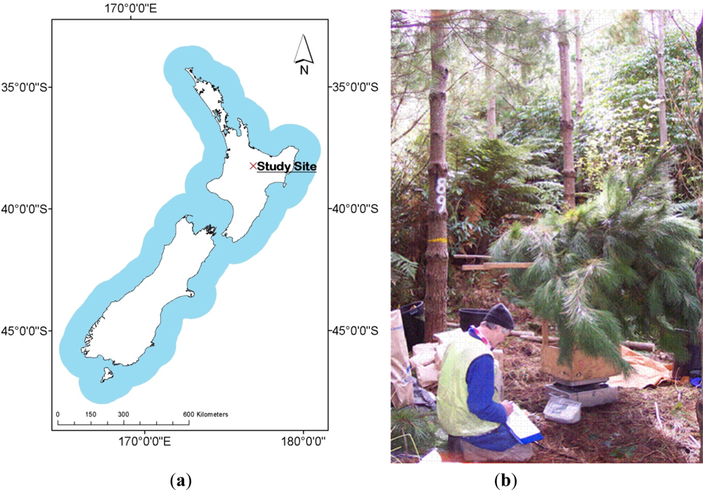
This forest was selected because Beets et al. had previously measured radiata pine biomass and assessed understorey height in field plots within the forest [6]. Foliage density (expressed as LAD) was measured in 2 m height bands across ten 0.16 ha field plots by sampling representative trees. The plots were approximately square. From these data vertical regions could be generally described as pine foliage, understorey and ground. Each plot was planted with the same stocking in 1997, and had received the same silviculture. Five representative sample trees per plot were felled from 21 August to 8 September 2006. The fact that these trees were felled prior to the LiDAR flight is unfortunate, but due to the large plot size (and number of trees) the overall effect was marginal. Tree crowns were weighed fresh in the field by 2 m height zone, measured from the base of each tree. Fifty needle fascicles were sampled randomly from each height zone and stored in polythene bags with water. Sample branches from each 2 m height zone were also weighed fresh in the field, and partially dried to aid with separation of needles from branches. Needles were oven dried to constant weight at 65 °C and weighed. Leaf area of the 50 fascicles per 2 m height zone was determined on an all-surfaces basis from fascicle length and volume, using methods described in Beets and Lane [22], and then oven-dried and weighed. LAD by 2 m height zone was calculated for each zone by multiplying the fascicle dry weight by the specific leaf area of the 50 fascicles. The leaf area index per plot was obtained using the basal area ratio method, where the sum of zonal leaf areas of sample trees per plot is multiplied by the plot basal area, divided by the sample tree basal area [23]. Figure 1(a) shows the field trial location and Figure 1(b) shows the foliage measurement.
2.2. Waveform Analysis
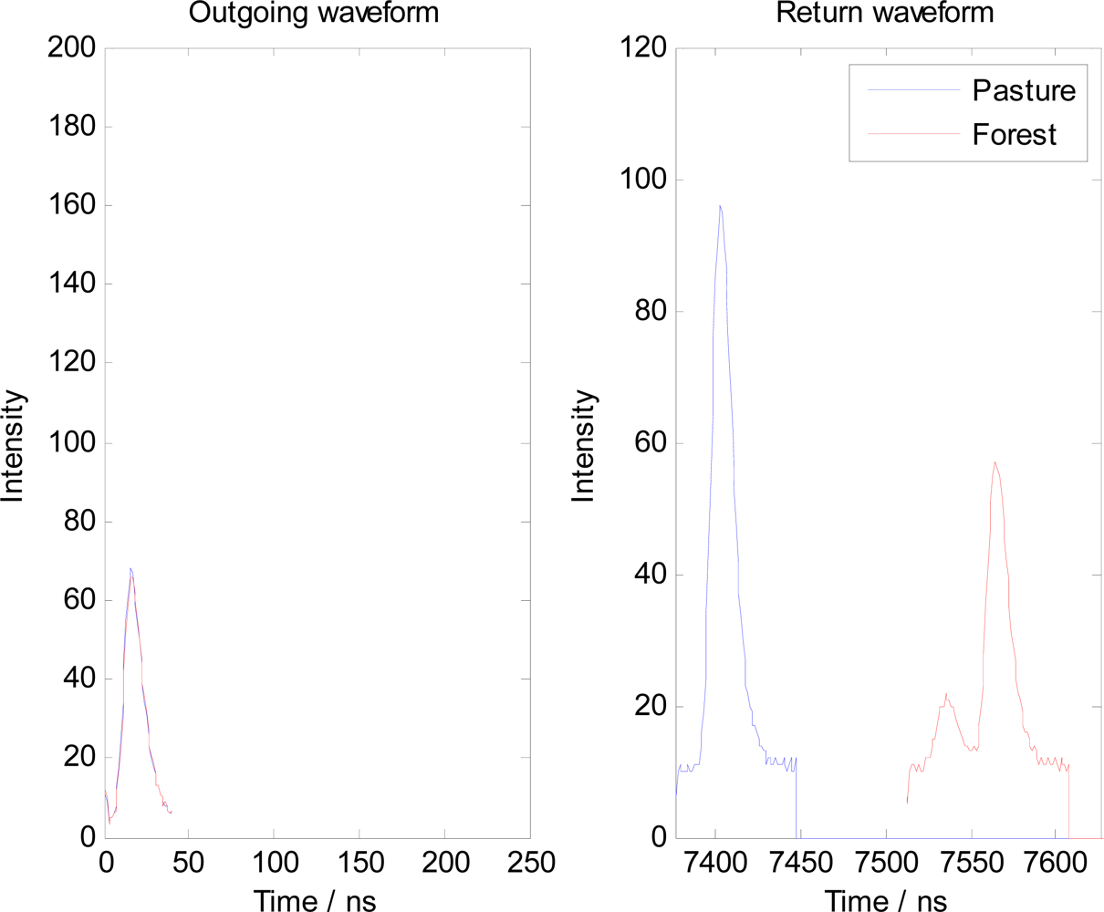
Figure 2 shows two waveform sections, exactly as read out of the raw waveform LiDAR file, one over open pasture and one over forest. The outgoing and return waveforms are shown for both.
Two things immediately distinguish the waveform over forest from the waveform over open pasture:
- The forest waveform consists of multiple peaks (returns)
- The peak intensities (in arbitrary units defined by the hardware) of the forest waveform are less than the open pasture.
These two observations are common, but do not unambiguously distinguish a return from forest cover from a return from pasture. Many forest waveform traces may yield only one peak, and in many cases the peak amplitude of the forest return may be greater than that from pasture. There is a general similarity between the peaks in both traces that is driven by the shape of the outgoing pulse. If we remove the dominance of the outgoing pulse from the return signal then more information can be learned about the target. Also of note in the figure is the almost exact similarity of the outgoing waveforms, and the similarly in width of the outgoing pulse and the return from pasture. It is odd that the return waveform in this case has a stronger intensity than the outgoing pulse (which if genuine would imply that extra energy were somehow added into the system), but this is in fact due to the way in which the outgoing pulse is sampled and the reflected and outgoing intensity units should not be considered equal.
Jutzi and Stilla [11] described the return waveform y(t) as a convolution of the surface response v(x,y,z), the outgoing pulse o(t), the response of the measurement unit m(t), the spatial beam distribution p(x,y), and a background noise n(t). If the pulse is timed and we know the plane’s position and scan angle in three dimensions (i.e., we can describe x,y and z as a function of t) then we can describe v(x,y,z) as v(t).
p(x,y) is approximately a Gaussian on a flat surface, however it is impossible to resolve horizontal detail within one single footprint. Thus we make the necessary assumption that our measurements of interest (e.g., foliage density) vary on a scale significantly greater than the footprint size. This allows the simplification that the illuminated surface is approximately homogeneous across the width of the beam footprint, and consequentially we can ignore any bias caused by greater illumination at the centre of the beam and treat p(x,y) as a constant. Furthermore, comparison of the outgoing pulse o(t) with the return waveform y(t) for large flat surfaces (a pond on a windless day) shows that m(t) is negligible compared to o(t) [21]. This leaves us with
which may be solved for the surface response v(t) by a Wiener deconvolution where we estimate g(t) to minimize the error in our estimation of v(t), so that
The Weiner deconvolution filter can be used to find g(t), shown here in the frequency domain
where S(f) is the mean power spectral density of the outgoing pulse o(t). N(f) is the power spectral density of the noise n(t). An estimate of the background noise n(t) is obtained from waveform sample values far away from any return. Equation (3) may then be solved to obtain v̂(t), referred to as the deconvolved waveform. If the target were completely flat, orthogonal to the scan angle, solid and 100% reflective, the “perfect” deconvolution would yield a delta function coincident with the start (not the peak) of the convolved waveform. This shift of the peak on the time axis could lead to incorrect range measurements unless the results were calibrated to a known reference height, although such calibrations are a standard part of any LiDAR data acquisition. However, vegetation is neither flat nor solid. Neither is it 100% reflective, so the deconvolved waveform will always have a finite width. Figure 3 shows the two example waveforms in Figure 2 in both deconvolved and original forms. In both cases, it is apparent that the deconvolved waveform is noisier than the original waveform, because noise is amplified in the deconvolution process. However, the peak is also noticeably less blurry, having removed (to the extent possible) the effects of the broad transmit pulse to obtain the estimate of the surface response. It is also apparent that our implementation of the Wiener filter introduces the aforementioned shift (i.e., the output signal is slightly advanced with respect to the input), but due to the fact that the target was not solid, flat or completely reflecting (as was the case also with the background noise), this peak has a finite width and is not shifted all the way to the start of the original peak (this ideal is closer represented in the return from pasture). This is because all the nanosecond samples of the transmit pulse would have been reflected from a range of depths, only a small proportion of which would have been from the very top of the target. The deconvolved waveform is a truer representation of the actual surface response.
Once we have obtained a deconvolved waveform (using the outgoing waveform), this may be analyzed so that characteristic metrics may be recorded. The metrics employed in this study to describe each return are: height above ground, peak height, peak width (evaluated as a Gaussian half-height width) and the exponential decay constant of the return shape between the peak and the next local minima. This study aims to show that peak height and width will be affected by shadowing deep in the canopy (and not be a good discriminator), but that exponential decay rate will be less affected (see results and discussion). The method of obtaining these is:
- Georeference every 1 ns waveform sample to determine which waveforms (or part waveforms) fall into the field plots.
- Determine a ground surface for the field plots.
- Employ Gaussian fitting to describe each peak with a peak height and half-height width.
- Employ exponential curve-fitting to determine the exponential decay rate of each peak.
- Determine the above ground height of each peak (for comparison with field measured foliage data).
- was achieved using the methods and code in Parrish [21], adapted for the New Zealand NZGD2000 coordinate system. The field plots were located using a high-grade, differentially-corrected GPS unit, and the selection of waveform samples simply consisted of any that fell into the vertical space above the field plots.
- was achieved by using the discrete LiDAR data set for the area flown. The ground-filtering algorithm (GroundFilter.exe) in FUSION [24] was used to select only ground returns (based on the linear filtering method of Kraus and Pfeifer [25]). These ground returns were interpolated into a raster using FUSION’s GridSurfaceCreate.exe algorithm.
- As we are interested in decay rates of waveform peaks in (4), we do not need to search for additional ‘hidden’ peaks as other authors have. Peaks that are hidden through close proximity to another or low peak amplitude will not have sufficient data points after the peak to give a good decay. As such, we only select peaks in the waveform data with a corresponding discrete return. Gaussians were fit using Matlab’s fminsearch function, a simplex search method given in [26]. This is a direct search method that does not use numerical or analytic gradients. The number of Gaussians and a first-guess of their locations could be specified by the number and location of returns in the discrete datset. The peak height and half-height width of each Gaussian is recorded, as well as the R2 value of the fit.
- In (3), the location of each peak to be analyzed will have been determined. An exponential curve fit of the type y = Ce−λx was applied from the peak maximum to the following local minima (either before the end of the waveform or before the next peak). The exponential curve was determined, also using Matlab’s fminsearch algorithm, taking the peak maximum as a start point for C, and 0.2 as a start point for λ. The final value for λ is recorded along with the R2 value of the fit.
- As this study is a proof of concept, only peaks that corresponded to a return in the discrete data set were analyzed (see step 3). Ground height was obtained by linear interpolation of the ground surface generated in (2) to the discrete return’s x, y coordinates. Height above ground was the discrete return height, minus the interpolated ground height. We made the assumption that the waveform peak was coincident with the discrete return, which is appropriate, as the ALTM discrete return data and waveform data were generated from the same input signal. Using the coordinates from the well-calibrated discrete return data eliminated small potential errors from georeferencing the waveform, as the ranging calculation was calibrated on the convolved peak, and not the translated peak observed in the deconvolution. Waveform LiDAR is known to give many more returns than discrete LiDAR, so by only selecting returns with a corresponding discrete return we are limiting our results to only the strongest peaks available. This should demonstrate any correlations most clearly, which may be hidden when including additional peaks with limited data due to close proximity to another peak or very low amplitudes.
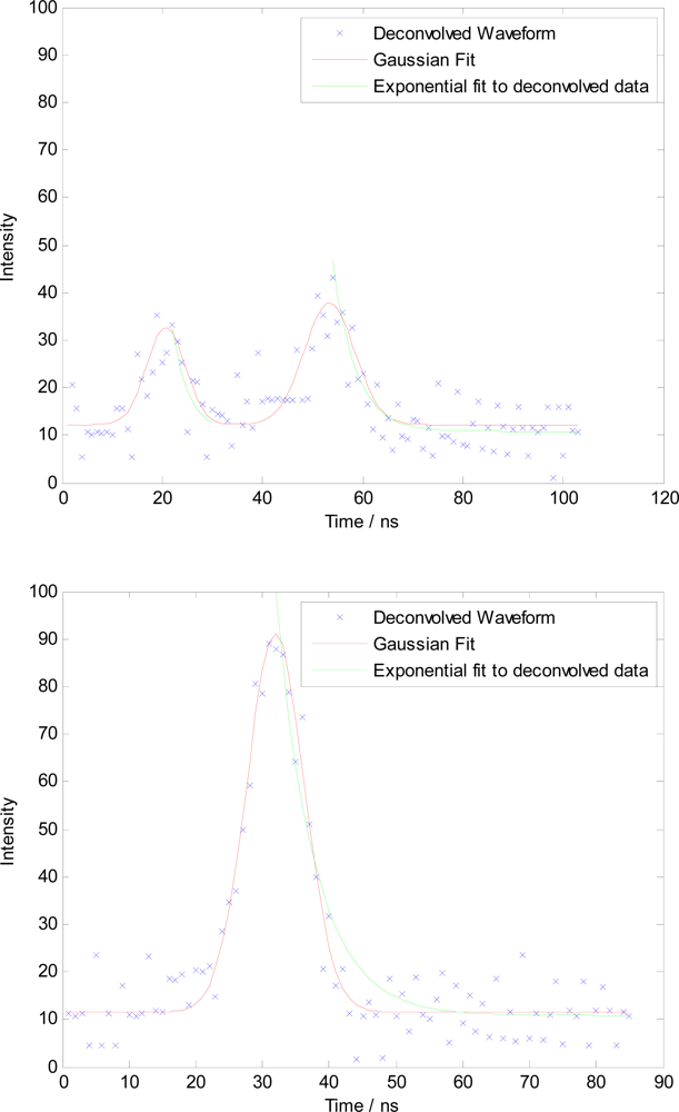
The net result of this analysis is an attribute table for each discrete return. Unlike standard discrete returns, which are described only by their coordinates and an intensity (excluding secondary processing such as classification), each return will also be assigned a Gaussian peak height, mid-height width, decay rate and height above ground. Additionally, the R2 value of both the Gaussian fit and the exponential curve fit is calculated relative to their recorded values. Our variable of interest—the vegetation type causing each reflection—is not known for each return, but is known to be a function of height. In each plot the ground existed at 0 m by default (±1 m to account for the 1 m × 1 m resolution of the DTM and inaccuracies in the filtering process), broadleaved understorey and ferns existed in the first 4 m above ground (as measured in the field), and radiata pine foliage existed above 4 m (except in one plot where a small amount was found down to 2 m). Figure 4 gives two examples of waveforms that have had the Gaussian and exponential curve fits performed. Note that the red line is the Gaussian curve fit, not the original convolved waveform, hence the reason why there is no shift in the peak.
2.3. Metric Analysis
As this study is a proof of concept, only the best peaks were selected, as poor peaks (with a low signal-to-noise ratio) are prone to poor curve fits and hence will mask any potential correlations. As a result of the amplification of background noise created through deconvolution, only waveforms with at least one intensity measurement greater than 25 (SNR > 2) were selected for analysis. After analysis, any peaks for which either the Gaussian fitting or the exponential curve-fitting yielded an R2 value of less than 0.75 were excluded from the final results. If a distinguishing metric can be found for these peaks, then it can subsequently be tried on increasingly ambiguous peaks that are harder to extract from the background noise, to find the point at which the correlation is no longer tenable. Once all metrics were collected for all suitable peaks, they were each plotted against height in bivariate frequency distributions. These are effectively two-dimensional histograms, and show how the distribution of results for each metric varies with height. After checking for any height trends (which may be used to distinguish individual returns as foliage, understory or ground), the peaks in each 2 m height band were compared—as an average—against field sampled LAD.
3. Results and Discussion
136,191 waveforms were incident over the ten 0.16 ha plots analyzed. 127,167 of these had an intensity greater than 25 (93%), in which 173,129 returns were identified and analyzed, giving approximately 1.4 returns per waveform. A further 121,051 of these were discarded, as the R2 values of either (or both) the Gaussian and exponential curve fits were less than 0.75 (Table 1). As this study is a proof of concept, only the cleanest, clearest peaks were used. If a metric of interest can be found to clearly relate peaks to their targets, then it can then be trialed on peaks with greater ambiguity.
3.1. Gaussian Peak Height
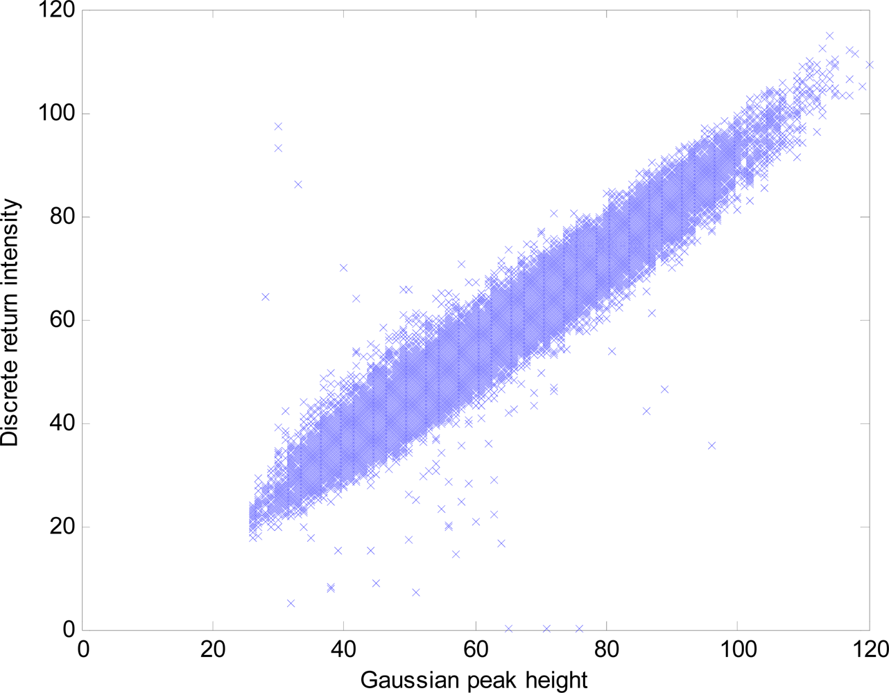
Figure 5 shows the Gaussian peak height vs. discrete return intensity for all plots. Although there is a small amount of variation, it is apparent that the discrete return intensity recorded by this unit is based on peak amplitude. The small amount of variation is due to Gaussian fitting being based on the deconvolved waveform, whereas the discrete return intensity is based on convolved data.
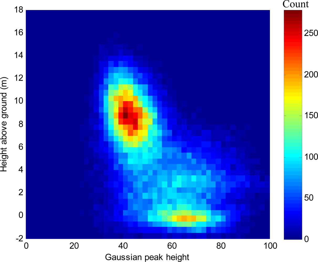
Figure 6 shows how values for Gaussian peak height vary with height above ground as a bivariate frequency distribution, where color indicates frequency at that combination of height and intensity. Two major groupings are apparent—medium intensity returns 6–12 m above the ground, and higher intensity returns at ground height. Note that some returns may have a negative height above ground due to the coarser resolution of the DTM (1 m) and inaccuracies in the filtering process. Even so, these groupings show that ground returns generally have a higher intensity than coniferous canopy returns, which is a well-known result. Furthermore, there is a smaller number of higher intensity returns occurring around 2–4 m above the ground that are likely to be the broadleaved understorey present in the stand in that height band. Due to the larger, flatter surface, broadleaved plants are also known to give stronger returns than pine needles. Although Figure 6 shows that there is a trend for returns from the ground to have peak heights greater than returns from foliage, the distributions for each surface type overlap considerably. This means that whilst the average from a collection of pulses can be used to infer whether a volume is ‘ground’ or ‘foliage’, it cannot be used to assign more than a probability to each individual return. Furthermore, where volumes contain a mixture—such as foliage and stems, or canopy and understorey—peak height will not be able to separate returns from each. The variation in peak intensity for returns from the same surface type is explained by the complexity and multitude of incident angles and paths that the pulse may take. For example, a return from a pulse with a high angle of incidence to the reflecting surface would be expected to have a lower intensity and wider peak than a return from a pulse that struck the same surface orthogonally. If all surfaces were horizontal then the angle of incidence would be the scan angle—for which no correlations were found against any of the derived metrics—however as few surfaces were truly horizontal, we cannot discount the effect of incidence angle. Similarly, a return from close to the ground is likely to come from a beam that has already been attenuated and perhaps already yielded a return or more. In this experiment, trying to account for previous returns did not improve the discriminating power of intensity, probably due to many smaller attenuation events that didn’t result in a return, and the fact that it appears that a strong reflector (such as the ground) can still yield a strong return even when the beam is heavily attenuated. The nature of the relationship between intensity, target characteristics and attenuation is too complex for a thorough investigation here, and could be better determined in controlled laboratory conditions (see Section 4).
3.2. Gaussian Half-Height Width
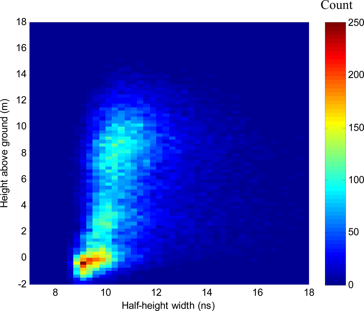
Figure 7 shows the bivariate frequency distribution for Gaussian half-height width vs. height above ground over all plots. There is an apparent trend for peaks from the canopy to be slightly wider, although returns in the 0–4 m band which is dominated by understorey show a wide range of widths. As in the case of peak height however, the distribution for canopy overlaps the distribution for ground. This means that individual pulses cannot be differentiated by width, but average values may be used over larger volumes.
3.3. Pulse Decay Rate
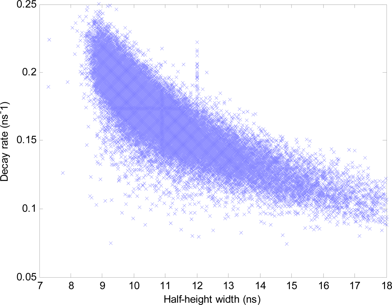
Figure 8 shows the bivariate frequency distribution for pulse decay rate vs. height above ground over all plots. There is a trend for decay rate to be highest (i.e., faster decay, lower transmissivity) on the ground, and less so for the understorey and even less for the foliage, implying that foliage is more likely to transmit light than the ground. These results correspond with the earlier finding that peaks relating to returns from the canopy were generally wider than those from the ground. Figure 9 shows a plot of half-height width vs. decay rate, confirming that the two are correlated variables. Neither peak height, nor half-height width, nor decay rate have shown conclusive separation between returns from foliage, ground or understorey. As it is impossible to know in this data which returns were from stems and which were from foliage, it is unknown whether any of these metrics can individually distinguish between them. Given that none of these metrics can conclusively distinguish individual returns from the ground from those from foliage, the chances are slim.
3.4. Comparison with Foliage Density
We cannot compare individual pulse metrics with LAD values as LAD was defined over a larger volume, but we can compare average LAD over a volume with average parameter values. Figure 10 shows how LAD varied by height for the ten plots. Understorey was not included in the LAD measurements, although its height was noted and did not exceed 4 m.
We will not investigate the LiDAR metric values below 4 m that will be affected by understorey. Also, we will exclude bands where the LAD <1 m2 per m3 because the foliage is so sparse that most LiDAR pulses will simply miss it. Figure 11(a–d) shows the average values for these LiDAR metrics in each height band vs. the LAD for the respective height bands, along with a line of best fit and an R2 value for the fit.
Figure 11 shows that none of the LiDAR metrics discussed here—discrete return intensity value (automatically derived in the hardware from the convolved waveform maxima), deconvolved peak height (based on Gaussian curve-fitting), half-height peak width (again from Gaussian fitting) and decay rate (from fitting an exponential to the downslope of the peak)—have an exceptionally strong correlation with average LAD over the height band. This is somewhat expected, as here LAD is defined over a volume of 3,200 m3, but varies substantially in localized regions (i.e., close to a branch vs. far from a branch). As the reflection from a LiDAR footprint (and any metrics derived from it) is defined over a volume of around ∼0.03 m3, it will be determined by the local value not the wider-scale average. Hence, individual values will vary, but if the sampling were fair, the average values of any metrics indicative of LAD should show strong correlations with the average value of LAD. However, sampling was not fair, as a return will only be registered if the pulse encounters sufficient material in one sample volume, thereby creating a tendency to overestimate LAD in more vegetated volumes. However, the fact that there is a moderate correlation between average decay rate and LAD is scientifically interesting. Note that as mentioned in Section 2.3, this correlation is only for the peaks with high intensities and good curve fits (R2 values > 0.75). It is interesting to see what happens to this correlation when we allow more peaks into the analysis. If we drop the R2 requirement for curve-fitting to >0.65, the correlation between the average decay rate and LAD drops to an R2 of 0.17, whilst the number of peaks analyzed rises from 52,078 to 80,957. If we drop the requirement that the waveforms analyzed have an intensity >25 and instead take all waveforms with an intensity >15 and curve-fitting R2 > 0.65, the R2 for average decay rate to LAD drops to 0.16. This demonstrates how sensitive the metrics are to curve-fitting quality, and justifies the subset of peaks analyzed in this study. So, although the relationships are weak and only visible with an optimum carefully selected subset of the data, the fact that a relationship between LAD and decay rate can be observed even with heavy caveats is interesting and points towards a new way of thinking about LiDAR returns.
3.5. Models for Interpreting Waveform Shape
There are two ways that waveform LiDAR of a vegetated area may be interpreted:
- The standard interpretation is as the result of a series of discrete ‘hard’ returns, such as may be achieved by well-separated layers of foliage. These supposed layers are of a thickness equal to or less than the return distance travelled by the laser pulse in one sampling period (0.15 m for 1 ns sampling).
- As the result of transmission and reflectance from a volume of semi-transparent foliage which attenuates the radiation exponentially.
Clearly, the discrete Gaussian interpretation becomes similar to the volumetric interpretation once the separation of the Gaussians is equal to or less than the sampling period. Previous authors have used Gaussian fitting to distinguish a small number of returns separated by significantly more than the sampling period [15–18]. These returns are normally characterised by their peak height and also occasionally by their width (whether standard deviation, half-height width etc.), which have been used to differentiate returns between trees in mixed species stands [16]. The radiata pine in this study—or any tree to the authors’ knowledge—can neither be accurately described as a series of thin, well-separated layers of 0.15 m of less in thickness, nor as a homogeneous, diffuse cloud of material. Given that the beam footprint in most aerial LiDAR applications is typically ∼0.2 m, a 1 ns sampling period will lead to each sample being the integrated response of a roughly cylindrical region of space ∼0.15 m tall and ∼0.2 m in diameter. Thus, a lack of homogeneity at scales smaller than this (such as the scale of needles) is not relevant. If the tree could be thought of as a “gas” of needles and small elements ≪0.2 m then a semi-transparent gas model could be used as a first-order approximation. In this model the transmissivity (T) of the semi-transparent medium can be described by the Beer-Lambert Law
where IT is the transmitted intensity, I0 is the initial intensity, α is the absorption coefficient and x is the distance travelled through the gas. At a depth x into the canopy, a constant proportion (R) of the incident light will be reflected. We assume Lambertian reflectance, and that this is further attenuated by the gas as it leaves. IR at the surface is then given by
Thus, we see that if each canopy sample is of a constant density and distribution, it will have an absorption coefficient α, and as foliage density increases, so does α. This means that we can explain why an exponential decay in intensity for each return will be correlated with the foliage density. Although this is only a first-order approximation, it gives a conceptual model to explain the observations of this experiment and also those of Wagner [18] and Chauve [14], who note a skew to some returns over vegetation. Whether a robust relationship can be determined between LAD and decay constant which is applicable over a range of forests is beyond the scope of this study, and should be investigated in future studies.
The benefit of using an exponential decay rate is that it is not affected by shadowing. Shadowing affects both peak height and peak width due to the reduction in irradiance incident on lower surfaces. This—along with the complex nature of the surfaces—contributes to the observed variation in values for the same surface with these metrics. Ideally, shadowing could be accounted for by the summation of all samples in a waveform prior to the peak. However, much of the actual attenuation will not lead to a reflected signal at the sensor distinguishable from the background noise. This problem could be solved by equipment that is more sensitive and perhaps a different frequency laser, but such changes come with other issues and are not currently in the public domain. In the absence of an intensity-based method to account for shadowing, decay rate gives valuable information that is not affected by it. In summary, this interpretation provides insight into our observation that waveform decay rate has the potential to determine foliage density when averaged over a local area, bypassing some of the issues of using variables based on pulse intensity. Furthermore, if LAD can be shown to be moderately correlated with other (independent) metrics selected for that species and site (such as Normalized Difference Vegetation Index from aerial imagery), then the inclusion of spatially-averaged decay rate in a multiple regression may enable very robust estimates.
4. Conclusions
The primary aim of this study was to investigate whether waveform shape could be used to identify the source of individual LiDAR returns from forested landscapes. Waveform shape was quantified by means of various curve-fitting methods such as a peak height, half-height width and exponential decay rate, which were attributed to each return, significant enough to trigger the discrete-return sensing system. A subset of these with the best signal-to-noise ratio (SNR > 2) and curve fits (R2 > 0.75) were used to remove additional variability in the metrics, justified, as this study is a proof of concept at this stage. Due to the complexity of the surfaces and multitude of angles, textures and paths etc., each waveform shape metric showed more potential variation within a surface type than it did between surface types. This negates the possibility of identifying the source of individual returns.
Three-dimensional spatial averages of these waveform metrics were shown to give indications of surface type over larger areas and volumes. For example, ground returns on average presented waveforms with higher peaks, shorter widths and faster decays. Foliage returns conversely averaged lower peaks, wider pulses and slower decays. Decay rate showed the best correlation with average Leaf Area Density (defined in 2 m height bands over a 0.16 ha plot), when the average value for all returns in each volume was obtained. A linear correlation with an R2 value of 0.37 was obtained. Although moderate, this correlation indicates that the spatially-averaged decay rate may be beneficial in estimating LAD, especially if it can be combined with other (independent) metrics in a multiple regression analysis. When less stringent criteria for selecting peaks were used, the strength of this correlation dropped.
To explain the correlation between the exponential decay of returns and the LAD, a model was presented which approximates the canopy as a semi-transparent gas, and utilizes the Beer-Lambert Law to model the exponential decay of reflected intensity. This model has merit when used in conjunction with the standard interpretation of waveform LiDAR over vegetation, which explains the returns as a series of discrete layers leading to a one-dimensional Gaussian mixture. To further evaluate this model and to develop a robust correlation between foliage density and waveform decay rate, further testing is required. It may be advantageous to conduct this testing in a controlled environment, such as a laboratory, where small foliage samples may have LAD and occlusion measured precisely and then be scanned by LiDAR. This laboratory testing should also enable us to better quantify the extent of spatial averaging needed to an obtain optimal balance between the competing goals of accuracy and localization in our LAD estimates.
Acknowledgments
The work in this paper was funded by the Scion Capability Fund and used data collected by the Ministry for the Environment. Many thanks to Nigel Searles from the Ministry for the Environment for use of the data, and to Andrew Dunningham, Jonathan Harrington and David Pont from Scion for their help and knowledge. Particular thanks must also go to New Zealand Aerial Mapping, in particular Tim Farrier, for providing an excellent LiDAR service and for assistance with countless queries and demands.
References
- Sithole, G.; Vosselman, G. Experimental comparison of filter algorithms for bare-earth extraction from airborne laser scanning point clouds. ISPRS J. Photogramm 2004, 59, 85–101. [Google Scholar]
- Meng, X.; Currit, N.; Zhao, K. Ground filtering algorithms for airborne lidar data: A review of critical issues. Remote Sens 2010, 2, 833–860. [Google Scholar]
- Lefsky, M.A.; Harding, D.J.; Keller, M.; Cohen, W.B.; Carabajal, C.C.; Espirito-Santo, F.D.B.; Hunter, M.O.; de Oliveira, R., Jr. Estimates of forest canopy height and aboveground biomass using ICESat. Geophys. Res. Lett 2005, 32, L22S02. [Google Scholar]
- Naesset, E. Estimating timber volume of forest stands using airborne laser scanner data. Remote Sens. Environ 1997, 61, 246–253. [Google Scholar]
- Maclean, G.; Krabill, W. Gross-merchantable timber volume estimation using an airborne lidar system. Can. J. Remote Sens 1986, 12, 7–18. [Google Scholar]
- Beets, P.N.; Reutebuch, S.; Kimberley, M.O.; Oliver, G.R.; Pearce, S.H.; McGaughey, R.J. Leaf area index, biomass carbon and growth rate of radiata pine genetic types and relationships with lidar. Forests 2011, 2, 637–659. [Google Scholar]
- Stephens, P.R.; Watt, P. J.; Loubser, D.; Haywood, A.; Kimberley, M.O. Estimation of Carbon Stocks in New Zealand Planted Forests Using Airborne Scanning Lidar. ISPRS Workshop on Laser Scanning 2007 and SilviLaser 2007, Espoo, Finland, 12–14 September 2007; pp. 389–394.
- Reitberger, J.; Schnörr, C.; Krzystek, P.; Stilla, U. 3D segmentation of single trees exploiting full waveform lidar data. ISPRS J. Photogramm 2009, 64, 561–574. [Google Scholar]
- Morsdorf, F.; Kotz, B.; Meier, E.; Itten, K.; Allgower, B. Estimation of LAI and fractional cover from small footprint airborne laser scanning data based on gap fraction. Remote Sens. Environ 2006, 104, 50–61. [Google Scholar]
- Chasmer, L.; Hopkinson, C.; Treitz, P. Investigating laser pulse penetration through a conifer canopy by integrating airborne and terrestrial lidar. Can. J. Remote Sens 2006, 32, 116–125. [Google Scholar]
- Jutzi, B.; Stilla, U. Characteristics of the measurement unit of a full-waveform laser system. Revue Française de Photogrammétrie et de Télédétection 2006, 182, 17–22. [Google Scholar]
- Reitberger, J.; Krzystek, P.; Stilla, U. Analysis of full waveform lidar data for the classification of deciduous and coniferous trees. Int. J. Remote Sens 2008, 29, 1407–1431. [Google Scholar]
- Parrish, C.E.; Jeong, I.; Nowak, R.D.; Smith, R. Empirical comparison of full-waveform lidar algorithms: Range extraction and discrimination performance. Photogramm. Eng. Remote Sensing 2011, in press. [Google Scholar]
- Chauve, A.; Vega, C.; Durrieu, S.; Bretar, F.; Allouis, T.; Deseilligny, P.; Puech, W. Processing full-waveform lidar data in an alpine coniferous forest: Assessing terrain and tree height quality. Int. J. Remote Sens 2009, 30, 27. [Google Scholar]
- Hofton, M.A.; Minster, J.B.; Blair, J.B. Decomposition of laser altimeter waveforms. IEEE Trans. Geosci. Remote Sens 2000, 38, 1989–1996. [Google Scholar]
- Reitberger, J.; Krzystek, P.; Stilla, U. Analysis of Full Waveform Lidar Data for Tree Species Classification. In International Archives of Photogrammetry, Remote Sensing and Spatial Information Sciences, Symposium of ISPRS Commission III “Photogrammetric Computer Vision PCV '06”, Bonn, Germany, 20–22 September 2006; 2006; 36, pp. 228–233. [Google Scholar]
- Persson, Å.; Söderman, U.; Töpel, J.; Ahlberg, S. Visualization and Analysis of Full-Waveform Airborne Laser Scanner Data. In International Archives of Photogrammetry, Remote Sensing and Spatial Information Sciences, ISPRS WG III/3, III/4, V/3 Workshop “Laser scanning 2005”, Enschede, The Netherlands, 12–14 September 2005; 2005; 36, pp. 103–108. [Google Scholar]
- Wagner, W.; Ullrich, A.; Ducic, V.; Melzer, T.; Studnicka, N. Gaussian decomposition and calibration of a novel small-footprint full-waveform digitizing airborne laser scanner. ISPRS J. Photogramm 2006, 60, 100–112. [Google Scholar]
- Jupp, D.; Culvenor, D.S.; Lovell, J.L.; Newnham, G.J.; Strahler, A.H.; Woodcock, C.E. Estimating forest LAI profiles and structural parameters using a ground-based laser called ‘Echidna®. Tree Physiol 2009, 29, 171–181. [Google Scholar]
- Drake, J.B.; Dubayah, R.; Clark, D.B.; Knox, R.G.; Blair, J.B.; Hofton, M.A.; Chazdon, R.L.; Weishampel, J.F.; Prince, S. Estimation of tropical forest structural characteristics using large-footprint lidar. Remote Sens. Environ 2002, 79, 305–319. [Google Scholar]
- Parrish, C.E. Vertical Object Extraction from Full-Waveform Lidar Data Using a 3D Wavelet-Based Approach. Ph.D. Thesis, The University of Wisconsin-Madison, Madison, WI, USA; 2007. [Google Scholar]
- Beets, P.; Lane, P. Specific leaf area of pinus radiata as influenced by stand age, leaf age, and thinning. New Zealand J. Forest. Sci 1987, 17, 283–291. [Google Scholar]
- Madgwick, H. Above-ground dry-matter content of a young close-spaced pinus radiata stand. New Zealand J. Forest. Sci 1981, 11, 203–209. [Google Scholar]
- McGaughey, R.J. Fusion. US Pacific Northwest Research Station, Forest Service: Salt Lake City, UT, USA, 2010. Available online: http://www.fs.fed.us/eng/rsac/fusion/ (accessed on 7 December 2011).
- Kraus, K.; Pfeifer, N. Determination of terrain models in wooded areas with airborne laser scanner data. ISPRS J. Photogramm 1998, 53, 193–203. [Google Scholar]
- Lagarias, J.C.; Reeds, J.A.; Wright, M.H.; Wright, P.E. Convergence properties of the nelder-mead simplex method in low dimensions. SIAM J. Optimiz 1999, 9, 112–147. [Google Scholar]
Figure 1.
(a) Study location in North Island, New Zealand, and (b) foliage measurement.

Figure 2.
Raw waveform data recorded from two pulses over open pasture and forest cover.

Figure 3.
Convolved and deconvolved forms of the waveforms in Figure 2 from pasture and from forest.
Figure 3.
Convolved and deconvolved forms of the waveforms in Figure 2 from pasture and from forest.
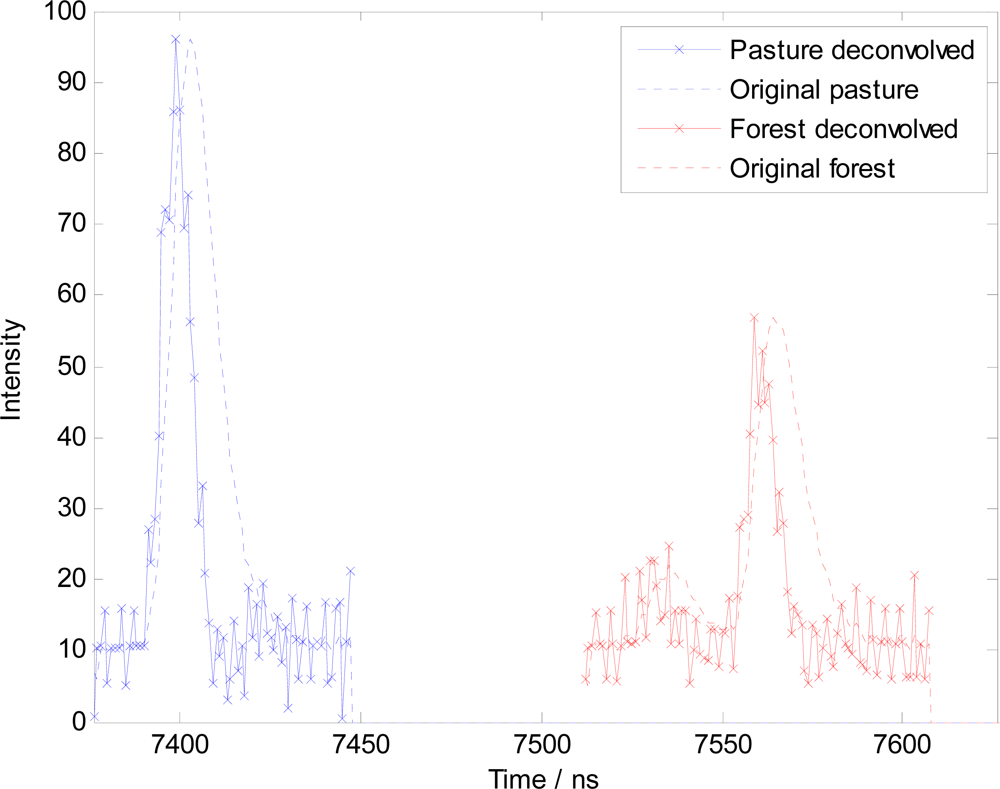
Figure 4.
Deconvolved LiDAR data (blue) with multiple Gaussian fitting (red, 1 on the left, two on the right), and decay rates of each peak estimated (green).
Figure 4.
Deconvolved LiDAR data (blue) with multiple Gaussian fitting (red, 1 on the left, two on the right), and decay rates of each peak estimated (green).

Figure 5.
Peak height of Gaussian curves fitted to deconvolved waveform LiDAR vs. corresponding discrete return intensities recorded by the discrete-return LiDAR unit.
Figure 5.
Peak height of Gaussian curves fitted to deconvolved waveform LiDAR vs. corresponding discrete return intensities recorded by the discrete-return LiDAR unit.

Figure 6.
Bivariate frequency distribution of peak height of Gaussian curves fitted to deconvolved waveform LiDAR vs. height above ground.
Figure 6.
Bivariate frequency distribution of peak height of Gaussian curves fitted to deconvolved waveform LiDAR vs. height above ground.

Figure 7.
Bivariate frequency distribution of half-height width of Gaussian curves fitted to deconvolved waveform LiDAR vs. height above ground.
Figure 7.
Bivariate frequency distribution of half-height width of Gaussian curves fitted to deconvolved waveform LiDAR vs. height above ground.

Figure 8.
Bivariate frequency distribution of decay rate of exponential curves fitted to deconvolved waveform LiDAR vs. height above ground.
Figure 8.
Bivariate frequency distribution of decay rate of exponential curves fitted to deconvolved waveform LiDAR vs. height above ground.
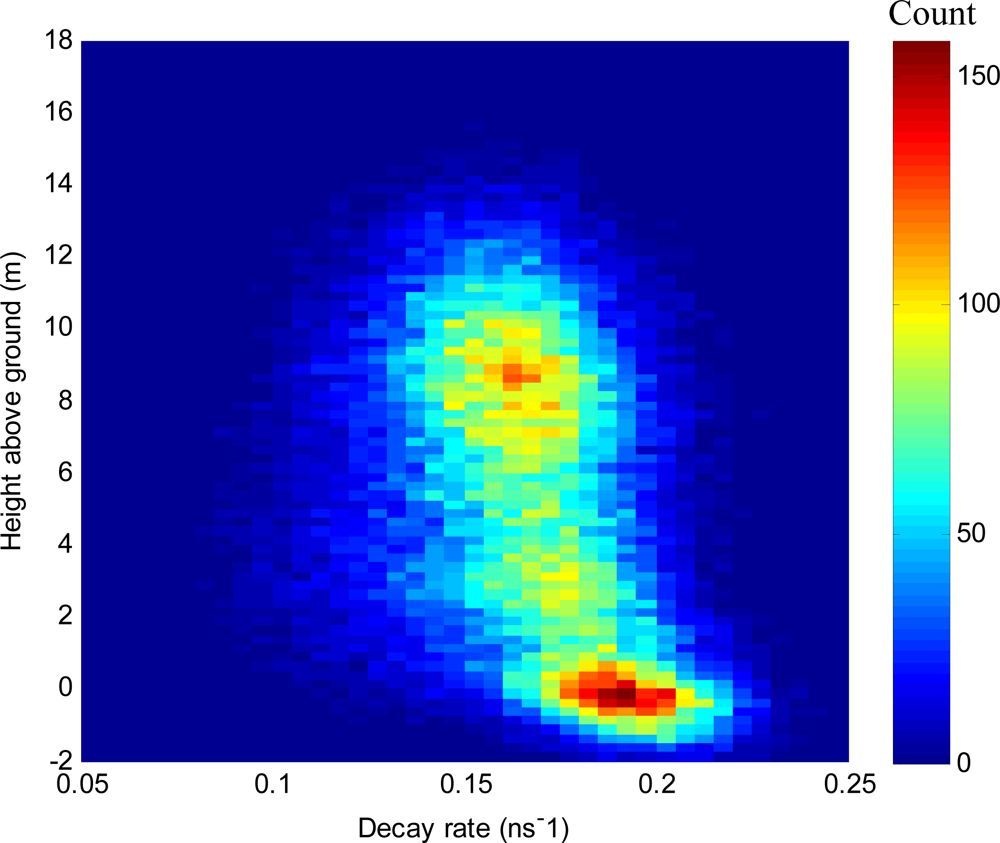
Figure 9.
Scatter plot of half-height width vs. decay rate for curve fits on deconvolved waveform LiDAR.
Figure 9.
Scatter plot of half-height width vs. decay rate for curve fits on deconvolved waveform LiDAR.

Figure 10.
Variation of Leaf Area Density (LAD) vs. height for 10 sample plots in 2 m height bands

Figure 11.
Comparison of the average value in a set of 1,600 m2 × 2 m sample plots for (a) intensity of discrete LiDAR returns, (b) peak height of deconvolved waveform LiDAR returns, (c) half-height width of deconvolved waveform LiDAR and (d) exponential decay rate of deconvolved waveform LiDAR returns, relative to the average field-measured leaf area density over the corresponding height band above ground.


| Plot | Number of Waveforms with Peak Intensity > 25 | Number of Returns | Number of Returns with Good Quality Fits and Intensity > 25 | Percentage Used |
|---|---|---|---|---|
| 1 | 12,558 | 11,616 | 4,570 | 28% |
| 2 | 16,150 | 14,939 | 5,608 | 27% |
| 3 | 12,305 | 11,261 | 4,942 | 33% |
| 4 | 11,332 | 10,286 | 4,207 | 29% |
| 5 | 12,326 | 11,075 | 4,541 | 31% |
| 6 | 13,810 | 13,130 | 5,488 | 32% |
| 7 | 12,687 | 11,992 | 4,598 | 27% |
| 8 | 14,849 | 14,210 | 4,847 | 25% |
| 9 | 15,862 | 15,145 | 8,746 | 45% |
| 10 | 14,312 | 13,513 | 4,531 | 24% |
| Total | 136,191 | 127,167 | 52,078 | 30% |
Share and Cite
MDPI and ACS Style
Adams, T.; Beets, P.; Parrish, C. Extracting More Data from LiDAR in Forested Areas by Analyzing Waveform Shape. Remote Sens. 2012, 4, 682-702. https://doi.org/10.3390/rs4030682
AMA Style
Adams T, Beets P, Parrish C. Extracting More Data from LiDAR in Forested Areas by Analyzing Waveform Shape. Remote Sensing. 2012; 4(3):682-702. https://doi.org/10.3390/rs4030682
Chicago/Turabian StyleAdams, Thomas, Peter Beets, and Christopher Parrish. 2012. "Extracting More Data from LiDAR in Forested Areas by Analyzing Waveform Shape" Remote Sensing 4, no. 3: 682-702. https://doi.org/10.3390/rs4030682