Remote Sensing of Vegetation Structure Using Computer Vision


Abstract
:
1. Introduction
2. Methods
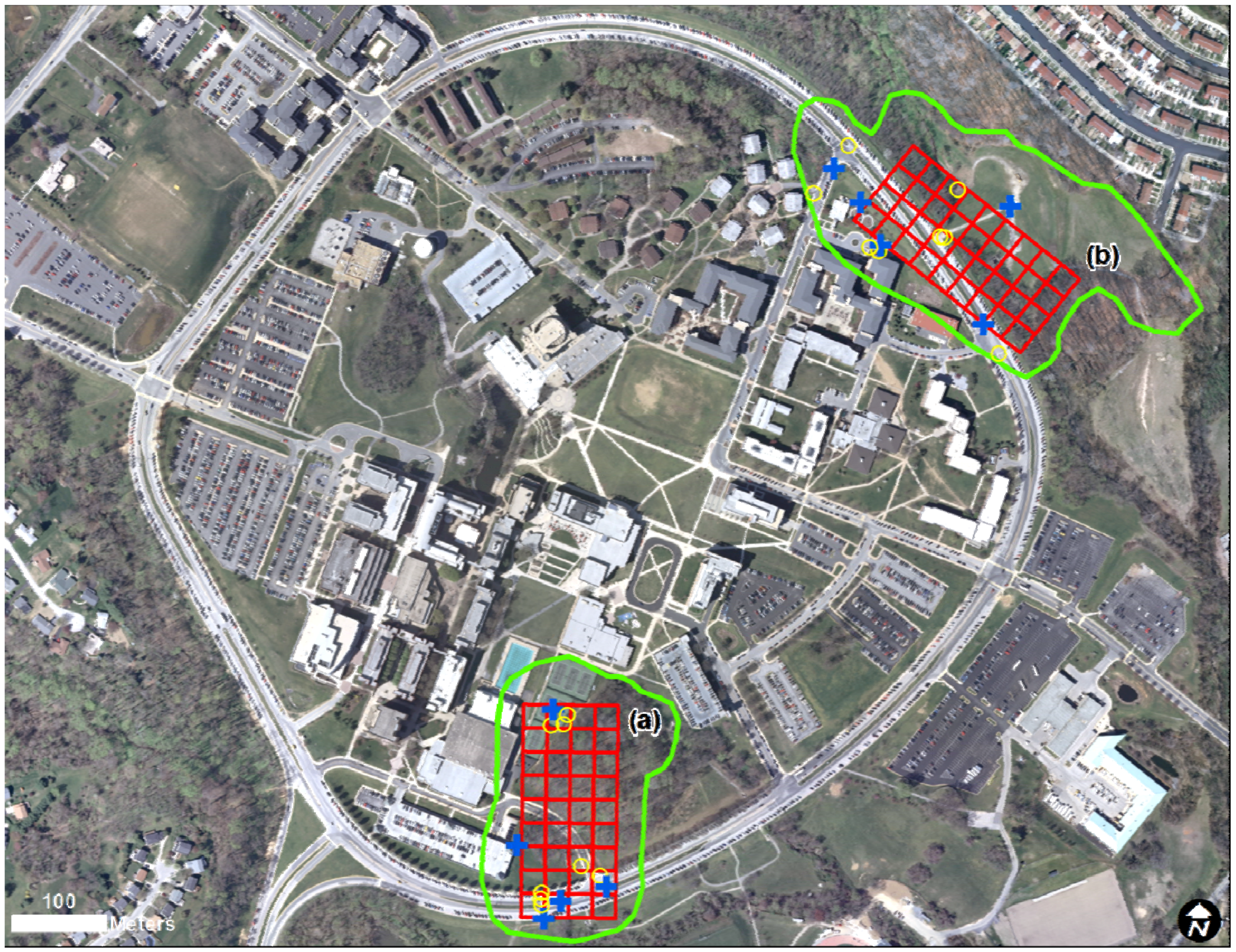
2.1. Test Sites and Field Measurements
2.2. Image Acquisition and LiDAR
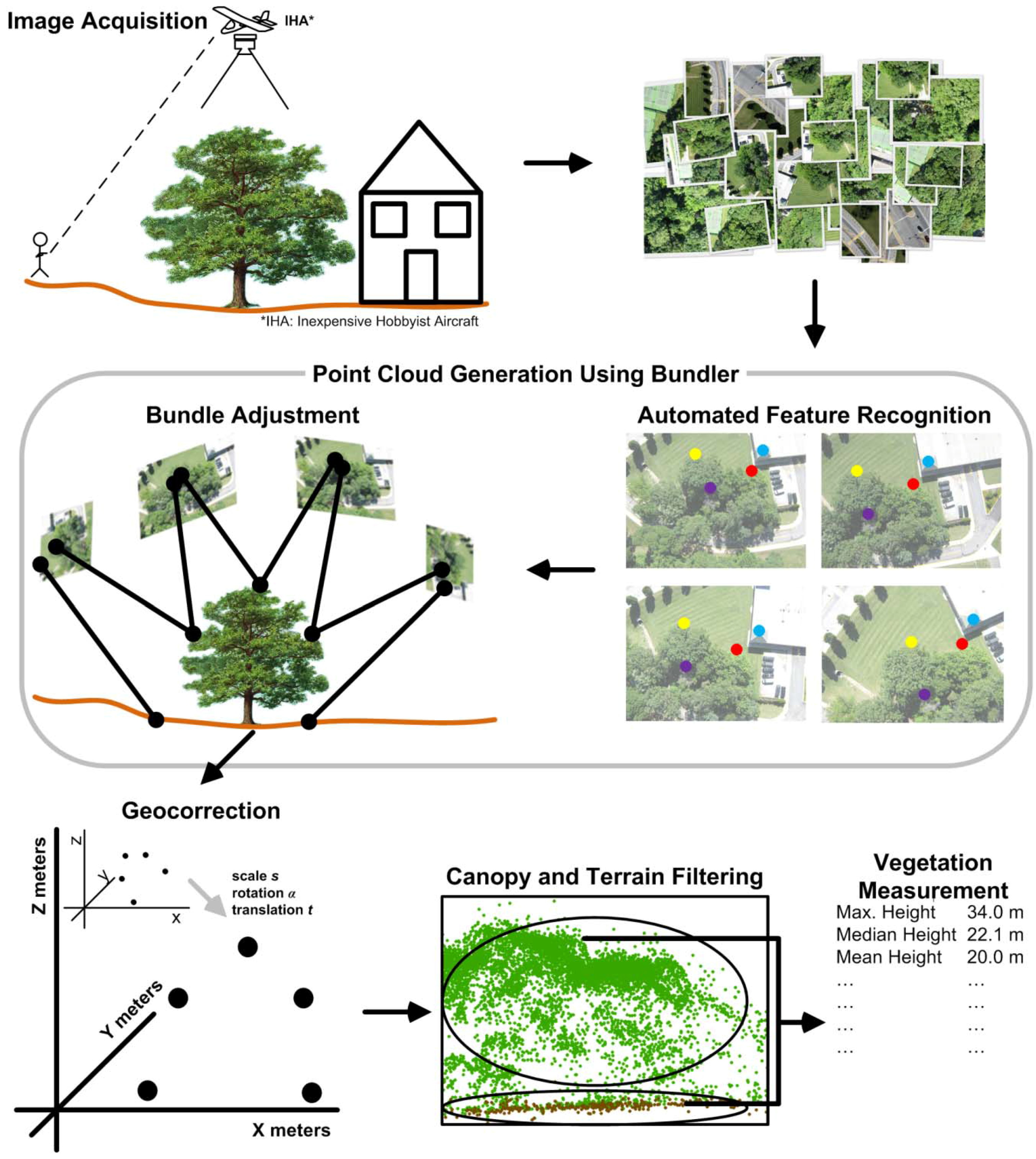
2.3. Point Cloud Generation Using Bundler

| Test site | Input images | Processing time (h) | Images selected | Keypoints | Trimmed | Outliers | Ecosynth Points | LiDAR points | ||
|---|---|---|---|---|---|---|---|---|---|---|
| Total | Ground | First return | Bare earth | |||||||
| Knoll | 237 | 2.1 | 145 | 36,524 | 2,658 | 517 | 33,349 | 1,897 | 19,074 | 15,657 |
| Herbert Run | 627 | 29.2 | 599 | 108,840 | 46,346 | 1,135 | 61,359 | 10,298 | 23,374 | 12,822 |
2.4. Geocorrection of Bundler Point Clouds
2.5. Outlier Filtering and Trimming of Geocorrected Point Clouds for Ecosynth
2.6. Digital Terrain Models (DTM)
2.7. Canopy Height Models (CHM) and Tree Height Metrics
2.8. Aboveground Biomass Models (AGB)
3. Results
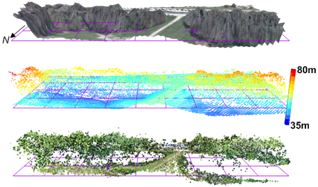
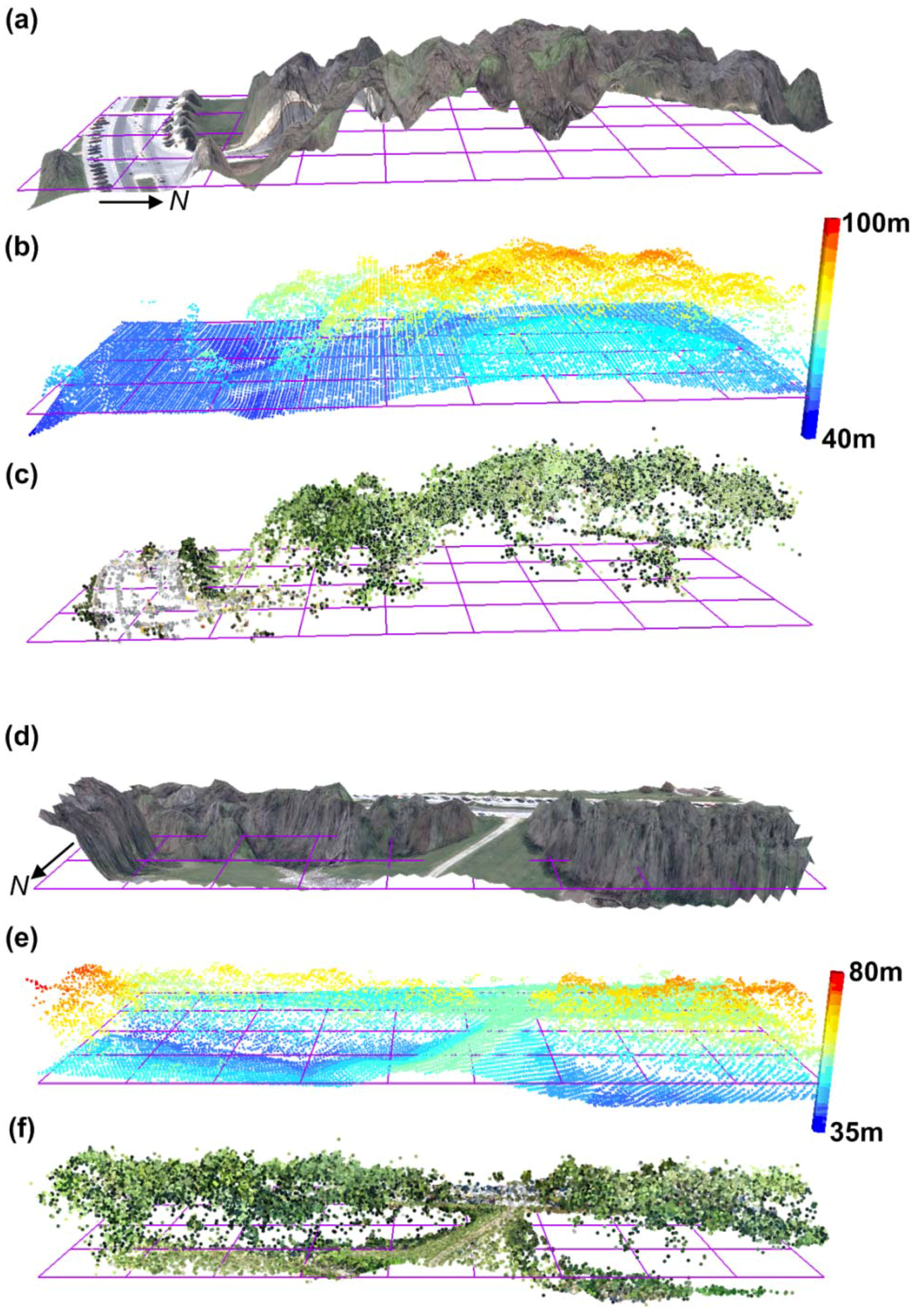
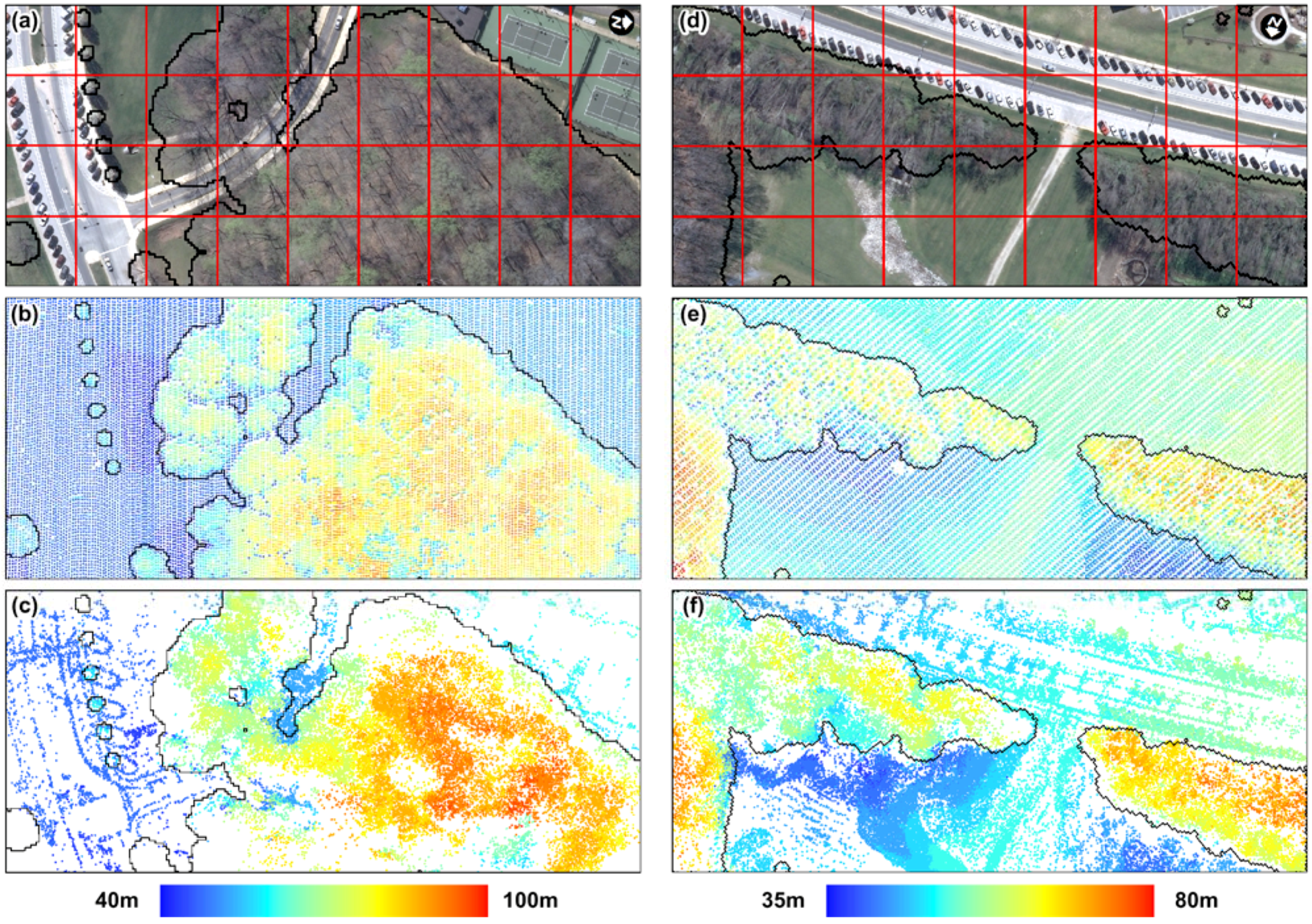
3.1. General Characteristics and Geometric Precision of Ecosynth Point Clouds
| Site | Horizontal | Vertical | ||||
|---|---|---|---|---|---|---|
| Standard | Precision | |||||
| 3 GCPs | 5 GCPs | 3 GCPs | 5 GCPs | 3 GCPs | 5 GCPs | |
| Knoll | 1.5 m | 1.0 m | 4.6 m | 4.3 m | 1.1 m | 0.9 m |
| Herbert Run | 1.1 m | 1.3 m | 6.1 m | 2.0 m | 0.6 m | 0.6 m |
| LiDAR† | 0.15 m | 0.24 m | ||||
| † Contractor reported. | ||||||
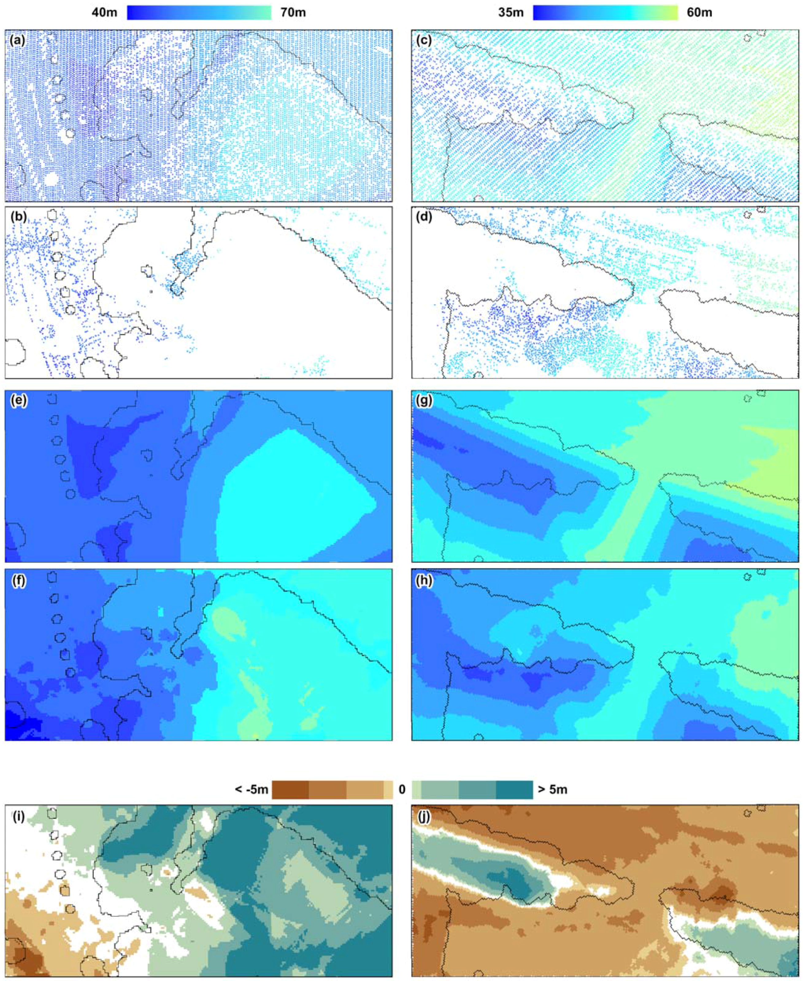
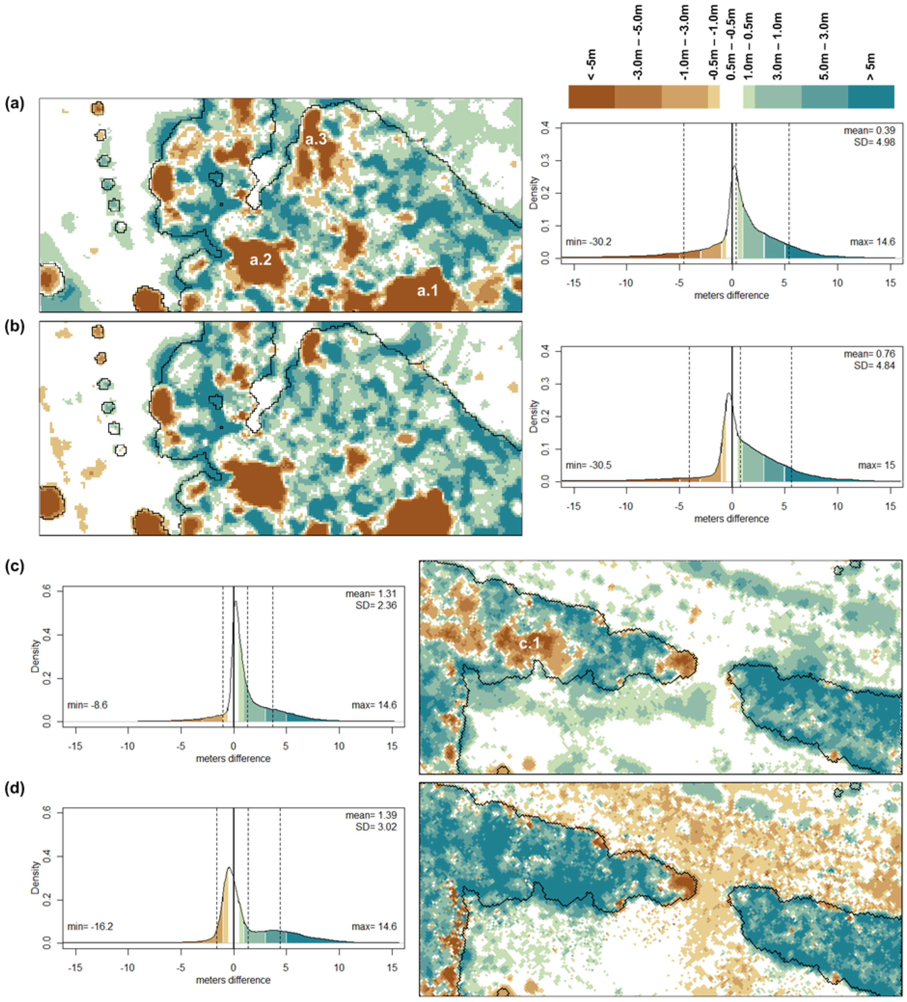
3.2. Terrain Models
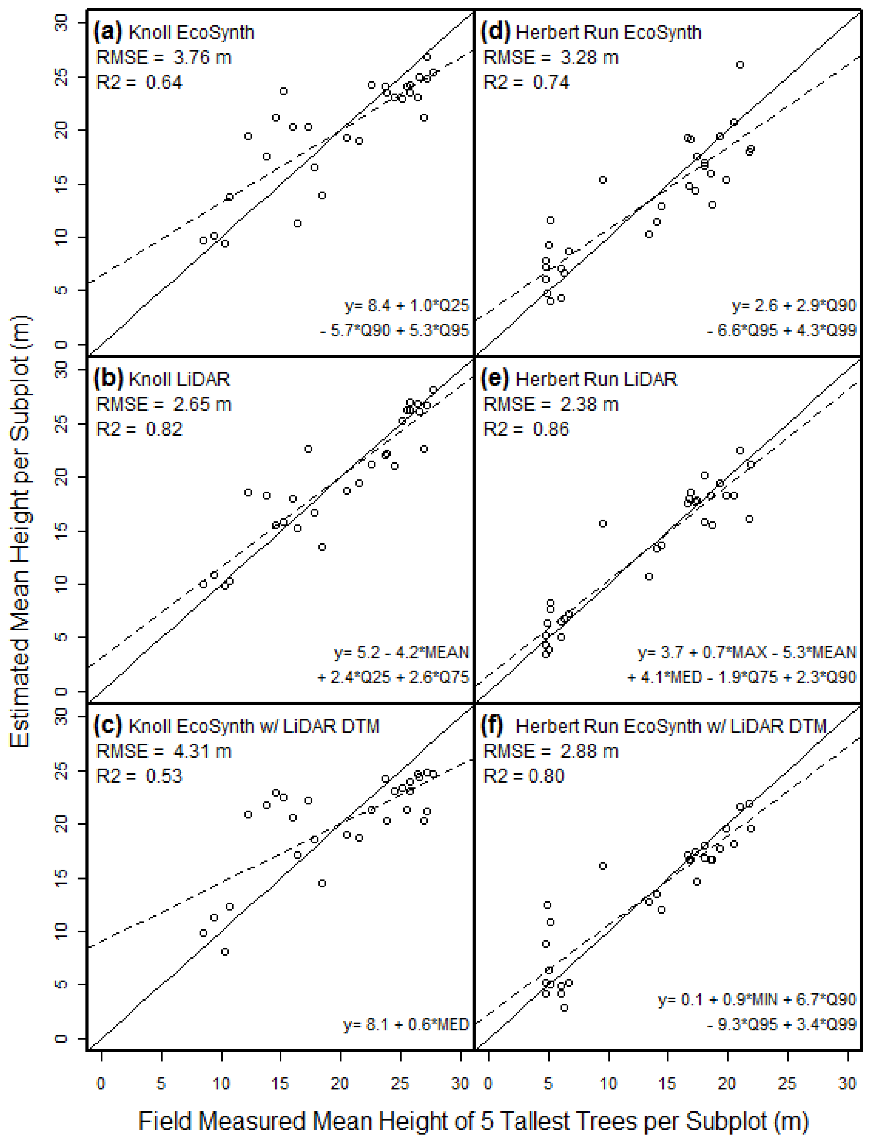
3.3. Tree Heights


3.4. Aboveground Biomass (AGB)
| Simple Linear Regression | |||
|---|---|---|---|
| Method | Equation form and metrics† | R2 | RMSE (kg AGB·m−2) |
| Standard Ecosynth | AGB = −2.0 + 1.5*Q25 | 0.41 | 12.6 |
| LiDAR | AGB = −12.0 + 2.3*Q25 | 0.60 | 10.4 |
| Precision Ecosynth + LIDAR DTM | AGB = 11.0 + 2.3*MIN | 0.37 | 13.1 |
| Multiple Linear Regression Models | |||
| Sensor | Equation form and metrics† | Adj. R2 | RMSE (kg AGB·m−2) |
| Standard Ecosynth | AGB = −0.7 + 1.7*MIN + 2.1*Q25 − 17.2*Q90 + 15.9*Q95 | 0.52 | 11.3 |
| LiDAR | AGB = −13.8 + 23.3*MEAN99 + 2.2*Q25 + 3.4*Q90 − 26.5*Q99 | 0.68 | 9.2 |
| Precision Ecosynth + LIDAR DTM | AGB = −4.6 + 1.8*MIN + 0.7*Q99 | 0.46 | 11.9 |
| † Subplot height metrics from CHMs: MEAN = mean height; MED = median height; MAX = maximum height; MIN = minimum height; MEAN99 = mean of all points > 99th quantile; Q25, Q75, Q90, Q95, Q99 = Height Quantiles. | |||
4. Conclusions
| Challenges | Solutions |
|---|---|
| Uneven point cloud coverage | |
| Accurate georeferencing |
|
| Optimal image acquisition |
|
| Poor canopy penetration |
|
| Limited spatial extent |
|
| Image processing time |
|
Acknowledgements
References and Notes
- Frolking, S.; Palace, M.W.; Clark, D.B.; Chambers, J.Q.; Shugart, H.H.; Hurtt, G.C. Forest disturbance and recovery: A general review in the context of spaceborne remote sensing of impacts on aboveground biomass and canopy structure. J. Geophys. Res. 2009, 114, G00E02:27. [Google Scholar] [CrossRef]
- Asner, G.P. Tropical forest carbon assessment: integrating satellite and airborne mapping approaches. Environ. Res. Lett. 2009, 4. [Google Scholar] [CrossRef]
- Houghton, R.A.; Hall, H.; Goetz, S.J. Importance of biomass in the global carbon cycle. J. Geophys. Res. 2009, 114, G00E03:13. [Google Scholar] [CrossRef]
- Vierling, K.T.; Vierling, L.A.; Gould, W.A.; Martinuzzi, S.; Clawges, R.M. Lidar: shedding new light on habitat characterization and modeling. Front. Ecol. Environ. 2008, 6, 90–98. [Google Scholar] [CrossRef]
- Bergen, K.M.; Goetz, S.J.; Dubayah, R.O.; Henebry, G.M.; Hunsaker, C.T.; Imhoff, M.L.; Nelson, R.F.; Parker, G.G.; Radeloff, V.V. Remote sensing of vegetation 3-D structure for biodiversity and habitat: Review and implications for LiDAR and radar spaceborne missions. J. Geophys. Res. 2009, 114, G00E06:13. [Google Scholar] [CrossRef]
- Andersen, H.E.; McGaughey, R.J.; Reutebuch, S.E. Estimating forest canopy fuel parameters using LIDAR data. Remote Sens.Environ. 2005, 94, 441–449. [Google Scholar] [CrossRef]
- Skowronski, N.; Clark, K.; Nelson, R.; Hom, J.; Patterson, M. Remotely sensed measurements of forest structure and fuel loads in the Pinelands of New Jersey. Remote Sens.Environ. 2007, 108, 123–129. [Google Scholar] [CrossRef]
- Naesset, E. Predicting forest stand characteristics with airborne scanning laser using a practical two-stage procedure and field data. Remote Sens. Environ. 2002, 80, 88–99. [Google Scholar] [CrossRef]
- Zhao, K.; Popescu, S. Lidar-based mapping of leaf area index and its use for validating GLOBCARBON satellite LAI product in a temperate forest of the southern USA. Remote Sens. Environ. 2009, 113, 1628–1645. [Google Scholar] [CrossRef]
- Lefsky, M.A.; Cohen, W.B.; Parker, G.G.; Harding, D.J. Lidar remote sensing for ecosystem studies. Bioscience 2002, 52, 20–30. [Google Scholar] [CrossRef]
- St-Onge, B.; Hu, Y.; Vega, C. Mapping the height and above-ground biomass of a mixed forest using LiDAR and stereo Ikonos images. Int. J. Remote Sens. 2008, 29, 1277–1294. [Google Scholar] [CrossRef]
- Wehr, A.; Lohr, U. Airborne laser scanning—An introduction and overview. ISPRS J. Photogramm. 1999, 54, 68–82. [Google Scholar] [CrossRef]
- Nelson, R.; Parker, G.; Hom, M. A portable airborne laser system for forest inventory. Photogramm. Eng. Remote Sens. 2003, 69, 267–273. [Google Scholar] [CrossRef]
- Rango, A.; Laliberte, A.; Herrick, J.E.; Winters, C.; Havstad, K.; Steele, C.; Browning, D. Unmanned aerial vehicle-based remote sensing for rangeland assessment, monitoring, and management. J. Appl. Remote Sens. 2009, 3, 033542:15. [Google Scholar]
- Hunt, J.; Raymond, E.; Hively, W.D.; Fujikawa, S.; Linden, D.; Daughtry, C.S.; McCarty, G. Acquisition of NIR-green-blue digital photographs from unmanned aircraft for crop monitoring. Remote Sens. 2010, 2, 290–305. [Google Scholar] [CrossRef]
- Wundram, D.; Loffler, J. High-resolution spatial analysis of mountain landscapes using a low-altitude remote sensing approach. Int. J. Remote Sens. 2008, 29, 961–974. [Google Scholar] [CrossRef]
- Snavely, N.; Seitz, D.; Szeliski, R. Modeling the world from internet photo collections. Int J. Comput. Vis. 2008, 80, 189–210. [Google Scholar] [CrossRef]
- Triggs, B.; McLauchlan, P.; Hartley, R.; Fitzgibbon, A. Bundle adjustment—A modern synthesis. In Proceedings of International ICCV Workshop on Vision Algorithms, Corfu, Greece, September 1999; Springer: Berlin/Heidelberg, Germany, 2000; Volume 1883, pp. 298–372. [Google Scholar]
- Snavely, N. Bundler—Structure from Motion for Unordered Image Collections, Version 0.4. Available online: http://phototour.cs.washington.edu/bundler/ (accessed on January 29, 2010).
- Lowe, D.G. Distinctive image features from scale-invariant keypoints. Int. J. Comput. Vis. 2004, 60, 91–110. [Google Scholar] [CrossRef]
- Lourakis, M.I.; Argyros, A.A. SBA: A software package for generic sparse bundle adjustment. ACM Trans. Math. Softw. 2009, 36. [Google Scholar] [CrossRef]
- de Matías, J.; de Sanjosé, J.J.; López-Nicolás, G.; Sagüés, C.; Guerrero, J.J. Photogrammetric methodology for the production of geomorphologic maps: Application to the Veleta Rock Glacier (Sierra Nevada, Granada, Spain). Remote Sens. 2009, 1, 829–841. [Google Scholar] [CrossRef]
- Strecha, C.; von Hansen, W.; Van Gool, L.; Thoennessen, U. Multi-view stereo and LiDAR for outdoor scene modelling. In Proceedings of the PIA07—Photogrammetric Image Analysis Conference, Munich, Germany, September 2007.International Archives of Photogrammetry, Remote Sensing and Spatial Information Sciences; Stilla, U.; Mayer, H.; Rottensteiner, F.; Heipke, C.; Hinz, S. (Eds.) Institute of Photogrammetry and Cartography: Friesland, The Netherlands, 2007.
- Photosynth. Microsoft: Photosynth. Available online: http://photosynth.net/Default.aspx (accessed on February 10, 2010).
- Dowling, T.I.; Read, A.M.; Gallant, J.C. Very high resolution DEM aquisition at low cost using a digital camera and free software. In Proceedings of the 18th World IMACS / MODSIM Congress, Cairns, Australia; 2009. [Google Scholar]
- Grzeszczuk, R.; Košecka, J.; Vedantham, R.; Hile, H. Creating Compact Architectural Models by Geo-registering Image Collections. In Proceedings of the 2009 IEEE International Workshop on 3D Digital Imaging and Modelling (3DIM 2009), Kyoto, Japan; 2009. [Google Scholar]
- CHDK. CHDK Wiki. Available online: http://chdk.wikia.com/wiki/CHDK (accessed on January 21, 2010).
- Wolf, P.R. Elements of Photogrammetry with Air Photo Interpretation and Remote Sensing; McGraw-Hill Book Company: New York, NY, USA, 1983. [Google Scholar]
- Nedler, J.A.; Mead, R. Simplex method for function minimizations. Comput. J. 1965, 7, 308–313. [Google Scholar]
- Hood, G. PopTools Version 3.1.0. Available online: http://www.cse.csiro.au/poptools/index.htm (accessed on February 10, 2010).
- USGS EROS Center. Available online: http://eros.usgs.gov/ (accessed on October 1, 2009).
- Millard, S.P.; Neerchal, N.K. Environmental Statistics with S-Plus; Applied Environmental Statistics Series; CRC Press: Boca Raton, FL, USA, 2001. [Google Scholar]
- Rousseeuw, P.J.; Leroy, A.M. Robust Regression and Outlier Detection; John Wiley: New York, NY, USA, 1987. [Google Scholar]
- Zhang, K.; Chen, S.; Whitman, D.; Shyu, M.; Yan, J.; Zhang, C. A progressive morphological filter for removing nonground measurements from airborne LiDAR data. IEEE Trans. Geosci. Remote Sens. 2003, 41, 872–882. [Google Scholar] [CrossRef]
- Zhang, K.; Cui, K. ALDPAT V1.0: Airborne LiDAR Data Processing and Analysis Tools. 2007. Available online: http://lidar.ihrc.fiu.edu/lidartool.html (accessed on February 10, 2010).
- ArcGIS Desktop; V9.3.1: Geostatistical Analyst Extension; Environmental Systems Research Institute, ESRI: Redlands, CA, USA, 2009.
- Means, J.E.; Acker, S.A.; Brandon, J.; Fritt, B.J.; Renslow, M.; Emerson, L.; Hendrix, C. Predicting forest stand characteristics with airborne scanning LiDAR. Photogramm. Eng. Remote Sensing 2000, 66, 1367–1371. [Google Scholar]
- R: A Language and Environment for Statistical Computing, V2.10.1; R Foundation for Statistical Computing: Vienna, Austria, 2009.
- Lefsky, M.A.; Harding, D.; Cohen, W.B.; Parker, G.G.; Shugart, H.H. Surface LiDAR remote sensing of basal area and biomass in deciduous forests of eastern Maryland, USA. Remote Sens. Environ. 1999, 67, 83–98. [Google Scholar] [CrossRef]
- Hurtt, G.; Dubayah, R.O.; Drake, J.B.; Moorcroft, P.; Pacala, S.; Blair, J.B.; Fearon, M. Beyond potential vegetation: combining LiDAR data and a height-structured model for carbon studies. Ecol. Appl. 2004, 14, 873–883. [Google Scholar] [CrossRef]
- Jenkins, J.C.; Chojnacky, D.C.; Health, L.S.; Birdsey, R.A. National-scale biomass estimators for United States tree species. Forest Sci. 2003, 49, 12–35. [Google Scholar]
- Lingua, A.; Marenchino, D.; Nex, F. Performance analysis of the SIFT operator for automatic feature extraction and matching in photogrammetric applications. Sensors 2009, 9, 3745–3766. [Google Scholar] [CrossRef] [PubMed]
- Sithole, G.; Vosselman, G. Experimental comparison of filter algorithms for bare-Earth extraction from airborne laser scanning point clouds. ISPRS J. Photogramm. 2004, 59, 85–101. [Google Scholar] [CrossRef]
- Drake, J.B.; Dubayah, R.O.; Clark, D.B.; Knox, R.G.; Blair, J.B.; Hofton, M.A.; Chazdon, R.L.; Weishampel, J.F.; Prince, S.D. Estimation of tropical forest structural characteristics using large-footprint LiDAR. Remote Sens. Environ. 2002, 79, 305–319. [Google Scholar] [CrossRef]
- Lefsky, M.A.; Cohen, W.B.; Harding, D.; Parker, G.G.; Acker, S.; Gower, S. LiDAR remote sensing of above-ground biomass in three biomes. Global Ecol. Biogeogr. 2002, 11, 393–399. [Google Scholar] [CrossRef]
- Furukawa, Y.; Ponce, J. Accurate, dense, and robust multi-view stereopsis. In Proceedings of International Conference on Computer Vision and Patten Recnognition, Minneapolis, MN, USA; 2007. [Google Scholar]
- Asner, G.P.; Martin, R.E. Airborne spectranomics: mapping canopy chemical and taxonomic diversity in tropical forests. Front. Ecol. Environ. 2009, 7, 269–276. [Google Scholar] [CrossRef]
- Vitousek, P.; Asner, G.P.; Chadwick, O.A.; Hotchkiss, S. Landscape-level variation in forest structure and biogeochemistry across a substrate age gradient in Hawaii. Ecology 2009, 90, 3074–3086. [Google Scholar] [CrossRef] [PubMed]
- Anderson, J.E.; Plourde, L.C.; Martin, M.E.; Braswell, B.H.; Smith, M.L.; Dubayah, R.O.; Hofton, M.A.; Blair, J.B. Integrating waveform LiDAR with hyperspectral imagery for inventory of a northern temperate forest. Remote Sens. Environ. 2008, 112, 1856–1870. [Google Scholar] [CrossRef]
- Richardson, A.D.; Braswell, B.H.; Hollinger, D.Y.; Jenkins, J.P.; Ollinger, S.V. Near-surface remote sensing of spatial and temporal variation in canopy phenology. Ecol. Appl. 2009, 19, 1417–1428. [Google Scholar] [CrossRef] [PubMed]
© 2010 by the authors; licensee MDPI, Basel, Switzerland. This article is an open-access article distributed under the terms and conditions of the Creative Commons Attribution license (http://creativecommons.org/licenses/by/3.0/).
Share and Cite
Dandois, J.P.; Ellis, E.C. Remote Sensing of Vegetation Structure Using Computer Vision. Remote Sens. 2010, 2, 1157-1176. https://doi.org/10.3390/rs2041157
Dandois JP, Ellis EC. Remote Sensing of Vegetation Structure Using Computer Vision. Remote Sensing. 2010; 2(4):1157-1176. https://doi.org/10.3390/rs2041157
Chicago/Turabian StyleDandois, Jonathan P., and Erle C. Ellis. 2010. "Remote Sensing of Vegetation Structure Using Computer Vision" Remote Sensing 2, no. 4: 1157-1176. https://doi.org/10.3390/rs2041157
APA StyleDandois, J. P., & Ellis, E. C. (2010). Remote Sensing of Vegetation Structure Using Computer Vision. Remote Sensing, 2(4), 1157-1176. https://doi.org/10.3390/rs2041157