Potential of Using Remote Sensing Techniques for Global Assessment of Water Footprint of Crops


 ,
,
Abstract
:1. Introduction
2. State of the Art
2.1. Water Footprint of Crops

- coarse spatial resolution of the source data, mainly where extracted from statistical databases,
- coarse temporal resolution of the input data, which may imply the use of interpolation techniques,
- assumption of ideal conditions, e.g., optimum soil water conditions,
- outputs are static, i.e., they are given for particular periods of time.
2.2. Irrigation Mapping
3. Methodology
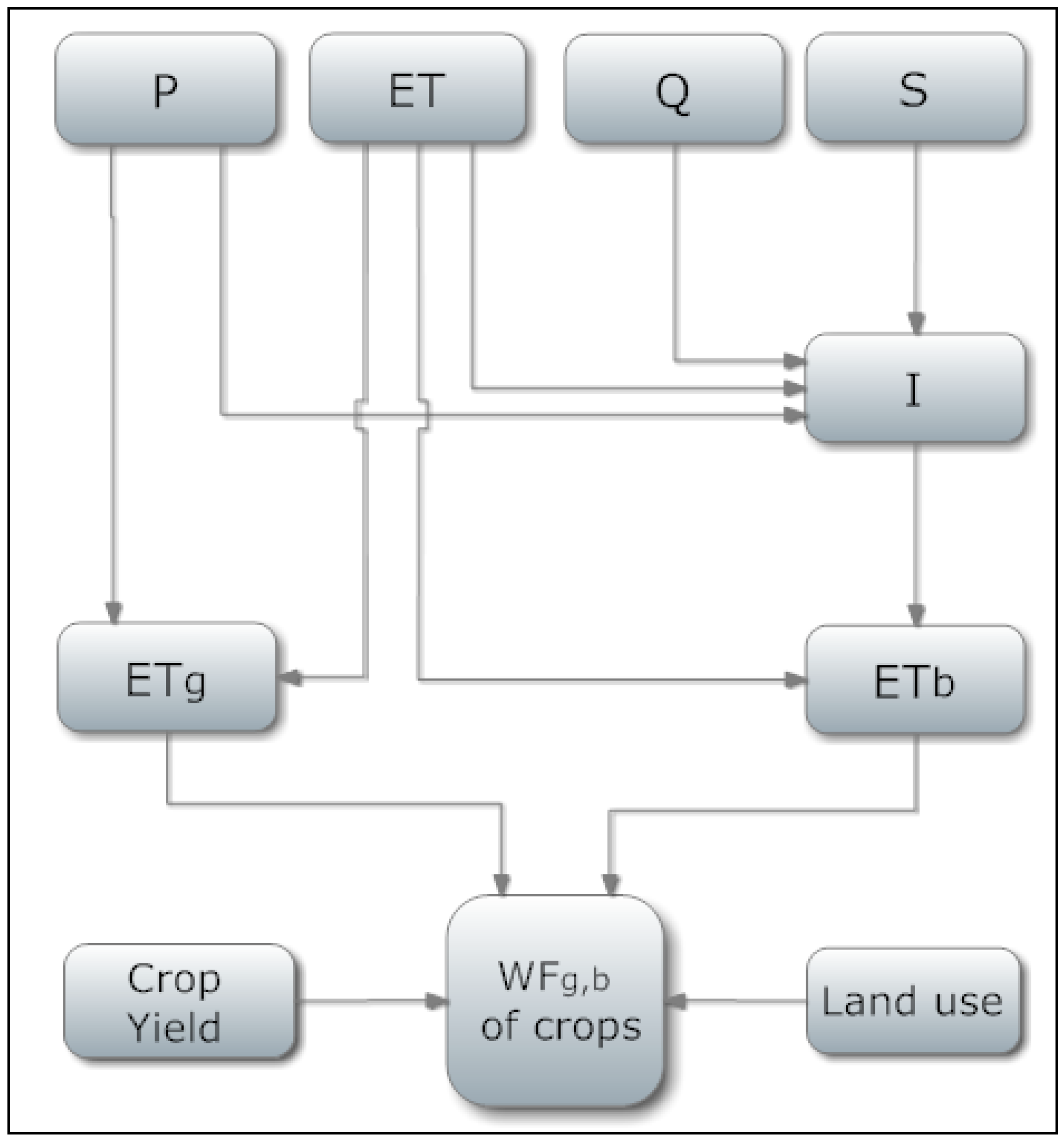
3.1. Theory

3.2. Global EO Products

| EO product | Source | Spatial coverage | Spatial resolution | Temporal resolution | Main input | Data availability |
|---|---|---|---|---|---|---|
| P | CMORPH | Global | 8 km at the equator | 30’ monthly | MW IR | 2002–present |
| PERSIANN | Global | 0.25° | 6h | IR | 2000–present | |
| MPE | Meteosat disk * | Met7:5 km at nadir | Met7: 30’ | MW IR | 2000–present | |
| Met8:3 km at nadir | Met8: 15’ | |||||
| Met9:3 km at nadir | Met9: 15’ | |||||
| ET | MET | Meteosat disk * | 3 km at nadir | 30’ | Radiation fluxes | Pre-operational (available) |
| LAI, FVC | ||||||
| Climatic data | ||||||
| MOD 16 | Global | 1 km | daily | Land cover | Pre-operational (not available) | |
| LAI, FAPAR | ||||||
| Climatic data | ||||||
| S | GRACE | Global | 400 km | monthly | Gravity fields | 2002–present |
| Q | GLDAS | Global | 1° | 3h monthly | Land cover | 1979–present |
| LAI and soil par. | ||||||
| Skin temperature | ||||||
| Radiation fluxes | ||||||
| Climatic data |
3.3. Estimation of Evapotranspiration from Remote Sensing Data
3.4. Land Use from Remote Sensing Data
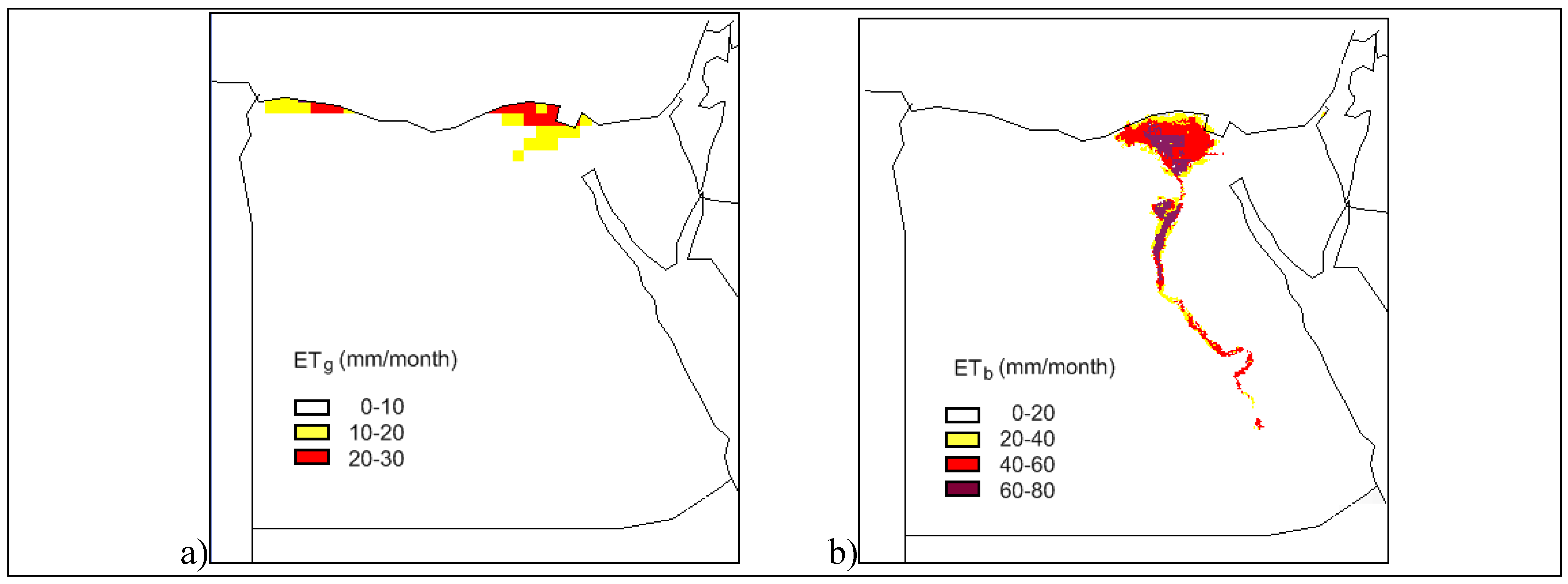
3.5. Example

| Country | Blue WF (Mm3/year) | Green WF (Mm3/year) |
|---|---|---|
| India | 81,335 | 44,025 |
| China | 47,370 | 83,459 |
| Pakistan | 27,733 | 12,083 |
| Iran | 10,940 | 26,699 |
| Egypt | 5,930 | 1,410 |
| United States | 5,503 | 111,926 |
| World | 203,744 | 760,301 |
4. Discussion
4.1. Uncertainty
4.2. Limitations
5. Conclusions
Acknowledgement
References
- Hoekstra, A.Y. Virtual water trade. In Proceedings of the International Expert Meeting on Virtual Water Trade, Value of Water Research Report Series No.12. IHE Delft, The Netherlands; 2003. [Google Scholar]
- Hoekstra, A.Y.; Chapagain, A.K. Globalization of Water. Sharing the Planet’s Freshwater Resources; Blackwell Publishing: Oxford, UK, 2008; pp. 1–208. [Google Scholar]
- Allan, J.A. Virtual water: A strategic resource global solutions to regional deficits. Ground Water 1998, 36, 545–546. [Google Scholar] [CrossRef]
- Hoekstra, A.Y.; Hung, P.Q. Globalisation of water resources: international virtual water flows in relation to crop trade. Global Environ. Change 2005, 15, 45–56. [Google Scholar] [CrossRef]
- Chapagain, A.K.; Hoekstra, A.Y. The global component of freshwater demand and supply: an assessment of virtual water flows between nations as a result of trade in agricultural and industrial products. Water Int. 2008, 33, 19–32. [Google Scholar] [CrossRef]
- Baret, F.; Hagolle, O.; Geiger, B.; Bicheron, P.; Miras, B.; Huc, M.; Berthelot, B.; Nino, F.; Weiss, M.; Samain, O.; Roujean, J.L.; Leroy, M. LAI, fAPAR and fCover CYCLOPES global products derived from VEGETATION—Part 1: Principles of the algorithm. Remote Sens. Environ. 2007, 110, 275–286. [Google Scholar] [CrossRef]
- Wagner, W.; Scipal, K. Large-scale soil moisture mapping in western Africa using the ERS scatterometer. IEEE Trans. Geosci. Remote Sens. 2000, 38, 1777–1782. [Google Scholar] [CrossRef]
- Sobrino, J.A.; Romaguera, M. Land surface temperature retrieval from MSG1-SEVIRI data. Remote Sens. Environ. 2004, 92, 247–254. [Google Scholar] [CrossRef]
- Guanter, L.; Gomez-Chova, L.; Moreno, J. Coupled retrieval of aerosol optical thickness, columnar water vapor and surface reflectance maps from ENVISAT/MERIS data over land. Remote Sens. Environ. 2008, 112, 2898–2913. [Google Scholar] [CrossRef]
- Bartholome, E.; Belward, A.S. GLC2000: A new approach to global land cover mapping from Earth observation data. Int. J. Remote Sens. 2005, 26, 1959–1977. [Google Scholar] [CrossRef]
- Joyce, R.J.; Janowiak, J.E.; Arkin, P.A.; Xie, P.P. CMORPH: A method that produces global precipitation estimates from passive microwave and infrared data at high spatial and temporal resolution. J. Hydrometeorol. 2004, 5, 487–503. [Google Scholar] [CrossRef]
- Mu, Q.; Heinsch, F.A.; Zhao, M.; Running, S.W. Development of a global evapotranspiration algorithm based on MODIS and global meteorology data. Remote Sens. Environ. 2007, 111, 519–536. [Google Scholar] [CrossRef]
- Rodell, M.; Velicogna, I.; Famiglietti, J.S. Satellite-based estimates of groundwater depletion in India. Nature 2009, 460, 999–U980. [Google Scholar] [CrossRef] [PubMed]
- Melesse, A.M.; Shih, S.F. Spatially distributed storm runoff depth estimation using Landsat images and GIS. Comput. Electron. Agric. 2002, 37, 173–183. [Google Scholar] [CrossRef]
- Liu, J.G.; Zehnder, A.J.B.; Yang, H. Global consumptive water use for crop production: The importance of green water and virtual water. Water Resour. Res. 2009, 45, 15. [Google Scholar] [CrossRef]
- Mekonnen, M.M.; Hoekstra, A.Y. A Global and High-Resolution Assessment of the Green, Blue and Grey Water Footprint of Wheat; Value of Water Research Report No.42; UNESCO-IHE: Delft, The Netherlands, 2010. [Google Scholar]
- Siebert, S.; Döll, P. Quantifying blue and green virtual water contents in global crop production as well as potential production losses without irrigation. J. Hydrol. 2010, 384, 198–217. [Google Scholar] [CrossRef]
- Hoekstra, A.Y.; Chapagain, A.K. Water footprints of nations: Water use by people as a function of their consumption pattern. Water Resour. Manag. 2007, 21, 35–48. [Google Scholar] [CrossRef]
- Hoekstra, A.Y.; Chapagain, A.K.; Aldaya, M.M.; Mekonnen, M.M. Water Footprint Manual. State of the Art 2009; Water footprint Network: Enschede, The Netherlands, 2009. [Google Scholar]
- Allen, R.; Pereira, L.S.; Raes, D.; Smith, M. FAO Irrigation and Drainage Paper No. 56: Crop Evapotranspiration; FAO in UN: Rome, Italy, 1998. [Google Scholar]
- Smith, M. CROPWAT:Manual and Guidelines; FAO in UN: Rome, Italy, 1991. [Google Scholar]
- FAO. CROPWAT 8.0 Model; Food and Agriculture Organization: Rome, Italy; Available online: www.fao.org/nr/water/infores_databases_cropwat.html (accessed on 22 April 2010).
- FAO. FAOSTAT Database; Food and Agriculture Organization: Rome, Italy; Available online: http://faostat.fao.org (accessed on 22 April 2010).
- FAO. CLIMWAT 2.0 Database; Food and Agriculture Organization: Rome, Italy; Available online: www.fao.org/nr/water/infores_databases_climwat.html (accessed on 22 April 2010).
- Portmann, F.T.; Siebert, S.; Döll, P. MIRCA2000-Global Monthly Irrigated and Rainfed Crop Areas around the year 2000: A new high-resolution data set for agricultural and hydrological modeling. Glob. Biogeochem. Cycle 2010. [Google Scholar] [CrossRef]
- Mitchell, T.D.; Jones, P.D. An improved method of constructing a database of monthly climate observations and associated high-resolution grids. Int. J. Climatol. 2005, 25, 693–712. [Google Scholar] [CrossRef]
- Liu, J.; Wiberg, D.; Zehnder, A.J.B.; Yang, H. Modeling the role of irrigation in winter wheat yield, crop water productivity, and production in China. Irrig. Sci. 2007, 26, 21–33. [Google Scholar] [CrossRef]
- Ramankutty, N.; Evan, A.T.; Monfreda, C.; Foley, J.A. Farming the planet: 1. Geographic distribution of global agricultural lands in the year 2000. Glob. Biogeochem. Cycle 2008, 22. [Google Scholar] [CrossRef]
- Portmann, F.; Siebert, S.; Bauer, C.; Döll, P. Global Data Set of Monthly Growing Areas of 26 Irrigated Crops; Institute of Physical Geography, University of Frankfurt (Main): Frankfurt, Germany, 2008. [Google Scholar]
- Batjes, N.H. ISRIC-WISE Derived Soil Properties on a 5 by 5 Arc-Minutes Global Grid; International Soil Reference & Information Centre: Wageningen, The Netherlands, 2006. [Google Scholar]
- FAO. AQUASTAT Database; Food and Agriculture Organization: Rome, Italy; Available online: www.fao.org/nr/water/aquastat/main/index.stm (accessed on 22 April 2010).
- Siebert, S.; Hoogeveen, J.; Frenken, K. Irrigation in Africa, Europe and Latin America. Update of the Digital Global Map of Irrigation Areas to Version 4; Institute of Physical Geography, University of Frankfurt (Main): Frankfurt, Germany, 2006. [Google Scholar]
- Siebert, S.; Döll, P.; Hoogeveen, J.; Faures, J.M.; Frenken, K.; Feick, S. Development and validation of the global map of irrigation areas. Hydrol. Earth Syst. Sci. 2005, 9, 535–547. [Google Scholar] [CrossRef]
- Ozdogan, M.; Gutman, G. A new methodology to map irrigated areas using multi-temporal MODIS and ancillary data: An application example in the continental US. Remote Sens. Environ. 2008, 112, 3520–3537. [Google Scholar] [CrossRef]
- Thenkabail, P.S.; Biradar, C.M.; Noojipady, P.; Dheeravath, V.; Li, Y.J.; Velpuri, M.; Gumma, M.; Gangalakunta, O.R.P.; Turral, H.; Cai, X.L.; Vithanage, J.; Schull, M.A.; Dutta, R. Global irrigated area map (GIAM), derived from remote sensing, for the end of the last millennium. Int. J. Remote Sens. 2009, 30, 3679–3733. [Google Scholar] [CrossRef]
- Hsu, K.L.; Gao, X.G.; Sorooshian, S.; Gupta, H.V. Precipitation estimation from remotely sensed information using artificial neural networks. J. Appl. Meteorol. 1997, 36, 1176–1190. [Google Scholar] [CrossRef]
- Hsu, K.-l.; Gupta, H.V.; Gao, X.; Sorooshian, S. Estimation of physical variables from multichannel remotely sensed imagery using a neural network: Application to rainfall estimation. Water Resour. Res. 1999, 35, 1605–1618. [Google Scholar] [CrossRef]
- Heinemann, T.; Latanzio, A.; Roveda, F. The Eumetsat multi-sensor precipitation estimate (MPE). In Second International Precipitation Working group (IPWG) Meeting, Madrid, Spain, September 2002.
- Gellens-Meulenberghs, F.; Arboleda, A.; Ghilain, N. Towards a continuous monitoring of evapotranspiration based on MSG data. In Proceedings of Symposium HS3007 at IUGG2007, Perugia, Italy, July 2007; IAHS Publication 316, IAHS Press: Oxfordshire, UK, 2007; p. 228. [Google Scholar]
- Swenson, S.; Wahr, J. Monitoring the water balance of Lake Victoria, East Africa, from space. J. Hydrol. 2009, 370, 163–176. [Google Scholar] [CrossRef]
- Rodell, M.; Houser, P.R.; Jambor, U.; Gottschalck, J.; Mitchell, K.; Meng, C.J.; Arsenault, K.; Cosgrove, B.; Radakovich, J.; Bosilovich, M.; Entin, J.K.; Walker, J.P.; Lohmann, D.; Toll, D. The global land data assimilation system. Bull. Amer. Meteorol. Soc. 2004, 85, 381–394. [Google Scholar] [CrossRef]
- Nijssen, B.; Schnur, R.; Lettenmaier, D.P. Global retrospective estimation of soil moisture using the variable infiltration capacity land surface model, 1980–93. J. Clim. 2001, 14, 1790–1808. [Google Scholar] [CrossRef]
- Su, Z. The Surface Energy Balance System (SEBS) for estimation of turbulent heat fluxes. Hydrol. Earth Syst. Sci. 2002, 6, 85–99. [Google Scholar] [CrossRef]
- Norman, J.M.; Kustas, W.P.; Humes, K.S. Source approach for estimating soil and vegetation energy fluxes in observations of directional radiometric surface temperature. Agric. For. Meteorol. 1995, 77, 263–293. [Google Scholar] [CrossRef]
- Bastiaanssen, W.G.M.; Menenti, M.; Feddes, R.A.; Holtslag, A.A.M. A remote sensing surface energy balance algorithm for land (SEBAL)—1. Formulation. J. Hydrol. 1998, 213, 198–212. [Google Scholar] [CrossRef]
- Roerink, G.J.; Su, Z.; Menenti, M. S-SEBI: A simple remote sensing algorithm to estimate the surface energy balance. Phys. Chem. Earth P B-Hydrol. Oceans Atmos. 2000, 25, 147–157. [Google Scholar] [CrossRef]
- Glenn, E.P.; Huete, A.R.; Nagler, P.L.; Hirschboeck, K.K.; Brown, P. Integrating remote sensing and ground methods to estimate evapotranspiration. Crit. Rev. Plant Sci. 2007, 26, 139–168. [Google Scholar] [CrossRef]
- Anderson, M.C.; Norman, J.M.; Mecikalski, J.R.; Otkin, J.A.; Kustas, W.P. A climatological study of evapotranspiration and moisture stress across the continental United States based on thermal remote sensing: 1. Model formulation. J. Geophys. Res.-Atmos. 2007, 112, 17. [Google Scholar] [CrossRef]
- French, A.N.; Jacob, F.; Anderson, M.C.; Kustas, W.P.; Timmermans, W.; Gieske, A.; Su, Z.; Su, H.; McCabe, M.F.; Li, F.; Prueger, J.; Brunsell, N. Surface energy fluxes with the Advanced Spaceborne Thermal Emission and Reflection radiometer (ASTER) at the Iowa 2002 SMACEX site (USA). Remote Sens. Environ. 2005, 99, 55–65. [Google Scholar] [CrossRef]
- Jia, L.; Su, Z.B.; van den Hurk, B.; Menenti, M.; Moene, A.; De Bruin, H.A.R.; Yrisarry, J.J.B.; Ibanez, M.; Cuesta, A. Estimation of sensible heat flux using the Surface Energy Balance System (SEBS) and ATSR measurements. Phys. Chem. Earth 2003, 28, 75–88. [Google Scholar] [CrossRef]
- van der Kwast, J.; Timmermans, W.; Gieske, A.; Su, Z.; Olioso, A.; Jia, L.; Elbers, J.; Karssenberg, D.; de Jong, S. Evaluation of the Surface Energy Balance System (SEBS) applied to ASTER imagery with flux-measurements at the SPARC 2004 site (Barrax, Spain). Hydrol. Earth Syst. Sci. 2009, 13, 1337–1347. [Google Scholar] [CrossRef]
- Sobrino, J.A.; Gomez, M.; Jimenez-Munoz, C.; Olioso, A. Application of a simple algorithm to estimate daily evapotranspiration from NOAA-AVHRR images for the Iberian Peninsula. Remote Sens. Environ. 2007, 110, 139–148. [Google Scholar] [CrossRef]
- Bastiaanssen, W.G.M.; Pelgrum, H.; Wang, J.; Ma, Y.; Moreno, J.F.; Roerink, G.J.; van der Wal, T. A remote sensing surface energy balance algorithm for land (SEBAL)—2. Validation. J. Hydrol. 1998, 213, 213–229. [Google Scholar] [CrossRef]
- Friedl, M.A.; McIver, D.K.; Hodges, J.C.F.; Zhang, X.Y.; Muchoney, D.; Strahler, A.H.; Woodcock, C.E.; Gopal, S.; Schneider, A.; Cooper, A.; Baccini, A.; Gao, F.; Schaaf, C. Global land cover mapping from MODIS: algorithms and early results. Remote Sens. Environ. 2002, 83, 287–302. [Google Scholar] [CrossRef]
- ESA. GLOBCOVER Products Description Manual v2; European Space Agency: Paris, France, 2008. [Google Scholar]
- Arino, O.; Gross, D.; Ranera, F.; Leroy, M.; Bicheron, P.; Brockman, C.; Defourny, P.; Vancutsem, C.; Achard, F.; Durieux, L.; Bourg, L.; Latham, J.; Di Gregorio, A.; Witt, R.; Herold, M.; Sambale, J.; Plummer, S. GlobCover: ESA service for Global Land Cover from MERIS. In IGARSS 2007; Barcelona, Spain, 2007; pp. 2412–2415. [Google Scholar]
- Zhang, M.W.; Zhou, Q.B.; Chen, Z.X.; Liu, J.; Zhou, Y.; Cai, C.F. Crop discrimination in Northern China with double cropping systems using Fourier analysis of time-series MODIS data. Int. J. Appl. Earth Obs. Geoinf. 2008, 10, 476–485. [Google Scholar]
- Blaes, X.; Vanhalle, L.; Defourny, P. Efficiency of crop identification based on optical and SAR image time series. Remote Sens. Environ. 2005, 96, 352–365. [Google Scholar] [CrossRef]
- Rao, N.R. Development of a crop-specific spectral library and discrimination of various agricultural crop varieties using hyperspectral imagery. Int. J. Remote Sens. 2008, 29, 131–144. [Google Scholar] [CrossRef]
- Ebert, E.E.; Janowiak, J.E.; Kidd, C. Comparison of near-real-time precipitation estimates from satellite observations and numerical models. Bull. Amer. Meteorol. Soc. 2007, 88, 47–64. [Google Scholar] [CrossRef]
- Tian, Y.; Peters-Lidard, C.D.; Choudhury, B.J.; Garcia, M. Multitemporal analysis of TRMM-based satellite precipitation products for land data assimilation applications. J. Hydrometeorol. 2007, 8, 1165–1183. [Google Scholar] [CrossRef]
- Sapiano, M.R.P.; Arkin, P.A. An intercomparison and validation of high-resolution satellite precipitation estimates with 3-Hourly gauge data. J. Hydrometeorol. 2009, 10, 149–166. [Google Scholar] [CrossRef]
- Kalma, J.D.; McVicar, T.R.; McCabe, M.F. Estimating land surface evaporation: A review of methods using remotely sensed surface temperature data. Surv. Geophys. 2008, 29, 421–469. [Google Scholar] [CrossRef]
- Liu, X.; Ditmar, P.; Siemes, C.; Slobbe, D.C.; Revtova, E.A.; Klees, R.; Riva, R.; Zhao, Q. DEOS Mass Transport model (DMT-1) based on GRACE satellite data: methodology and validation. Geophys. J. Intl. 2010. [Google Scholar] [CrossRef]
- Zaitchik, B.F.; Rodell, M.; Olivera, F. Evaluation of the Global Land Data Assimilation System using global river discharge data and a source to sink routing scheme. Water Resour. Res. 2010. [Google Scholar] [CrossRef]
- Sheffield, J.; Ferguson, C.R.; Troy, T.J.; Wood, E.F.; McCabe, M.F. Closing the terrestrial water budget from satellite remote sensing. Geophys. Res. Lett. 2009, 36, 5. [Google Scholar] [CrossRef]
- Farah, H.O. Estimation of Regional Evaporation under Different Weather Conditions from Satellite and Meteorological Data: A Case Study in the Naivasha basin, Kenya. Ph.D. Thesis, University of Twente, Enschede, The Netherlands, 2001. [Google Scholar]
- Anderson, M.C.; Norman, J.M.; Mecikalski, J.R.; Otkin, J.A.; Kustas, W.P. A climatological study of evapotranspiration and moisture stress across the continental United States based on thermal remote sensing: 2. Surface moisture climatology. J. Geophys. Res.-Atmos. 2007, 112, 13. [Google Scholar] [CrossRef]
- Dong, J.; Zhuang, D.F.; Huang, Y.H.; Fu, J.Y. Advances in multi-sensor data fusion: Algorithms and applications. Sensors 2009, 9, 7771–7784. [Google Scholar] [CrossRef] [PubMed]
- ECMWF. ERA-40: ECMWF 45-year reanalysis of the global atmosphere and surface conditions 1957–2002; ECMWF Newsletter 101; ECMWF: Reading, UK, 2004. [Google Scholar]
- ECMWF. Towards a climate data assimilation system: Status update of ERA-Interim; ECMWF Newsletter 115; ECMWF: Reading, UK, 2008. [Google Scholar]
- Barthel, R.; Sonneveld, B.; Gotzinger, J.; Keyzer, M.A.; Pande, S.; Printz, A.; Gaiser, T. Integrated assessment of groundwater resources in the Oueme basin, Benin, West Africa. Phys. Chem. Earth 2009, 34, 236–250. [Google Scholar] [CrossRef]
- Chatterjee, R.; Purohit, R.R. Estimation of replenishable groundwater resources of India and their status of utilization. Curr. Sci. 2009, 96, 1581–1591. [Google Scholar]
- Agbu, P.A.; James, M.E. The NOAA/NASA Pathfinder AVHRR Land Data Set User’s Manual; Goddard Distributed Active Archive Center, NASA, Goddard Space Flight Center: Greenbelt, MD, USA, 1994. [Google Scholar]
© 2010 by the authors; licensee MDPI, Basel, Switzerland. This article is an open-access article distributed under the terms and conditions of the Creative Commons Attribution license (http://creativecommons.org/licenses/by/3.0/).
Share and Cite
Romaguera, M.; Hoekstra, A.Y.; Su, Z.; Krol, M.S.; Salama, M.S. Potential of Using Remote Sensing Techniques for Global Assessment of Water Footprint of Crops. Remote Sens. 2010, 2, 1177-1196. https://doi.org/10.3390/rs2041177
Romaguera M, Hoekstra AY, Su Z, Krol MS, Salama MS. Potential of Using Remote Sensing Techniques for Global Assessment of Water Footprint of Crops. Remote Sensing. 2010; 2(4):1177-1196. https://doi.org/10.3390/rs2041177
Chicago/Turabian StyleRomaguera, Mireia, Arjen Y. Hoekstra, Zhongbo Su, Maarten S. Krol, and Mhd. Suhyb Salama. 2010. "Potential of Using Remote Sensing Techniques for Global Assessment of Water Footprint of Crops" Remote Sensing 2, no. 4: 1177-1196. https://doi.org/10.3390/rs2041177
APA StyleRomaguera, M., Hoekstra, A. Y., Su, Z., Krol, M. S., & Salama, M. S. (2010). Potential of Using Remote Sensing Techniques for Global Assessment of Water Footprint of Crops. Remote Sensing, 2(4), 1177-1196. https://doi.org/10.3390/rs2041177