Comparing Machine and Deep Learning Methods for the Phenology-Based Classification of Land Cover Types in the Amazon Biome Using Sentinel-1 Time Series

Abstract

The state of Amapá within the Amazon biome has a high complexity of ecosystems formed by forests, savannas, seasonally flooded vegetation, mangroves, and different land uses. The present research aimed to map the vegetation from the phenological behavior of the Sentinel-1 time series, which has the advantage of not having atmospheric interference and cloud cover. Furthermore, the study compared three different sets of images (vertical–vertical co-polarization (VV) only, vertical–horizontal cross-polarization (VH) only, and both VV and VH) and different classifiers based on deep learning (long short-term memory (LSTM), Bidirectional LSTM (Bi-LSTM), Gated Recurrent Units (GRU), Bidirectional GRU (Bi-GRU)) and machine learning (Random Forest, Extreme Gradient Boosting (XGBoost), k-Nearest Neighbors, Support Vector Machines (SVMs), and Multilayer Perceptron). The time series englobed four years (2017–2020) with a 12-day revisit, totaling 122 images for each VV and VH polarization. The methodology presented the following steps: image pre-processing, temporal filtering using the Savitsky–Golay smoothing method, collection of samples considering 17 classes, classification using different methods and polarization datasets, and accuracy analysis. The combinations of the VV and VH pooled dataset with the Bidirectional Recurrent Neuron Networks methods led to the greatest F1 scores, Bi-GRU (93.53) and Bi-LSTM (93.29), followed by the other deep learning methods, GRU (93.30) and LSTM (93.15). Among machine learning, the two methods with the highest F1-score values were SVM (92.18) and XGBoost (91.98). Therefore, phenological variations based on long Synthetic Aperture Radar (SAR) time series allow the detailed representation of land cover/land use and water dynamics.

1. Introduction

Understanding the spatial heterogeneity of the Amazonian landscape is crucial for developing and planning efficient conservation actions in one of the world’s most diverse regions [1,2]. The mapping of the diversity of forests and vegetation is the basis for research and knowledge of the dynamics and management of forest resources, where changes in vegetation cover driven by human activities profoundly affect ecosystem functioning [3,4]. Although Amazonian landscapes are often associated with forests, they comprise a wider array of ecosystems developing along climatic, edaphic, and hydrologic gradients. This biome contains “Amazonian savannas” that constitute isolated patches of open formations consisting of grassland and shrub vegetation, covering an area of 267,000 km², mainly in Brazilian and Bolivian territory (90% of the area) [5]. The forest covers 80% of the biome area, and the “Amazonian savannas” occupy only <5% [6]. In this context, the state of Amapá, located in the extreme northeast of the Amazon region, has incomparable vegetation in the Amazon biome, formed by a fragmented and complex environment with intercalation of forests, flooded forests, floodplains, savannas, and mangroves [5]. Amapá has a high percentage of well-preserved original vegetation (>95%), containing 72% of its extension within protected areas [7]. However, the distribution of protected areas is not proportional to vegetation formations, requiring an adequate monitoring system to detect human activities.

In this sense, orbital remote sensing technology is an adequate tool to obtain periodic information about a large area practically and economically, allowing the extraction of vegetation cover, ecosystem parameters, and land-cover changes. The provision of temporally continuous information by remote sensing orbital images establishes temporal signatures that describe seasonal variations and growth cycles (e.g., flowering, fruiting, leaf change, senescence, dormancy) [8,9,10]. Satellite-derived phenology overcomes the limitations of monitoring at ground level, considering a wide spatial range, repeatable over time, normalized, and without the need for extensive and costly fieldwork [11]. This phenology approach provides environmental information covering numerous areas of knowledge, such as ecology [9,12,13], climate change [14,15,16], conservation biology [17,18,19], land-use/land-cover change [20], and crop monitoring [21]. Therefore, several studies describe the phenological dynamics from remote sensing images to assess environmental changes at multiple spatial and temporal scales [22,23], increasing phenological studies exponentially [11].

The diverse ecosystems and cloud conditions make mapping Amapá’s landscape challenging. The high presence of cloud cover in the Amazon region is a limiting factor for optical imaging [24,25,26]. Consequently, the time series of Synthetic Aperture Radar (SAR) becomes the primary alternative for being free of constant atmospheric interference in tropical areas and acquiring information without interruption. In addition to transposing climatic conditions, SAR signals are sensitive to vegetation structure and biomass, crop and vegetation height, and soil moisture, providing additional information on land-cover types [27,28]. However, SAR time series have a lesser use than optical images due to the more significant presence of noise, pre-processing complexity, difficulty in interpretation, and scarcity of free data [11].

The advent of C-band Sentinel-1 (S-1) A and B sensors belonging to the European Space Agency (ESA) mission has intensified the use of SAR time series in phenological studies due to the short revisit time interval of 6 (using both sensors) or 12 days (using a sensor) and free data distribution [29,30]. The high temporal resolution of the S-1 images causes an increase in different vegetation studies: forests [31,32,33,34], temporarily flooded vegetation [35,36], salt marshes [37], urban vegetation [38], cultivated landscape with different crop types [39,40,41,42,43,44], rural and natural landscapes [45], early crop [46], and single cultivation cycle during a year such as rice [47,48,49], and wheat [50,51,52]. Moreover, many surveys use a combination of radar and optical sensor images for vegetation classification [53], integrating S-1 data with optical images, mainly from Sentinel-2 (S-2) [54,55,56] and Landsat images [57,58,59].

Time series classification algorithms use seasonal backscatter differences to individualize and detect targets. The main S-1 time series classification algorithms are the traditional methods, Machine Learning (ML) and Deep Learning (DL). Among the traditional methods, the predominant studies use techniques based on distance and similarity measures [31,32,39,43,60] and phenology metrics [33]. Several ML techniques have been applied in the phenology-based classification of land-cover types: Random Forest (RF), Support Vector Machines (SVMs), Decision Tree (DT), K-Nearest Neighbor (KNN) and Quadratic Discriminant Analysis (QDA), Extreme Gradient Boosting (XGB), Multilayer Perceptron (MLP), Adaptive Boosting (AdaBoost), and Extreme Learning Machine (ELM). Among ML models, RF is the most used in temporal classification [34,48,61,62]. Furthermore, many studies compare the different ML methods, such as SVM and RF [45]; RF, SVM, XGBoost, MLP, AdaBoost, and ELM [38]; and DT, SVM, KNN, and QDA [49].

The DL models have recently reached state-of-the-art computer vision, with wide application in remote sensing [63,64]. DL models based on the Recurrent Neural Network (RNN) are the most hopeful in classifying temporal and hyperspectral data due to their ability to detect sequential data [65,66,67]. The distinction of RNN methods compared to other approaches is to incorporate “memory” information, where data from previous inputs influence subsequent inputs and outputs. The inputs and outputs of traditional deep neural networks are independent, while in RNNs, there is a dependence along an ordinal sequence. Among the RNN methods, the primary methods in temporal correlation analysis are Long Short-Term Memory (LSTM) [68] and Gated Recurrent Units (GRU) [69].

In optical remote sensing, RNN methods have been applied in time series to distinguish crops and vegetation dynamics using different types of sensors: Moderate Resolution Imaging Spectroradiometer (MODIS) [70,71], S-2 [72], Landsat [73,74], and Pleiades VHSR images [75] and [71]. In the SAR time series, studies compare the RNN method with other approaches: RF and LSTM [41]; LSTM, Bi-LSTM, SVM, k-NN, and Normal Bayes [47]; 1D Convolutional Neural Networks (CNN), GRUs, LSTMs, and RF [46]; and GRUs and LSTMs [76].

A confluence of coastal, riverine, and terrestrial environments in the Amapá region of the eastern Amazon of Brazil results in a very diverse and dynamical landscape that has been poorly characterized. Using the high spatial and temporal S-1 time series (C band) in the vertical–vertical (VV) co-polarization and vertical–horizontal (VH) cross-polarization for the years 2017–2020, this research aimed to:

• Describe phenological patterns of land cover/land use;
• Characterize erosion/accretion changes in coastal and fluvial environments;
• Evaluate the behavior of VV-only, VH-only, and both VV and VH (VV&VH) datasets in the differentiation of land-cover/land-use features;
• Compare the behavior of five traditional machine learning models (RF, XGBoost, SVM, k-NN, and MLP) and four RNN models (LSTM, Bi-LSTM, GRU, and Bidirectional GRU (Bi-GRU)) in time-series classification;
• Produce a land-cover/land-use map for the Amapá region.

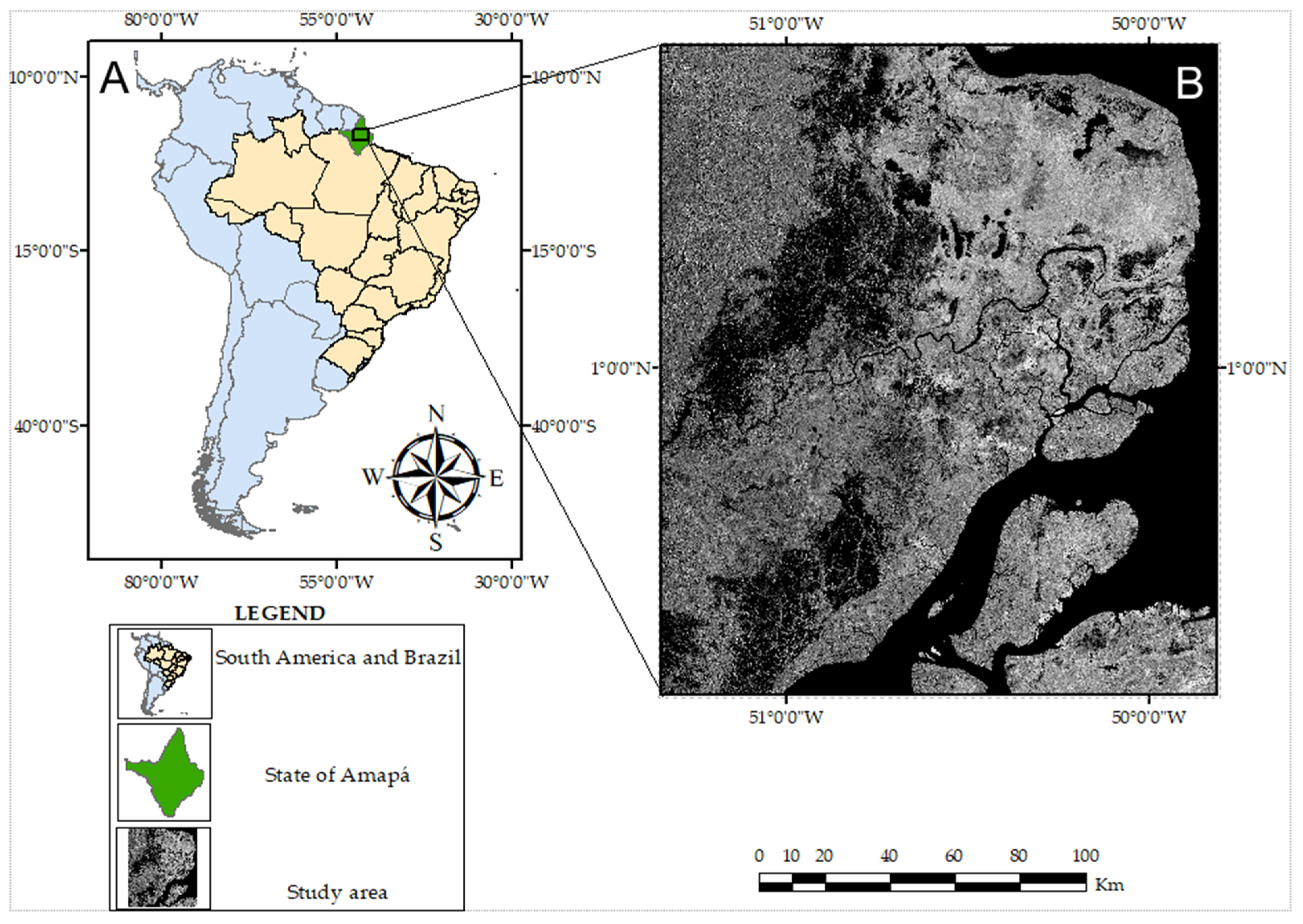
2. Study Area

The study area is located in the state of Amapá, northern Brazil (Figure 1). The climate is of type ‘Am’ in the Koppen classification, being hot and super humid with temperatures ranging from 25 to 27 °C, average monthly rainfall of 50–250 mm, and annual incidence above 2400 mm. It has two well-defined seasons: the rainy season between December and June and the dry season between July and November [77]. The vegetation of Amapá presents a significant variation from the coastal region to its interior, demarcating three main environments: coastal plain with pioneer vegetation, low plateaus with the presence of savannas, and plateau regions with rainforest cover.

The coastal plain of Amapá, with a low topographic gradient and altitude (up to 10 m), has a varied landscape composed of fluvial, fluvial-lacustrine, and fluvial-marine processes. The three predominant types of mangroves are Avicennia germinans, Rhizophora mangle, and Laguncularia racemose [78]. The Avicennia germinans is dominant in extensive areas, and more frequent in elevated, less inundated areas and under more saline conditions [79], containing the highest mangroves on the Amapá coast and forming mature and open forests [78]. Mangroves (Rhizophora spp.) are dominant in estuaries and on the inner edges of the coastal fringes, associated with rainwater [78,80]. The mangroves are interrupted by floodplain vegetation influenced by the river discharge [81].

In addition, the coastal plain of Amapá contains lakes of varying sizes and extensive seasonally flooded areas. The lakes are ox-bow-shaped, showing their evolution from abandoned meanders and past river systems [82,83]. The plain has many paleochannels, whose scars show this environment’s high dynamics and reworking [84]. Therefore, the vegetation develops in pedologically unstable areas, subjected to fluvial, lacustrine, marine, and fluviomarine accumulation processes, formed by plants adapted to local ecological conditions. The vegetation types are seasonally flooded grasses and pioneer herbaceous, shrub, and forest formations. Floodplains, along with grasslands, are the most fire-sensitive phytophysiognomies.

Savannas are present in slightly higher areas in the low plateaus of Amapá. Compared with other Amazon savannas, the savannas of Amapá showed a greater richness of genera and species with a reduced number of threatened, invasive, and exotic species [85]. The herbaceous/subshrub layer corresponded to 62% of the surveyed species [85]. The high variation in the proportions of woody and grassy plant strata provided different nomenclatures and classifications for the savannas [78,86,87,88], including the main classes: typical savanna/shrub savanna, shrub grassland (savanna parkland), and floodplain grassland (várzea). Moreover, this region is under increasing pressure from large-scale economic projects, mainly from planted forests (Eucalyptus and Acacia) [89] and soy crops using mechanized technology [90]. The savanna region (10,021 km²) contains only 917.69 km² (9.2%) of legally protected areas and 40.24 km² (0.4%) of “strictly protected” areas [91]. Nevertheless, the protected areas are predominantly “multiple uses,” allowing for various activities such as small-scale livestock farming. The region has increased the frequency of anthropic fires that threaten the quality of habitats [91,92]. Therefore, the Amazon savannas need greater surveillance and conservation plans, as they are little known, have high exposure to human occupation, and are unprotected [5].

The ecological regions of dense ombrophylous forests are predominant in the state of Amapá, occurring in the plateau regions. In the study area, forests can be lowland or submontane (less than 600 m high) with uniform canopy or emergent species (e.g., Minquartia sp., Eschweilera sp., Couma sp., and lryanthera sp.) [88].

3. Materials and Methods

The methodological framework of this study consisted of the following steps (Figure 2): (a) acquisition of the S-1 time series (10 m resolution); (b) data pre-processing; (d) noise minimization using the Savitsky–Golay smoothing filter; (e) analysis of the phenological behavior of Amazonian vegetation and human use (forest, savannah, mangrove, lowland vegetation, eucalyptus reforestation, and plantation areas); (f) comparison of classification methods (LSTM, Bi-LSTM, GRU, Bi-GRU, SVM, RF, k-NN, and MLP); and (g) accuracy analysis.

3.1. Data Preparation

The present study used an S-1 time series (C band-5.4 GHz) in the VH and VV polarizations over four years (2017 and 2020) provided by the ESA (https://scihub.copernicus.eu/dhus/#/home (accessed on 1 September 2021). The study area covers the eastern part of the state of Amapá, requiring the mosaic of two S-1 scenes from the Ground Range Detected (GRD) product in Interferometric Wide Swath mode, with a resolution of 10 × 10 m, a scene width of 250 km, and a 12-day revisit cycle [93].

The research considered 122 temporal mosaics for each polarization from 3 January 2017 to 25 December 2020, totaling four years of vegetation observation with a revisit period of 12 days. The broad temporal interval allows the detection of natural vegetation phenological cycles, flood areas, or land-use changes [94]. The image pre-processing consisted of the following steps using the Sentinel Application Platform (SNAP) software [95]: (a) apply orbital file, (b) thermal noise removal, (c) border noise removal, (d) calibration by converting digital pixel values into radiometrically calibrated SAR backscatter, (e) range-Doppler terrain correction from the Shuttle Radar Topography Mission (SRTM) digital terrain model; and (f) and linear conversion to decibels (dB). Finally, the stacking of pre-processed images generated a time cube containing the first image from 2017 to the last image from 2020. The geographic coordinates of the temporal cube are on the “x” (lines) and “y” (columns) axes, and the temporal signature is the “z” axis.

SAR images inherently have Speckle noise which causes a grainy texture of light and dark pixels, making it difficult to detect targets, especially in low-contrast areas. Noise filtering in radar images is a standard requirement, and different methods have been proposed, considering the spatial and temporal attributes of the images. In filtering time series of satellite images, a widely used method is the Savitzky and Golay (S-G) filter [96], applied to optical [97,98] and radar images [47,99,100]. The S-G filtering used a one-dimensional window size of 13 over time, allowing a smoothing of the temporal trajectory and conserving the maximum and minimum values, which are crucial for phenological analysis. Figure 3 demonstrates the effect of the S-G filter in eliminating speckles in the S-1 time series. An advantage of the S-G filter for areas with vegetation and periodic flooding is its ability to combine noise elimination and preserve phenological attributes (height, shape, and asymmetry) [101,102]. Geng et al. [103] compared eight filtering techniques for reconstructing the Normalized Difference Vegetation Index (NDVI) time series from multi-satellite sensors and showed that the S-G filter performs best in most situations. This method establishes a temporal signature that eliminates minor interferences but maintains minimum and maximum values resulting from flood events and is present in the phenology of vegetation and crops.

3.2. Ground Truth and Sample Dataset

The selections of the sample sets of temporal signatures considered the following information: (a) visual interpretation of points with a similar pattern from high-resolution Google Earth images, (b) spatial analysis of the distribution of similar temporal signatures employing the Minimum Noise Fraction transformation and end-member analysis, (c) previous information from the vegetation and land-use maps at a 1:250,000 scale developed by the Brazilian Institute of Geography and Statistics (IBGE) in 2004 [104,105], and (d) specific surveys for soybean plantations and forest plantations limited to some regions [89,90]. The IBGE mapping has a regional scale, and the land-use information referring to 2004 is outdated due to recent agricultural growth. Therefore, regional information from the IBGE mapping was a guide for the manual interpretation of the sampling points. The study disregarded areas of the city due to the use of masks.

The present time-series mapping considered the water bodies, erosion/accretion changes in coastal and river environments, and phenological patterns of land cover/land use. Therefore, seven large land-use/cover classes were subdivided into 17 subclasses according to the presence of temporal differences: water bodies (one class encompassing rivers, lakes, reservoirs, and ocean), hydrological changes (two classes including erosion and accretion areas), seasonally flooded grassland (four classes including sparse seasonally flooded grassland, dense seasonally flooded grasslands 1 and 2, and floodplain areas), pioneer formations (three classes including herbaceous, shrub, and arboreal formations), savanna (two classes including shrub grassland and savanna/shrub savanna), grassland, forest (two classes), and mangroves.

The sample selection totaled 8500 pixels (temporal signatures), well distributed, systematic, and stratified [106,107] among the 17 classes, each with 500 samples (Figure 4). Therefore, the number of samples selected for each stratum (i.e., classes or categories) was 500. The training/validation/test split [108,109] had a total of 5950 pixel samples for training (70%), 1700 pixel samples for validation (20%), and 850 pixel samples for testing (10%).

3.3. Image Classification

This study compared two broad sets of classification methods: ML versus RNN. ML methods have historically played a valuable role in remote sensing image classification and segmentation studies. However, different DL methods have outperformed traditional models with considerable improvements, having a high potential for use in land-use/land-cover classification based on temporal data.

3.3.1. Traditional Machine Learning Methods

This study tested traditional ML methods: RF [110], XGBoost [111], SVM [112], MLP [113], and k-NN [114]. The model optimization for ML and DL presents different peculiarities. The ML models usually present more easily adjustable parameters than robust models such as the LSTM or CNNs. Thus, a better way to adjust the parameters is by using a grid search. To maintain cohesion with the DL models, we used the grid search performing tests in the validation set, aiming to optimize the F-score metric.

Table 1. Configuration of the Recurrent Neural Network (RNN) models, pertaining to Deep Learning (DL) procedures, and grid search values used for each Machine Learning (ML) model: Random Forest (RF), Extreme Gradient Boosting (XGBoost), Support Vector Machines (SVMs), Multilayer Perceptron (MLP), and k-Nearest Neighbors (k-NNs).

Model		Parameter	Values
ML	RF	bootstrap	True, False
		oob_score	True, False
		max_depth	3, 5, 7
		n_estimators	50, 100, 200, 400
		min_samples_split	2, 3, 5
		max_leaf_nodes	None, 2, 4
	XGBoost	Learning_rate	0.01, 0.05, 0.1
		Min_child_weight	1, 3, 5, 7
		gamma	1, 3, 5, 7
		Colsample_bytree	0.4, 0.5, 0.6
		Max_depth	3, 5, 7
		Reg_alpha	0, 0.2, 0.3
		Subsample	0.6, 0.8
	SVM	C	0.5, 1, 2, 3, 5
		Degree	2, 3, 4
		Kernel	linear, rbf, poly
	MLP	Hidden_layer_sizes	(100,50), (200,100), (300,150)
		activation	logistic, relu, tanh
		Learning_rate	0.01, 0.001
		Max_iter	500, 1000
	k-NN	N_neighbors	5, 10, 15, 20
		Weights	uniform, distance
DL	RNN models	Epochs	5000
		Dropout	0.5
		Optimizer	Adam
		Learning rate	0.001
		Loss function	Categorical cross-entropy
		Batch size	1024
		Hidden layers	2
		Hidden layer sizes	(366, 122)

lists the grid search values used for each model. All ML models used the scikit-learn library.

3.3.2. Recurrent Neural Network Architectures

The RNN architectures are artificial intelligence methods developed for processing order-dependent data and support the use of high-dimensional input data, having a growing application in different types of studies such as natural language, audio, and video processing [115,116,117]. The two most widespread RNN methods are the LSTM [68] and the GRU [69].

The LSTM is one of the most common RNN architectures with internal memory and multiplicative gates that allow high performance on sequential data by recursively connecting sequences of information and capturing long temporal dependencies [118]. The LSTM architecture contains an input vector (Xt), current block memory (Ct), and current block output (ht), where nonlinearity activation functions are Sigmoid (σ) and hyperbolic tangent (tanh), and the vector operations are element-wise multiplication (x) and element-wise concatenation (+). Finally, the memory and output from the previous block are Ct-1 and ht-1. Among the proposed improvements to the LSTM architecture, the Bidirectional LSTM (Bi-LSTM) [119] stands out for overcoming the traditional LSTM problem of having a unidirectional strategy capable of capturing only information from previous time steps. Bi-LSTM models consider a backward layer (moving in the left-back direction) and forward layer (moving in the right-forward direction) in ordered data to capture past and future information, which makes the method more robust and contrasting with unidirectional LSTM models [120].

The GRU presents a similar structure to the LSTM models. Nonetheless, it only shows two gates in its structure, the reset and update gates. Therefore, GRU achieves a performance equivalent to LSTM but with a reduced number of ports and, consequently, fewer parameters [121]. Table 1 lists the configuration of the RNN models.

3.4. Accuracy Assessment

The accuracy comparison of the ML and DL methods considered pixel-based metrics from the confusion matrix, which yields four possibilities: true positives, true negatives, false positives, and false negatives. The accuracy analysis considered the following metrics:

$$Overall Accuracy=\frac{TP+TN}{TP+TN+FP+FN}$$

(1)

$$Precision=\frac{TP}{TP+FP},$$

(2)

$$Recall=\frac{TP}{TP+FN},$$

(3)

$$F-score=\frac{2\times \left(Precision\times Recall\right)}{Precision+Recall}.$$

(4)

Moreover, we used McNemar’s test [122] to compare the statistical differences between the two classifiers. This paired nonparametric test considers a 2 × 2 contingency table and a Chi-Squared distribution of 1 degree of freedom. The method checks whether the proportion of errors between two classifiers coincides [123].

4. Results

4.1. Temporal Backscattering Signatures

This section describes the temporal signatures of water bodies, erosion/accretion changes in the coastal and river environment, and vegetation phenological patterns. The temporal signature graphs consist of the mean value of the 500 samples selected for each target with their respective standard deviation bars. The extreme backscattering values refer to the water class with the lowest values over the period and the forest with the highest values (Figure 5). Among the intermediate values, the savannas present temporal signatures with high variation and seasonal amplitude among the natural vegetation (Figure 5).

4.1.1. Water Bodies and Accretion/Erosion Changes due to Coastal and River Dynamics

The water bodies (areas with a permanent presence of water, including oceans, seas, lakes, rivers, and reservoirs) show backscattering differences between the VV and VH polarizations due to environmental conditions and wave interference from winds and rain (Figure 5). The VV polarization is more sensitive to roughening of the water surface than VH polarization, increasing the backscatter return to the satellite. Therefore, lower VV backscatter values occur in environments under calm wind conditions (e.g., tank water and oxbow lake), while in areas with flowing water (e.g., flood water, river water, and oceans), they have higher values [124,125].

Some areas along the coast and rivers show temporal backscattering signatures that evidence transitions between terrestrial environments and areas covered by water. The temporal variation of backscatter from higher to lower values indicates erosion and progressive flooding, while the inverse indicates terrestrial accretion (Figure 6). The massive discharge of fine grains at the mouth of the Amazon River intensely influences the coastal region of the State of Amapá, presenting a high dynamic of hydrodynamic and sedimentary processes that cause a constant alteration of the coast. In the short period of analysis, the migration of mud banks from the Amazon River along the coast presented successive and recurrent phases of erosion (Figure 7A) and accretion (Figure 7B) that marked apparent changes in a few years. In addition to changes in coastline, the time series show the fluvial dynamics of active meandering rivers, evidencing the process of erosion and deposition on the banks (Figure 7C). Changes in river morphology show a progressive development over time, and it is possible to observe channels in different phases of migration and sinuosity through S-1 images.

4.1.2. Phenological Patterns

The different vegetation covers show temporal variations of backscattering (VV and VH) in the period 2017–2020, which are diagnostics for their individualization. The temporal signatures vary in floodable and non-flooded environments and different proportions of herbaceous and woody vegetation.

The interaction of C-band microwave energy in herbaceous wetlands depends on biophysical characteristics such as height, density, and canopy cover. In seasonally flooded areas, the rise in water level gradually eliminates dispersions from the soil surface and the herbaceous stratum canopy, causing microwave energy to acquire specular reflection (mirror-like reflection) from the water surfaces and decrease the backscatter values. Figure 8A,C show the seasonally flooded grassland (blue line) consisting of open areas formed predominantly by sparse herbaceous formations with periodic flooding and moist soils. Flooding over short grasslands causes the lowest backscatter values, providing the SAR time series with greater amplitudes. The grasslands covered by water during the flood season cause a specular behavior that results in a drop in backscatter values (Figure 8A,C, blue line). With the retreat of the hydrological pulse, the interaction of microwaves with the vegetation cover gradually increases and, consequently, the value of sigma naught (σ⁰). These flooded vegetation time series differ from non-floodable grassland (Figure 8A,C, red line), which present maximum backscatter values in the rainy season due to increased biomass. Therefore, there is an entirely antagonistic behavior between non-floodable savanna areas and seasonally flooded grasslands, where the peak of the backscatter values occurs at the lowest values of the other.

Seasonally flooded vegetation composed of medium and dense herbaceous vegetation causes multiple-path scattering with higher backscatter values and lower amplitude in the time series (Figure 8B,D, green and black lines). However, these grasslands show the exact dates of relative minimums during the flood period. In contrast, dense herbaceous vegetation with a sparse presence of woody vegetation (shrubs and trees) (Figure 8A, orange line) shows a change in VV polarization, which tends to have more significant canopy scattering, and the water surface portion leads to double-bounce scattering with the trunks. This behavior changes the dates with minimum values for VV polarization that tend to place them near the savanna vegetation (red line). This vegetation (Figure 8A, orange line) occurs in floodplain areas (várzea) following the drainages and intertwining with riparian forests in savannah areas, along humid dense grassland, and lake margins in the coastal plain.

The non-floodable grasslands and savannas present backscatter time series with similar formats that differ in absolute values and relative amplitude. As the tree-shrub components increase, the backscatter values increase, and the relative amplitude decreases. Figure 9A,E exemplify the increase in the proportion of arboreal vegetation in the pioneer formations: herbaceous (magenta line), shrub (yellow line), and arboreal (green line). In addition, Figure 9B,F present the time series of the shrub grassland (dark purple line) and savanna/shrub savanna (light purple line). The lowest features in the time series reflect the period of lowest precipitation, while the highest values reflect the rainy season.

Forest formations show the highest values of backscattering and low seasonal variations between the time series (Figure 9C,G), represented by ombrophilous forests in plateaus (sea-green lines) and mangroves in the coastal plain (forehead line). The representations of the ombrophilous forests considered two curves, one predominant in the study area (sea green line) and another restricted to places with the topographic effect that generate high values of backscatter (green line).

Finally, Figure 9D,H present the time series of anthropic use referring to agricultural cultivation areas (predominantly soy plantations) (blue line) and eucalyptus plantations (green line). The time series of soybean planting areas present similar shapes to savanna areas but with more accentuated minimum and maximum values of backscattering provided by anthropic activities.

4.2. Comparison between RNN and Machine Learning Methods

Table 2. Overall Accuracy (OA), precision (P), recall (R), and F-score (F1) metrics for the following methods: Deep Learning (DL), Machine Learning (ML), Long Short-Term Memory (LSTM), Bidirectional LSTM (Bi-LSTM), Gated Recurrent Unit (GRU), Bidirectional GRU (Bi-GRU), Multilayer Perceptron (MLP), Extreme Gradient Boosting (XGBoost), Random Forest (RF), Support Vector Machines (SVMs), and k-Nearest Neighbors (k-NNs). The numbers in bold represent the greatest accuracy metrics among the methods and datasets.

Model		VV				VH				VV&VH
		AO	P	R	F1	AO	P	R	F1	AO	P	R	F1
DL	Bi-GRU	85.57	85.88	85.57	85.72	91.61	91.64	91.61	91.63	93.49	93.58	93.49	93.53
	GRU	85.1	85.21	85.1	85.15	90.51	90.73	90.51	90.62	93.18	93.34	93.18	93.3
	Bi-LSTM	85.57	85.79	85.57	85.68	90.98	91.19	90.98	91.08	93.26	93.33	93.26	93.29
	LSTM	85.02	85.23	85.02	85.12	90.59	90.63	90.59	90.61	93.1	93.19	93.1	93.15
ML	RF	81.33	82.26	81.33	81.79	87.53	87.79	87.23	87.66	90.67	90.94	90.67	90.8
	XGBoost	83.14	83.99	83.14	83.56	88.39	88.63	88.39	88.51	91.92	92.04	91.92	91.98
	SVM	82.59	83.21	82.59	82.9	90.19	90.31	90.2	90.25	92.16	92.21	92.16	92.18
	k-NN	78.75	80.43	78.75	79.58	85.33	86.22	85.33	85.77	88.94	88.25	88.94	89.37
	MLP	83.77	84.1	83.77	83.93	88.78	89.81	88.78	89.29	90.82	91.2	90.82	91.01

lists the accuracy metrics for different datasets (VV-only, VH-only, and VV&VH polarizations) and classification methods. Among the datasets, the accuracy metrics show a marked difference with the following ordering: VV&VH > VH-only > VV-only. The differences in accuracy metrics between VV-only and VH-only are more remarkable than between VH-only and VV&VH. The k-NN model that obtained the smallest accuracy values in the VH-only dataset corresponded to the Bi-GRU accuracy with the greatest accuracy values in the VV-only dataset.

The Bi-GRU model presented the highest overall accuracy, precision, recall, and F-score for all three data sets (Table 2). Despite Bi-GRU being the most accurate model, the differences were not prominent with the other RNN methods, being less than 1% in the F-score. The general behavior was Bi-GRU > Bi-LSTM > GRU > LSTM, where bidirectional layers benefit the results. The SVM and the MLP obtained the highest accuracies among the ML models. Specifically, for the VH and VV&VH datasets, the SVM obtained values slightly over 1% worse than the Bi-GRU. The k-NN model obtained the worst results for all datasets, followed by the RF. The accuracy metrics between classifiers (ML or DL) show smaller differences assuming the VV&VH dataset than when applied to the VV-only and VH-only datasets. Therefore, the VV&VH dataset achieves more accurate results across all models and approximates their values.

Table 3. Per category metrics for the most accurate model Bidirectional Gated Recurrent Units (Bi-GRU) considering precision, recall, and F-score. The numbers in bold represent the greatest accuracy metrics by class, where asterisks represent equal values in different datasets.

	VV			VH			VV + VH
Class	P	R	F-Score	P	R	F-Score	P	R	F-Score
1–Water bodies	100 *	94.67	97.26	100 *	96	97.96	100 *	97.33	98.65
2–Land erosion	91.14	96	93.51	92.41	97.33	94.81	92.50	98.67	95.48
3–Land accretion	95.95	94.67	95.3	98.65	97.33	97.99	98.63	96.00	97.30
4–Sparse seasonally flooded grassland	78.16	90.67	83.95	93.51	96.00 *	94.74	96.00	96.00 *	96.00
5–Dense seasonally flooded grassland 1	87.5	84.00	85.71	94.81	97.33 *	96.05	97.33	97.33 *	97.33
6–Dense seasonally flooded grassland 2	95.89	93.33	94.59	97.30 *	96.00 *	96.64*	97.30 *	96.00 *	96.64 *
7–Dense humid grassland and floodplain areas	86.44	68.00	76.12	93.33	93.33	93.33	93.59	97.33	95.42
8–Pioneer herbaceous formation	85.9	89.33	87.58	97.22	93.33	95.24	96.00	96.00	96.00
9–Pioneer shrub formation	84.42	86.67	85.53	97.26	94.67	95.95	94.44	90.67	92.52
10–Pioneer arboreal formation	71.25	76.00	73.55	85.9	89.33	87.58	91.55	86.67	89.04
11–Shrub grassland	75.68	74.67	75.17	83.75	89.33	86.45	87.32	82.67	84.93
12–Savanna/shrub savanna	88.31	90.67	89.47	93.67	98.67	96.1	92.59	100	96.15
13–Mangroves	92.00	92.00	92.00	76.71	74.67	75.68	91.03	94.67	92.81
14–Forest 1	78.48	82.67	80.52	88.31	90.67	89.47	95.65	88.00	91.67
15–Forest 2	72.41	84.00	77.78	83.56	81.33	82.43	84.81	89.33	87.01
16–Agriculture plantations (soybean)	94.44	90.67	92.52	95.83	92.00	93.88	97.22	93.33	95.24
17–Planted forest	81.97	66.67	73.53	85.71	80.00	82.76	84.81	89.33	87.01

shows the Bi-GRU model’s accuracy metrics per land-cover/land-use category. Most classes obtained greater accuracy using the VV&VH dataset, where all categories had an F-score above 80% and 13 above 90%. In contrast, the VH dataset had 11 categories with an F-score > 90%, while the VV dataset had only six categories. This result demonstrates the complementarity of the two polarizations in the classification process. The water bodies class presented 100% accuracy, the target with the greatest accuracy in all datasets. Mangroves were the only class that obtained accuracy metrics lower than 80% for the VH-only dataset, which contrasted with the values above 90% obtained with the VV-only dataset. Additionally, mangrove precision was the only metric in which the VV-only data outperformed the other datasets. The lowest F-score with the VV&VH dataset came from the shrub grassland class (84.93%) due to confusion with other grasslands.

Figure 10 shows McNemar’s test results with a significance level of 0.05 between the paired classifications, considering nine classifiers and three datasets, totaling 27 models. Therefore, the total number of paired tests was 351, in which the colors of the grid in Figure 10 show the two hypotheses: null hypothesis (green color) and alternative hypothesis (magenta color). The null hypothesis demonstrates that the average of paired samples is equal without significant change and that the classifiers have the same proportion of errors. On the other hand, rejecting the null hypothesis demonstrates that the averages of paired samples are different with significant change.

The results demonstrate that the deep learning models are equivalent to each other within the same dataset (VV-only, VH-only, and VV&VH), given that the differences are small. Among ML methods, the SVM presented similarities to the RNN models within all datasets. In addition, two other ML methods were statistically equivalent to RNN methods within the same dataset: (a) MLP with the VV-only dataset and (b) XGBoost with the VV&VH dataset. Comparing the McNemar test between the methods with different datasets, the k-NN with the VH-only dataset had a similar result to the RNN methods using the VV-only dataset. Therefore, the least accurate method of the VH-only dataset presents statistical similarity with the best methods with the VV-only dataset. Accuracy measurements also corroborate this result. Among the VH-only and VV&VH datasets, many machine learning methods are statistically related to RNNs with VH-only.

4.3. Land-Cover/Land-Use Map

Figure 11 presents the detailed classification of an area with the highest and lowest accuracy metrics between the RNN (Bi-GRU and LSTM) and ML (SVM and k-NN) methods using the different datasets (VV only, VH only, and VV&VH). The results demonstrate a high similarity between the methods with small punctual changes, which explains the values close to the accuracy metrics.

Figure 12 presents the vegetation map of the southeastern region of the State of Amapá using the most accurate model, assuming the Bi-GRU method and the VV&VH dataset. The map shows the variation from the coastal zone to the interior with a progressive change according to topographic altitude. Along the maritime coast, the coastline has high dynamics with the presence of eroded and accretion areas. In the northeastern part of the study area, significant areas of mangroves develop along the coastal zones. The high fluvial dynamics in the coastal plain describe extensive areas with periodic flooding characterized by phenological behaviors, with minimum points in the rainy seasons and elevation of the water level (marked in cyan on the map). In the coastal plains, the high dynamics of the fluvial, fluvial-lacustrine, and fluvial-marine processes establish the formation of large lagoons and pedologically unstable areas covered by pioneer vegetation (first occupation of edaphic character with adaptation to environmental conditions). These pioneer vegetations in the northeast of the area present zoning of herbaceous, shrub, and forest formations intensely related to the altitude.

The savanna region, located in the low plateaus, has extensive areas in the western portion of the study area. The rivers in the savannah areas contain areas of floodplain fields with periodic flooding and gallery forests. The savannah areas present a significant advance of anthropic use, mainly planted forests and soybean cultivation. In the western part of the study area, the ombrophilous forests predominate, characterized by higher values of backscattering.

5. Discussion

The increasing availability of time series data from radar images and new deep learning algorithms establish novel perspectives for land-cover/land-use mapping in the Amazon region. Therefore, this research contributes to establishing and describing the main S-1 temporal signatures of land-use/land-cover and hydrological changes for the Amazon region (Amapá) and evaluating different datasets and machine and deep learning methods in image-based time series classification of land-cover types.

5.1. Temporal Signatures of Water Bodies and Alterations by Land Accretion and Erosion Processes in Coastal and River Environments

Due to specular reflection, water bodies have the lowest backscatter values over the entire period. The tests with the VH dataset achieved greater accuracy in water detection than the VV dataset under the presence of waves or running water, corroborating with other studies [125,126]. However, VV polarization may perform slightly more accurately in mapping water bodies under calm wind conditions [124,127] and in oil spill detection [128,129]. The study area, being at the mouth of the Amazon River, has high coastal and fluvial dynamics providing significant changes over the four years evaluated. Localities with land accretion and erosion due to coastal and fluvial dynamics present a typical temporal signature with increasing and decreasing backscatter values, respectively.

5.2. Temporal Signatures of Vegetation

The S-1 time series are suitable for analyzing the dynamics of floods due to the short period of revisits with data acquisition independent of any temporal condition [130]. Periodically flooded grasslands have the lowest backscattering values in the rainy season due to water cover, unlike other non-flooded vegetations that acquire higher values during this period due to biomass growth. The increase in the biophysical characteristics of the herbaceous wetlands (height, density, and canopy covers) causes an increase in backscatter values. Lowland regions in savannah areas with dense and tall graminoid and sparse shrub vegetation show differences between the minimum seasonal features in the VH and VV polarizations. The C-band with VV polarization (C-VV) presents a more significant behavior of double-bounce scattering, where the SAR electromagnetic energy interacts once on the water surface and once on the stalk or trunks, providing higher backscatter values in the flood season [131,132,133]. Zhang et al. [133] describe the existence of a clear positive correlation between the water level and the C-VV backscatter coefficient for areas with medium- and high-density graminoids, which is not evident for the C-band with VH polarization (C-VH). Therefore, double-bounce scattering in herbaceous wetlands is dependent and correlated with biophysical characteristics, being more pronounced in co-polarizations than in cross-polarizations [134,135,136].

The presence of topographical alterations in the terrain allows the establishment of a non-floodable environment of savannas formed by an herbaceous stratum with different proportions from the arboreal-shrubby vegetation. The non-floodable savanna vegetations have time series with similar shapes that differ in intensity and amplitude according to the proportion of woody vegetation. As the proportion of woody vegetation increases, the backscatter values increase, and the time-series amplitude decreases. Forest formations have the highest backscattering values due to ground–trunk or soil–canopy scattering. The mangrove class is the only one among the different classes with greater accuracy using the C-VV, probably due to double-bounce scattering. However, this effect dissipates in dense mangrove forests due to the inability of the C band to penetrate the canopy [137].

5.3. Classifier Comparison

In the classification process, the present research compared three different datasets (VV-only, VH-only, and VV&VH) and methods, considering RNN (Bi-GRU, Bi-LSTM, GRU, and LSTM) and ML (SVM, XGBoost, MLP, and k-NN) algorithms. Although RNN methods are revolutionizing time-series classification, few studies still explore the combination of SAR data with these algorithms in the classification of natural vegetation. Most studies focus on mapping agricultural plantations. Among the tests performed, the model with the greatest accuracy metrics was the Bi-GRU method with the VV&VH dataset. Different studies show that VV and VH polarizations together have greater accuracies than using a single polarization, such as detecting crops [60,138,139]. Bi-directional RNN models obtained more accurate results than the ML models, where Bi-GRU led to the most remarkable accuracies for all the datasets, followed closely by Bi-LSTM. The GRU and LSTM models were in third and fourth positions. Among the ML models, the SVM had the best result for the VH-only and VH&VV datasets, while the MLP had the highest accuracies for the VV-only dataset.

Some phenology-based classification studies using the S-1 time series and RNN methods were consistent with the present research. Ndikumana et al. [42] classified agricultural plantation classes from the S-1 time series considering RNN (LSTM and GRU) and ML (k-NN, RF, and SVM), where RNN-based methods outperformed traditional methods, and the GRU was slightly superior to the LSTM method. Crisóstomo de Castro Filho [47] obtained better results with Bi-LSTM than with LSTM and other traditional methods (SVM, RF, k-NN, and Normal Bayes) in detecting rice with S-1 time series. Other studies do not compare many methods but demonstrate better performance using DL models. Reuß et al. [41] found that LSTM networks outperform RF in large-scale crop classification using the S-1 time series. Zhao et al. [46] obtained greater Kappa values with the one-dimensional convolutional neural networks (1D CNNs) compared to the GRU, LSTM, and RF methods for early crop classification. Finally, Minh et al. [76] obtained better results for mapping winter vegetation with the GRU model, which was slightly superior to LSTMs and notably better than RF and SVM.

McNemar’s test demonstrates that the RNN methods (Bi-GRU, Bi-LSTM, GRU, and LSTM), SVM, and XGBoost for the VV&VH datasets (with higher accuracy results) have a similar proportion of errors (marginal probabilities). These results imply that the constant advances in artificial intelligence techniques have increasingly narrowed the differences between the methods. Thus, some studies focus only on increasing the predictive performance; for example, a 1% improvement in the average accuracy score of the COCO dataset could be considered relevant [140,141].

6. Conclusions

The different phenology of the terrestrial surface in the state of Amapá contributes remarkably to the characteristics of its diverse ecosystems and biodiversity, which describes the distribution of animal species and the appropriation of anthropic use. Therefore, understanding the spatiotemporal patterns of vegetation is essential for establishing environmental conservation and management guidelines. The Amazon region of the state of Amapá has a high diversity and complexity of landscapes with the presence of forests, savannas, grasslands, flooded vegetation, and mangroves. The present study performed a phenology-based classification of land-cover types in the Amazon using the time series of S-1 data with a periodicity of 12 days over four years. The results demonstrate that the seasonal behavior of Sentinel-1 backscatter provides a potential basis for identifying different vegetation classes. Combining VV and VH polarizations improves accuracy metrics compared to simple polarizations (VV-only and VH-only). In the case of using only a single polarization, the VH-only dataset obtained the best accuracy metrics. The Bi-GRU model obtained the greatest accuracy metrics, with values slightly higher than the Bi-LSTM in all datasets. However, McNemar’s test shows that the RNN methods, SVM, and XGBoost are statistically equivalent using the VV&VH dataset that obtained the greatest accuracies. The phenology-based classification describes the spatial distribution of land-use/land-cover classes and the changes arising from coastal and river dynamics in an environmentally sensitive region.

References

1. Devecchi, M.F.; Lovo, J.; Moro, M.F.; Andrino, C.O.; Barbosa-Silva, R.G.; Viana, P.L.; Giulietti, A.M.; Antar, G.; Watanabe, M.T.C.; Zappi, D.C. Beyond forests in the Amazon: Biogeography and floristic relationships of the Amazonian savannas. Bot. J. Linn. Soc. 2021, 193, 478–503. [Google Scholar] [CrossRef]
2. Antonelli, A.; Zizka, A.; Carvalho, F.A.; Scharn, R.; Bacon, C.D.; Silvestro, D.; Condamine, F.L. Amazonia is the primary source of Neotropical biodiversity. Proc. Natl. Acad. Sci. USA 2018, 115, 6034–6039. [Google Scholar] [CrossRef] [PubMed]
3. Xie, Y.; Sha, Z.; Yu, M. Remote sensing imagery in vegetation mapping: A review. J. Plant Ecol. 2008, 1, 9–23. [Google Scholar] [CrossRef]
4. Lechner, A.M.; Foody, G.M.; Boyd, D.S. Applications in Remote Sensing to Forest Ecology and Management. One Earth 2020, 2, 405–412. [Google Scholar] [CrossRef]
5. De Carvalho, W.D.; Mustin, K. The highly threatened and little known Amazonian savannahs. Nat. Ecol. Evol. 2017, 1, 1–3. [Google Scholar] [CrossRef]
6. Pires, J.M.; Prance, G.T. The vegetation types of the Brazilian Amazon. In Amazonia: Key Environments; Prance, G.T., Lovejoy, T.E., Eds.; Pergamon Press: New York, NY, USA, 1985; pp. 109–145. ISBN 9780080307763. [Google Scholar]
7. de Castro Dias TC, A.; da Cunha, A.C.; da Silva JM, C. Return on investment of the ecological infrastructure in a new forest frontier in Brazilian Amazonia. Biol. Conserv. 2016, 194, 184–193. [Google Scholar] [CrossRef]
8. Misra, G.; Cawkwell, F.; Wingler, A. Status of phenological research using sentinel-2 data: A review. Remote Sens. 2020, 12, 2760. [Google Scholar] [CrossRef]
9. Caparros-Santiago, J.A.; Rodriguez-Galiano, V.; Dash, J. Land surface phenology as indicator of global terrestrial ecosystem dynamics: A systematic review. ISPRS J. Photogramm. Remote Sens. 2021, 171, 330–347. [Google Scholar] [CrossRef]
10. Gao, F.; Zhang, X. Mapping Crop Phenology in Near Real-Time Using Satellite Remote Sensing: Challenges and Opportunities. J. Remote Sens. 2021, 2021, 1–14. [Google Scholar] [CrossRef]
11. Bajocco, S.; Raparelli, E.; Teofili, T.; Bascietto, M.; Ricotta, C. Text Mining in Remotely Sensed Phenology Studies: A Review on Research Development, Main Topics, and Emerging Issues. Remote Sens. 2019, 11, 2751. [Google Scholar] [CrossRef] [Green Version]
12. Broich, M.; Huete, A.; Paget, M.; Ma, X.; Tulbure, M.; Coupe, N.R.; Evans, B.; Beringer, J.; Devadas, R.; Davies, K.; et al. A spatially explicit land surface phenology data product for science, monitoring and natural resources management applications. Environ. Model. Softw. 2015, 64, 191–204. [Google Scholar] [CrossRef]
13. D’Odorico, P.; Gonsamo, A.; Gough, C.M.; Bohrer, G.; Morison, J.; Wilkinson, M.; Hanson, P.J.; Gianelle, D.; Fuentes, J.D.; Buchmann, N. The match and mismatch between photosynthesis and land surface phenology of deciduous forests. Agric. For. Meteorol. 2015, 214–215, 25–38. [Google Scholar] [CrossRef]
14. Richardson, A.D.; Keenan, T.F.; Migliavacca, M.; Ryu, Y.; Sonnentag, O.; Toomey, M. Climate change, phenology, and phenological control of vegetation feedbacks to the climate system. Agric. For. Meteorol. 2013, 169, 156–173. [Google Scholar] [CrossRef]
15. Workie, T.G.; Debella, H.J. Climate change and its effects on vegetation phenology across ecoregions of Ethiopia. Glob. Ecol. Conserv. 2018, 13, e00366. [Google Scholar] [CrossRef]
16. Piao, S.; Liu, Q.; Chen, A.; Janssens, I.A.; Fu, Y.; Dai, J.; Liu, L.; Lian, X.; Shen, M.; Zhu, X. Plant phenology and global climate change: Current progresses and challenges. Glob. Chang. Biol. 2019, 25, 1922–1940. [Google Scholar] [CrossRef]
17. Morellato, L.P.C.; Alberton, B.; Alvarado, S.T.; Borges, B.; Buisson, E.; Camargo, M.G.G.; Cancian, L.F.; Carstensen, D.W.; Escobar, D.F.E.; Leite, P.T.P.; et al. Linking plant phenology to conservation biology. Biol. Conserv. 2016, 195, 60–72. [Google Scholar] [CrossRef]
18. Rocchini, D.; Andreo, V.; Förster, M.; Garzon-Lopez, C.X.; Gutierrez, A.P.; Gillespie, T.W.; Hauffe, H.C.; He, K.S.; Kleinschmit, B.; Mairota, P.; et al. Potential of remote sensing to predict species invasions. Prog. Phys. Geogr. Earth Environ. 2015, 39, 283–309. [Google Scholar] [CrossRef]
19. Evangelista, P.; Stohlgren, T.; Morisette, J.; Kumar, S. Mapping Invasive Tamarisk (Tamarix): A Comparison of Single-Scene and Time-Series Analyses of Remotely Sensed Data. Remote Sens. 2009, 1, 519–533. [Google Scholar] [CrossRef]
20. Nguyen, L.H.; Henebry, G.M. Characterizing Land Use/Land Cover Using Multi-Sensor Time Series from the Perspective of Land Surface Phenology. Remote Sens. 2019, 11, 1677. [Google Scholar] [CrossRef]
21. Potgieter, A.B.; Zhao, Y.; Zarco-Tejada, P.J.; Chenu, K.; Zhang, Y.; Porker, K.; Biddulph, B.; Dang, Y.P.; Neale, T.; Roosta, F.; et al. Evolution and application of digital technologies to predict crop type and crop phenology in agriculture. In Silico Plants 2021, 3, diab017. [Google Scholar] [CrossRef]
22. Wolkovich, E.M.; Cook, B.I.; Davies, T.J. Progress towards an interdisciplinary science of plant phenology: Building predictions across space, time and species diversity. New Phytol. 2014, 201, 1156–1162. [Google Scholar] [CrossRef] [PubMed]
23. Park, D.S.; Newman, E.A.; Breckheimer, I.K. Scale gaps in landscape phenology: Challenges and opportunities. Trends Ecol. Evol. 2021, 36, 709–721. [Google Scholar] [CrossRef] [PubMed]
24. Asner, G.P. Cloud cover in Landsat observations of the Brazilian Amazon. Int. J. Remote Sens. 2001, 22, 3855–3862. [Google Scholar] [CrossRef]
25. Martins, V.S.; Novo, E.M.L.M.; Lyapustin, A.; Aragão, L.E.O.C.; Freitas, S.R.; Barbosa, C.C.F. Seasonal and interannual assessment of cloud cover and atmospheric constituents across the Amazon (2000–2015): Insights for remote sensing and climate analysis. ISPRS J. Photogramm. Remote Sens. 2018, 145, 309–327. [Google Scholar] [CrossRef]
26. Batista Salgado, C.; Abílio de Carvalho, O.; Trancoso Gomes, R.A.; Fontes Guimarães, R. Cloud interference analysis in the classification of MODIS-NDVI temporal series in the Amazon region, municipality of Capixaba, Acre-Brazil. Soc. Nat. 2019, 31, e47062. [Google Scholar]
27. Liu, C.-a.; Chen, Z.-x.; Shao, Y.; Chen, J.-s.; Hasi, T.; Pan, H.-z. Research advances of SAR remote sensing for agriculture applications: A review. J. Integr. Agric. 2019, 18, 506–525. [Google Scholar] [CrossRef]
28. Jin, X.; Kumar, L.; Li, Z.; Feng, H.; Xu, X.; Yang, G.; Wang, J. A review of data assimilation of remote sensing and crop models. Eur. J. Agron. 2018, 92, 141–152. [Google Scholar] [CrossRef]
29. David, R.M.; Rosser, N.J.; Donoghue, D.N.M. Remote sensing for monitoring tropical dryland forests: A review of current research, knowledge gaps and future directions for Southern Africa. Environ. Res. Commun. 2022, 4, 042001. [Google Scholar] [CrossRef]
30. Tsyganskaya, V.; Martinis, S.; Marzahn, P.; Ludwig, R. SAR-based detection of flooded vegetation–a review of characteristics and approaches. Int. J. Remote Sens. 2018, 39, 2255–2293. [Google Scholar] [CrossRef]
31. Dostálová, A.; Lang, M.; Ivanovs, J.; Waser, L.T.; Wagner, W. European wide forest classification based on sentinel-1 data. Remote Sens. 2021, 13, 337. [Google Scholar] [CrossRef]
32. Dostálová, A.; Wagner, W.; Milenković, M.; Hollaus, M. Annual seasonality in Sentinel-1 signal for forest mapping and forest type classification. Int. J. Remote Sens. 2018, 39, 7738–7760. [Google Scholar] [CrossRef]
33. Ling, Y.; Teng, S.; Liu, C.; Dash, J.; Morris, H.; Pastor-Guzman, J. Assessing the Accuracy of Forest Phenological Extraction from Sentinel-1 C-Band Backscatter Measurements in Deciduous and Coniferous Forests. Remote Sens. 2022, 14, 674. [Google Scholar] [CrossRef]
34. Rüetschi, M.; Schaepman, M.E.; Small, D. Using multitemporal Sentinel-1 C-band backscatter to monitor phenology and classify deciduous and coniferous forests in Northern Switzerland. Remote Sens. 2018, 10, 55. [Google Scholar] [CrossRef]
35. Tsyganskaya, V.; Martinis, S.; Marzahn, P. Flood Monitoring in Vegetated Areas Using Multitemporal Sentinel-1 Data: Impact of Time Series Features. Water 2019, 11, 1938. [Google Scholar] [CrossRef]
36. Tsyganskaya, V.; Martinis, S.; Marzahn, P.; Ludwig, R. Detection of temporary flooded vegetation using Sentinel-1 time series data. Remote Sens. 2018, 10, 1286. [Google Scholar] [CrossRef]
37. Hu, Y.; Tian, B.; Yuan, L.; Li, X.; Huang, Y.; Shi, R.; Jiang, X.; Wang, L.; Sun, C. Mapping coastal salt marshes in China using time series of Sentinel-1 SAR. ISPRS J. Photogramm. Remote Sens. 2021, 173, 122–134. [Google Scholar] [CrossRef]
38. Gašparović, M.; Dobrinić, D. Comparative assessment of machine learning methods for urban vegetation mapping using multitemporal Sentinel-1 imagery. Remote Sens. 2020, 12, 1952. [Google Scholar] [CrossRef]
39. Arias, M.; Campo-Bescós, M.Á.; Álvarez-Mozos, J. Crop classification based on temporal signatures of Sentinel-1 observations over Navarre province, Spain. Remote Sens. 2020, 12, 278. [Google Scholar] [CrossRef]
40. Bargiel, D. A new method for crop classification combining time series of radar images and crop phenology information. Remote Sens. Environ. 2017, 198, 369–383. [Google Scholar] [CrossRef]
41. Reuß, F.; Greimeister-Pfeil, I.; Vreugdenhil, M.; Wagner, W. Comparison of long short-term memory networks and random forest for sentinel-1 time series based large scale crop classification. Remote Sens. 2021, 13, 5000. [Google Scholar] [CrossRef]
42. Ndikumana, E.; Minh, D.H.T.; Baghdadi, N.; Courault, D.; Hossard, L. Deep recurrent neural network for agricultural classification using multitemporal SAR Sentinel-1 for Camargue, France. Remote Sens. 2018, 10, 1217. [Google Scholar] [CrossRef] [Green Version]
43. Xu, L.; Zhang, H.; Wang, C.; Zhang, B.; Liu, M. Crop classification based on temporal information using Sentinel-1 SAR time-series data. Remote Sens. 2019, 11, 53. [Google Scholar] [CrossRef]
44. Planque, C.; Lucas, R.; Punalekar, S.; Chognard, S.; Hurford, C.; Owers, C.; Horton, C.; Guest, P.; King, S.; Williams, S.; et al. National Crop Mapping Using Sentinel-1 Time Series: A Knowledge-Based Descriptive Algorithm. Remote Sens. 2021, 13, 846. [Google Scholar] [CrossRef]
45. Nikaein, T.; Iannini, L.; Molijn, R.A.; Lopez-Dekker, P. On the value of sentinel-1 insar coherence time-series for vegetation classification. Remote Sens. 2021, 13, 3300. [Google Scholar] [CrossRef]
46. Zhao, H.; Chen, Z.; Jiang, H.; Jing, W.; Sun, L.; Feng, M. Evaluation of Three Deep Learning Models for Early Crop Classification Using Sentinel-1A Imagery Time Series—A Case Study in Zhanjiang, China. Remote Sens. 2019, 11, 2673. [Google Scholar] [CrossRef]
47. Crisóstomo de Castro Filho, H.; Abílio de Carvalho Júnior, O.; Ferreira de Carvalho, O.L.; Pozzobon de Bem, P.; dos Santos de Moura, R.; Olino de Albuquerque, A.; Rosa Silva, C.; Guimarães Ferreira, P.H.; Fontes Guimarães, R.; Trancoso Gomes, R.A.; et al. Rice Crop Detection Using LSTM, Bi-LSTM, and Machine Learning Models from Sentinel-1 Time Series. Remote Sens. 2020, 12, 2655. [Google Scholar] [CrossRef]
48. Torbick, N.; Chowdhury, D.; Salas, W.; Qi, J. Monitoring Rice Agriculture across Myanmar Using Time Series Sentinel-1 Assisted by Landsat-8 and PALSAR-2. Remote Sens. 2017, 9, 119. [Google Scholar] [CrossRef]
49. Chang, L.; Chen, Y.; Wang, J.; Chang, Y. Rice-Field Mapping with Sentinel-1A SAR Time-Series Data. Remote Sens. 2020, 13, 103. [Google Scholar] [CrossRef]
50. Song, Y.; Wang, J. Mapping winter wheat planting area and monitoring its phenology using Sentinel-1 backscatter time series. Remote Sens. 2019, 11, 449. [Google Scholar] [CrossRef]
51. Nasrallah, A.; Baghdadi, N.; El Hajj, M.; Darwish, T.; Belhouchette, H.; Faour, G.; Darwich, S.; Mhawej, M. Sentinel-1 data for winter wheat phenology monitoring and mapping. Remote Sens. 2019, 11, 2228. [Google Scholar] [CrossRef]
52. Li, N.; Li, H.; Zhao, J.; Guo, Z.; Yang, H. Mapping winter wheat in Kaifeng, China using Sentinel-1A time-series images. Remote Sens. Lett. 2022, 13, 503–510. [Google Scholar] [CrossRef]
53. Orynbaikyzy, A.; Gessner, U.; Conrad, C. Crop type classification using a combination of optical and radar remote sensing data: A review. Int. J. Remote Sens. 2019, 40, 6553–6595. [Google Scholar] [CrossRef]
54. Denize, J.; Hubert-Moy, L.; Betbeder, J.; Corgne, S.; Baudry, J.; Pottier, E. Evaluation of Using Sentinel-1 and -2 Time-Series to Identify Winter Land Use in Agricultural Landscapes. Remote Sens. 2018, 11, 37. [Google Scholar] [CrossRef]
55. Dobrinić, D.; Gašparović, M.; Medak, D. Sentinel-1 and 2 time-series for vegetation mapping using random forest classification: A case study of northern croatia. Remote Sens. 2021, 13, 2321. [Google Scholar] [CrossRef]
56. Mercier, A.; Betbeder, J.; Rumiano, F.; Baudry, J.; Gond, V.; Blanc, L.; Bourgoin, C.; Cornu, G.; Ciudad, C.; Marchamalo, M.; et al. Evaluation of Sentinel-1 and 2 Time Series for Land Cover Classification of Forest–Agriculture Mosaics in Temperate and Tropical Landscapes. Remote Sens. 2019, 11, 979. [Google Scholar] [CrossRef]
57. Arjasakusuma, S.; Kusuma, S.S.; Rafif, R.; Saringatin, S.; Wicaksono, P. Combination of Landsat 8 OLI and Sentinel-1 SAR time-series data for mapping paddy fields in parts of west and Central Java Provinces, Indonesia. ISPRS Int. J. Geo-Inf. 2020, 9, 663. [Google Scholar] [CrossRef]
58. Demarez, V.; Helen, F.; Marais-Sicre, C.; Baup, F. In-season mapping of irrigated crops using Landsat 8 and Sentinel-1 time series. Remote Sens. 2019, 11, 118. [Google Scholar] [CrossRef]
59. Wang, J.; Xiao, X.; Liu, L.; Wu, X.; Qin, Y.; Steiner, J.L.; Dong, J. Mapping sugarcane plantation dynamics in Guangxi, China, by time series Sentinel-1, Sentinel-2 and Landsat images. Remote Sens. Environ. 2020, 247, 111951. [Google Scholar] [CrossRef]
60. Whelen, T.; Siqueira, P. Time-series classification of Sentinel-1 agricultural data over North Dakota. Remote Sens. Lett. 2018, 9, 411–420. [Google Scholar] [CrossRef]
61. Mestre-Quereda, A.; Lopez-Sanchez, J.M.; Vicente-Guijalba, F.; Jacob, A.W.; Engdahl, M.E. Time-Series of Sentinel-1 Interferometric Coherence and Backscatter for Crop-Type Mapping. IEEE J. Sel. Top. Appl. Earth Obs. Remote Sens. 2020, 13, 4070–4084. [Google Scholar] [CrossRef]
62. Amherdt, S.; Di Leo, N.C.; Balbarani, S.; Pereira, A.; Cornero, C.; Pacino, M.C. Exploiting Sentinel-1 data time-series for crop classification and harvest date detection. Int. J. Remote Sens. 2021, 42, 7313–7331. [Google Scholar] [CrossRef]
63. Ma, L.; Liu, Y.; Zhang, X.; Ye, Y.; Yin, G.; Johnson, B.A. Deep learning in remote sensing applications: A meta-analysis and review. ISPRS J. Photogramm. Remote Sens. 2019, 152, 166–177. [Google Scholar] [CrossRef]
64. Zhu, X.X.; Tuia, D.; Mou, L.; Xia, G.; Zhang, L.; Xu, F.; Fraundorfer, F. Deep Learning in Remote Sensing: A Comprehensive Review and List of Resources. IEEE Geosci. Remote Sens. Mag. 2017, 5, 8–36. [Google Scholar] [CrossRef]
65. Wu, H.; Prasad, S. Convolutional recurrent neural networks for hyperspectral data classification. Remote Sens. 2017, 9, 298. [Google Scholar] [CrossRef]
66. Paoletti, M.E.; Haut, J.M.; Plaza, J.; Plaza, A. Scalable recurrent neural network for hyperspectral image classification. J. Supercomput. 2020, 76, 8866–8882. [Google Scholar] [CrossRef]
67. Ma, A.; Filippi, A.M.; Wang, Z.; Yin, Z. Hyperspectral image classification using similarity measurements-based deep recurrent neural networks. Remote Sens. 2019, 11, 194. [Google Scholar] [CrossRef]
68. Hochreiter, S.; Schmidhuber, J. Long Short-Term Memory. Neural Comput. 1997, 9, 1735–1780. [Google Scholar] [CrossRef]
69. Cho, K.; Van Merriënboer, B.; Gulcehre, C.; Bahdanau, D.; Bougares, F.; Schwenk, H.; Bengio, Y. Learning phrase representations using RNN encoder-decoder for statistical machine translation. In Proceedings of the EMNLP 2014 Conference on Empirical Methods in Natural Language Processing; Association for Computational Linguistics: Doha, Qatar, 2014; pp. 1724–1734. [Google Scholar] [CrossRef]
70. He, T.; Xie, C.; Liu, Q.; Guan, S.; Liu, G. Evaluation and comparison of random forest and A-LSTM networks for large-scale winter wheat identification. Remote Sens. 2019, 11, 1665. [Google Scholar] [CrossRef]
71. Reddy, D.S.; Prasad, P.R.C. Prediction of vegetation dynamics using NDVI time series data and LSTM. Model. Earth Syst. Environ. 2018, 4, 409–419. [Google Scholar] [CrossRef]
72. Rußwurm, M.; Körner, M. Multi-temporal land cover classification with sequential recurrent encoders. ISPRS Int. J. Geo-Inf. 2018, 7, 129. [Google Scholar] [CrossRef] [Green Version]
73. Sun, Z.; Di, L.; Fang, H. Using long short-term memory recurrent neural network in land cover classification on Landsat and Cropland data layer time series. Int. J. Remote Sens. 2019, 40, 593–614. [Google Scholar] [CrossRef]
74. Zhong, L.; Hu, L.; Zhou, H. Deep learning based multi-temporal crop classification. Remote Sens. Environ. 2019, 221, 430–443. [Google Scholar] [CrossRef]
75. Ienco, D.; Gaetano, R.; Dupaquier, C.; Maurel, P. Land Cover Classification via Multitemporal Spatial Data by Deep Recurrent Neural Networks. IEEE Geosci. Remote Sens. Lett. 2017, 14, 1685–1689. [Google Scholar] [CrossRef]
76. Minh, D.H.T.; Ienco, D.; Gaetano, R.; Lalande, N.; Ndikumana, E.; Osman, F.; Maurel, P. Deep Recurrent Neural Networks for Winter Vegetation Quality Mapping via Multitemporal SAR Sentinel-1. IEEE Geosci. Remote Sens. Lett. 2018, 15, 464–468. [Google Scholar] [CrossRef]
77. Dubreuil, V.; Fante, K.P.; Planchon, O.; Neto, J.L.S. Os tipos de climas anuais no Brasil: Uma aplicação da classificação de Köppen de 1961 a 2015. Confins 2018, 37. [Google Scholar] [CrossRef]
78. Rabelo, B.V.; do Carmo Pinto, A.; do Socorro Cavalcante Simas, A.P.; Tardin, A.T.; Fernandes, A.V.; de Souza, C.B.; Monteiro, E.M.P.B.; da Silva Facundes, F.; de Souza Ávila, J.E.; de Souza, J.S.A.; et al. Macrodiagnóstico do Estado do Amapá: Primeira aproximação do ZEE; Instituto de Pesquisas Científicas e Tecnológicas do Estado do Amapá (IPEA): Macapá, Brazil, 2008; Volume 1. [Google Scholar]
79. De Menezes, M.P.M.; Berger, U.; Mehlig, U. Mangrove vegetation in Amazonia: A review of studies from the coast of Pará and Maranhão States, north Brazil. Acta Amaz. 2008, 38, 403–419. [Google Scholar] [CrossRef]
80. De Almeida, P.M.M.; Madureira Cruz, C.B.; Amaral, F.G.; Almeida Furtado, L.F.; Dos Santos Duarte, G.; Da Silva, G.F.; Silva De Barros, R.; Pereira Abrantes Marques, J.V.F.; Cupertino Bastos, R.M.; Dos Santos Rosario, E.; et al. Mangrove Typology: A Proposal for Mapping based on High Spatial Resolution Orbital Remote Sensing. J. Coast. Res. 2020, 95, 1–5. [Google Scholar] [CrossRef]
81. Cohen, M.C.L.; Lara, R.J.; Smith, C.B.; Angélica, R.S.; Dias, B.S.; Pequeno, T. Wetland dynamics of Marajó Island, northern Brazil, during the last 1000 years. CATENA 2008, 76, 70–77. [Google Scholar] [CrossRef]
82. de Oliveira Santana, L. Uso de Sensoriamento Remoto Para Identificação e Mapeamento do Paleodelta do Macarry, Amapá. Master’s Thesis, Federal University of Pará, Belém, Brazil, 2011. [Google Scholar]
83. Silveira, O.F.M.d. A Planície Costeira do Amapá: Dinâmica de Ambiente Costeiro Influenciado Por Grandes Fontes Fluviais Quaternárias. Ph.D. Thesis, Federal University of Pará, Belém, Brazil, 1998. [Google Scholar]
84. Jardim, K.A.; dos Santos, V.F.; de Oliveira, U.R. Paleodrainage Systems and Connections to the Southern Lacustrine Belt applying Remote Sansing Data, Amazon Coast, Brazil. J. Coast. Res. 2018, 85, 671–675. [Google Scholar] [CrossRef]
85. da Costa Neto, S.V. Fitofisionomia e Florística de Savanas do Amapá. Federal Rural University of the Amazon. Ph.D. Thesis, Federal Rural University of the Amazon, Belém, Brazil, 2014. [Google Scholar]
86. Azevedo, L.G. Tipos eco-fisionomicos de vegetação do Território Federal do Amapá. Rev. Bras. Geogr. 1967, 2, 25–51. [Google Scholar]
87. Veloso, H.P.; Rangel-Filho, A.L.R.; Lima, J.C.A. Classificação da Vegetação Brasileira, Adaptada a um Sistema Universal; IBGE—Departamento de Recursos Naturais e Estudos Ambientais: Rio de Janeiro, Brazil, 1991; ISBN 8524003847. [Google Scholar]
88. Brasil. Departamento Nacional da Produção Mineral. Projeto RADAM. In Folha NA/NB.22-Macapá; Geologia, Geomorfologia, Solos, Vegetação e Uso Potencial da Terra; Departamento Nacional da Produção Mineral: Rio de Janeiro, Brazil, 1974. [Google Scholar]
89. Aguiar, A.; Barbosa, R.I.; Barbosa, J.B.F.; Mourão, M. Invasion of Acacia mangium in Amazonian savannas following planting for forestry. Plant Ecol. Divers. 2014, 7, 359–369. [Google Scholar] [CrossRef]
90. Rauber, A.L. A Dinâmica da Paisagem No Estado do Amapá: Análise Socioambiental Para o Eixo de Influência das Rodovias BR-156 e BR-210. Ph.D. Thesis, Federal University of Goiás, Goiânia, Brazil, 2019. [Google Scholar]
91. Hilário, R.R.; de Toledo, J.J.; Mustin, K.; Castro, I.J.; Costa-Neto, S.V.; Kauano, É.E.; Eilers, V.; Vasconcelos, I.M.; Mendes-Junior, R.N.; Funi, C.; et al. The Fate of an Amazonian Savanna: Government Land-Use Planning Endangers Sustainable Development in Amapá, the Most Protected Brazilian State. Trop. Conserv. Sci. 2017, 10, 1940082917735416. [Google Scholar] [CrossRef]
92. Mustin, K.; Carvalho, W.D.; Hilário, R.R.; Costa-Neto, S.V.; Silva, C.R.; Vasconcelos, I.M.; Castro, I.J.; Eilers, V.; Kauano, É.E.; Mendes, R.N.G.; et al. Biodiversity, threats and conservation challenges in the Cerrado of Amapá, an Amazonian savanna. Nat. Conserv. 2017, 22, 107–127. [Google Scholar] [CrossRef]
93. Torres, R.; Snoeij, P.; Geudtner, D.; Bibby, D.; Davidson, M.; Attema, E.; Potin, P.; Rommen, B.Ö.; Floury, N.; Brown, M.; et al. GMES Sentinel-1 mission. Remote Sens. Environ. 2012, 120, 9–24. [Google Scholar] [CrossRef]
94. Hüttich, C.; Gessner, U.; Herold, M.; Strohbach, B.J.; Schmidt, M.; Keil, M.; Dech, S. On the suitability of MODIS time series metrics to map vegetation types in dry savanna ecosystems: A case study in the Kalahari of NE Namibia. Remote Sens. 2009, 1, 620–643. [Google Scholar] [CrossRef]
95. Filipponi, F. Sentinel-1 GRD Preprocessing Workflow. Proceedings 2019, 18, 11. [Google Scholar] [CrossRef]
96. Savitzky, A.; Golay, M.J.E. Smoothing and Differentiation of Data by Simplified Least Squares Procedures. Anal. Chem. 1964, 36, 1627–1639. [Google Scholar] [CrossRef]
97. Chen, J.; Jönsson, P.; Tamura, M.; Gu, Z.; Matsushita, B.; Eklundh, L. A simple method for reconstructing a high-quality NDVI time-series data set based on the Savitzky-Golay filter. Remote Sens. Environ. 2004, 91, 332–344. [Google Scholar] [CrossRef]
98. Singh, R.; Sinha, V.; Joshi, P.; Kumar, M. Use of Savitzky-Golay Filters to Minimize Multi-temporal Data Anomaly in Land use Land cover mapping. Indian J. For. 2019, 42, 362–368. [Google Scholar] [CrossRef]
99. Soudani, K.; Delpierre, N.; Berveiller, D.; Hmimina, G.; Vincent, G.; Morfin, A.; Dufrêne, É. Potential of C-band Synthetic Aperture Radar Sentinel-1 time-series for the monitoring of phenological cycles in a deciduous forest. Int. J. Appl. Earth Obs. Geoinf. 2021, 104, 102505. [Google Scholar] [CrossRef]
100. Pang, J.; Zhang, R.; Yu, B.; Liao, M.; Lv, J.; Xie, L.; Li, S.; Zhan, J. Pixel-level rice planting information monitoring in Fujin City based on time-series SAR imagery. Int. J. Appl. Earth Obs. Geoinf. 2021, 104, 102551. [Google Scholar] [CrossRef]
101. Abade, N.A.; Júnior, O.; Guimarães, R.F.; de Oliveira, S.N.; De Carvalho, O.A.; Guimarães, R.F.; de Oliveira, S.N. Comparative Analysis of MODIS Time-Series Classification Using Support Vector Machines and Methods Based upon Distance and Similarity Measures in the Brazilian Cerrado-Caatinga Boundary. Remote Sens. 2015, 7, 12160–12191. [Google Scholar] [CrossRef]
102. Ren, J.; Chen, Z.; Zhou, Q.; Tang, H. Regional yield estimation for winter wheat with MODIS-NDVI data in Shandong, China. Int. J. Appl. Earth Obs. Geoinf. 2008, 10, 403–413. [Google Scholar] [CrossRef]
103. Geng, L.; Ma, M.; Wang, X.; Yu, W.; Jia, S.; Wang, H. Comparison of Eight Techniques for Reconstructing Multi-Satellite Sensor Time-Series NDVI Data Sets in the Heihe River Basin, China. Remote Sens. 2014, 6, 2024–2049. [Google Scholar] [CrossRef]
104. IBGE Instituto Brasileiro de Geografia e Estatística. Vegetação 1:250.000. Available online: https://www.ibge.gov.br/geociencias/informacoes-ambientais/vegetacao/22453-cartas-1-250-000.html?=&t=downloads (accessed on 1 May 2022).
105. IBGE Instituto Brasileiro de Geografia e Estatística. Cobertura e Uso da Terra do Brasil na escala 1:250 000. Available online: https://www.ibge.gov.br/geociencias/informacoes-ambientais/cobertura-e-uso-da-terra/15833-uso-da-terra.html?=&t=downloads (accessed on 1 May 2022).
106. Foody, G.M. Status of land cover classification accuracy assessment. Remote Sens. Environ. 2002, 80, 185–201. [Google Scholar] [CrossRef]
107. Estabrooks, A.; Jo, T.; Japkowicz, N. A multiple resampling method for learning from imbalanced data sets. Comput. Intell. 2004, 20, 18–36. [Google Scholar] [CrossRef]
108. Kuhn, M.; Johnson, K. Applied Predictive Modeling; Springer: New York, NY, USA, 2013; ISBN 978-1-4614-6848-6. [Google Scholar]
109. Larose, D.T.; Larose, C.D. Discovering Knowledge in Data; John Wiley & Sons, Inc.: Hoboken, NJ, USA, 2014; ISBN 9781118874059. [Google Scholar]
110. Breiman, L. Random Forests. Mach. Learn. 2001, 45, 5–32. [Google Scholar] [CrossRef]
111. Friedman, J.H. Greedy function approximation: A gradient boosting machine. Ann. Stat. 2001, 29, 1189–1232. [Google Scholar] [CrossRef]
112. Vapnik, V. The Nature of Statistical Learning Theory; Springer: New York, NY, USA, 1995; Volume 148, ISBN 9781475724424. [Google Scholar]
113. Bishop, C.M. Neural Networks for Pattern Recognition, 2nd ed.; Springer: Berlin/Heidelberg, Germany, 2011; ISBN 0387310738. [Google Scholar]
114. Meng, Q.; Cieszewski, C.J.; Madden, M.; Borders, B.E. K Nearest Neighbor Method for Forest Inventory Using Remote Sensing Data. GIScience Remote Sens. 2007, 44, 149–165. [Google Scholar] [CrossRef]
115. Zaremba, W.; Sutskever, I.; Vinyals, O. Recurrent Neural Network Regularization. arXiv 2014, arXiv:1409.2329. [Google Scholar]
116. Gao, L.; Guo, Z.; Zhang, H.; Xu, X.; Shen, H.T. Video Captioning with Attention-Based LSTM and Semantic Consistency. IEEE Trans. Multimed. 2017, 19, 2045–2055. [Google Scholar] [CrossRef]
117. Deng, J.; Schuller, B.; Eyben, F.; Schuller, D.; Zhang, Z.; Francois, H.; Oh, E. Exploiting time-frequency patterns with LSTM-RNNs for low-bitrate audio restoration. Neural Comput. Appl. 2020, 32, 1095–1107. [Google Scholar] [CrossRef]
118. Greff, K.; Srivastava, R.K.; Koutnik, J.; Steunebrink, B.R.; Schmidhuber, J. LSTM: A Search Space Odyssey. IEEE Trans. Neural Netw. Learn. Syst. 2017, 28, 2222–2232. [Google Scholar] [CrossRef] [PubMed]
119. Graves, A.; Schmidhuber, J. Framewise phoneme classification with bidirectional LSTM and other neural network architectures. Neural Netw. 2005, 18, 602–610. [Google Scholar] [CrossRef] [PubMed]
120. Ma, X.; Hovy, E. End-to-end Sequence Labeling via Bi-directional LSTM-CNNs-CRF. In Proceedings of the 54th Annual Meeting of the Association for Computational Linguistics (Volume 1: Long Papers); Association for Computational Linguistics: Stroudsburg, PA, USA, 2016; Volume 2, pp. 1064–1074. [Google Scholar]
121. Siam, M.; Valipour, S.; Jagersand, M.; Ray, N. Convolutional gated recurrent networks for video segmentation. In Proceedings of the 2017 IEEE International Conference on Image Processing (ICIP), Beijing, China, 17–20 September 2017; pp. 3090–3094. [Google Scholar] [CrossRef]
122. McNemar, Q. Note on the sampling error of the difference between correlated proportions or percentages. Psychometrika 1947, 12, 153–157. [Google Scholar] [CrossRef] [PubMed]
123. Dietterich, T.G. Approximate Statistical Tests for Comparing Supervised Classification Learning Algorithms. Neural Comput. 1998, 10, 1895–1923. [Google Scholar] [CrossRef] [PubMed]
124. Clement, M.A.; Kilsby, C.G.; Moore, P. Multi-temporal synthetic aperture radar flood mapping using change detection. J. Flood Risk Manag. 2018, 11, 152–168. [Google Scholar] [CrossRef]
125. Manjusree, P.; Prasanna Kumar, L.; Bhatt, C.M.; Rao, G.S.; Bhanumurthy, V. Optimization of threshold ranges for rapid flood inundation mapping by evaluating backscatter profiles of high incidence angle SAR images. Int. J. Disaster Risk Sci. 2012, 3, 113–122. [Google Scholar] [CrossRef]
126. Bangira, T.; Alfieri, S.M.; Menenti, M.; van Niekerk, A. Comparing Thresholding with Machine Learning Classifiers for Mapping Complex Water. Remote Sens. 2019, 11, 1351. [Google Scholar] [CrossRef]
127. Twele, A.; Cao, W.; Plank, S.; Martinis, S. Sentinel-1-based flood mapping: A fully automated processing chain. Int. J. Remote Sens. 2016, 37, 2990–3004. [Google Scholar] [CrossRef]
128. de Moura, N.V.A.; de Carvalho, O.L.F.; Gomes, R.A.T.; Guimarães, R.F.; de Carvalho Júnior, O.A. Deep-water oil-spill monitoring and recurrence analysis in the Brazilian territory using Sentinel-1 time series and deep learning. Int. J. Appl. Earth Obs. Geoinf. 2022, 107, 102695. [Google Scholar] [CrossRef]
129. Fingas, M.; Brown, C. Review of oil spill remote sensing. Mar. Pollut. Bull. 2014, 83, 9–23. [Google Scholar] [CrossRef] [PubMed]
130. Anusha, N.; Bharathi, B. Flood detection and flood mapping using multi-temporal synthetic aperture radar and optical data. Egypt. J. Remote Sens. Sp. Sci. 2020, 23, 207–219. [Google Scholar] [CrossRef]
131. Kasischke, E.S.; Smith, K.B.; Bourgeau-Chavez, L.L.; Romanowicz, E.A.; Brunzell, S.; Richardson, C.J. Effects of seasonal hydrologic patterns in south Florida wetlands on radar backscatter measured from ERS-2 SAR imagery. Remote Sens. Environ. 2003, 88, 423–441. [Google Scholar] [CrossRef]
132. Kasischke, E.S.; Bourgeau-Chavez, L.L.; Rober, A.R.; Wyatt, K.H.; Waddington, J.M.; Turetsky, M.R. Effects of soil moisture and water depth on ERS SAR backscatter measurements from an Alaskan wetland complex. Remote Sens. Environ. 2009, 113, 1868–1873. [Google Scholar] [CrossRef]
133. Lang, M.W.; Kasischke, E.S. Using C-Band Synthetic Aperture Radar Data to Monitor Forested Wetland Hydrology in Maryland’s Coastal Plain, USA. IEEE Trans. Geosci. Remote Sens. 2008, 46, 535–546. [Google Scholar] [CrossRef]
134. Liao, H.; Wdowinski, S.; Li, S. Regional-scale hydrological monitoring of wetlands with Sentinel-1 InSAR observations: Case study of the South Florida Everglades. Remote Sens. Environ. 2020, 251, 112051. [Google Scholar] [CrossRef]
135. Hong, S.-H.; Wdowinski, S.; Kim, S.-W. Evaluation of TerraSAR-X Observations for Wetland InSAR Application. IEEE Trans. Geosci. Remote Sens. 2010, 48, 864–873. [Google Scholar] [CrossRef]
136. Brisco, B. Early Applications of Remote Sensing for Mapping Wetlands. In Remote Sensing of Wetlands; Tiner, R.W., Lang, M.W., Klemas, V.V., Eds.; CRC Press: Boca Raton, FL, USA, 2015; pp. 86–97. [Google Scholar]
137. Zhang, B.; Wdowinski, S.; Oliver-Cabrera, T.; Koirala, R.; Jo, M.J.; Osmanoglu, B. Mapping the extent and magnitude of severe flooding induced by hurricane irma with multi-temporal Sentinel-1 SAR and INSAR observations. Int. Arch. Photogramm. Remote Sens. Spat. Inf. Sci. 2018, XLII–3, 2237–2244. [Google Scholar] [CrossRef]
138. Lasko, K.; Vadrevu, K.P.; Tran, V.T.; Justice, C. Mapping Double and Single Crop Paddy Rice with Sentinel-1A at Varying Spatial Scales and Polarizations in Hanoi, Vietnam. IEEE J. Sel. Top. Appl. Earth Obs. Remote Sens. 2018, 11, 498–512. [Google Scholar] [CrossRef]
139. de Bem, P.P.; de Carvalho Júnior, O.A.; de Carvalho, O.L.F.; Gomes, R.A.T.; Guimarāes, R.F.; Pimentel, C.M.M.M. Irrigated rice crop identification in Southern Brazil using convolutional neural networks and Sentinel-1 time series. Remote Sens. Appl. Soc. Environ. 2021, 24, 100627. [Google Scholar] [CrossRef]
140. Lin, T.-Y.; Maire, M.; Belongie, S.; Hays, J.; Perona, P.; Ramanan, D.; Dollár, P.; Zitnick, C.L. Microsoft COCO: Common Objects in Context. In Computer Vision—ECCV 2014. Lecture Notes in Computer Science; Fleet, D., Tomas, P., Schiele, B., Tuytelaars, T., Eds.; Springer: Cham, Switzerland, 2014; Volume 8693, pp. 740–755. ISBN 978-3-319-10601-4. [Google Scholar]
141. Huang, Z.; Huang, L.; Gong, Y.; Huang, C.; Wang, X. Mask Scoring R-CNN. In Proceedings of the 2019 IEEE/CVF Conference on Computer Vision and Pattern Recognition (CVPR), Long Beach, CA, USA, 15–20 June 2019; IEEE: Long Beach, CA, USA, 2019; pp. 6402–6411. [Google Scholar]
Figure 1. Location study area in the state of Amapá in Brazil and the South American continent (A). The image of the study area corresponds to the first component of the Minimum Fraction of Noise transformation considering the Sentinel 1 VH polarization time series in the period 2017–2020 (B).
Remotesensing 14 04858 g001
Figure 2. Methodological flowchart.
Remotesensing 14 04858 g002
Figure 3. Sentinel-1 time series denoising using the Savitzky and Golay (S-G) method in the Amazon savanna. The original data is the gray line, and the data smoothed with the S-G filter is the purple line. C-band backscattering differences in VH polarization correspond to seasonal biomass variations during the wet (high values) and dry (low values) seasons.
Remotesensing 14 04858 g003
Figure 4. Study area samples for training (cyan), validation (red), and test (orange).
Remotesensing 14 04858 g004
Figure 5. Mean temporal signatures of the 500 samples selected for water bodies (blue line), Ombrophilous Forest (gray line), and savannah (yellow line) considering VV (A) and VH (B) polarizations of Sentinel-1A. The curves display the standard deviation bars.
Remotesensing 14 04858 g005
Figure 6. Mean temporal trajectory of the 500 samples selected considering Sentinel-1 data with VV (A) and VH polarization (B) for the classes: land accretion areas with water to land conversion (orange line) and land erosion areas with land to water conversion (blue line). The curves display the standard deviation bars.
Remotesensing 14 04858 g006
Figure 7. Time series image sequences that show in the state of Amapá: (A) coastal erosion process, (B) coastal land accretion process, and (C) fluvial dynamic. The last image represents an RGB color composite (CC) composed of the images from January 2017, January 2019, and December 2020. The red colors in the images represent areas of land erosion and the blue ones of accretion.
Remotesensing 14 04858 g007
Figure 8. Average temporal signatures of the 500 samples selected for each seasonally flooded grasslands: sparse herbaceous (blue line) and grasslands with the presence of sparse woody (orange line) with VV (A) and VH (B) polarizations. In addition, grassland with a medium and dense herbaceous (black and sea green lines) with VV (C) and VH (D) polarizations. All graphs present the non-floodable shrub grassland time series (red line) compared with seasonally flooded areas. The curves display the standard deviation bars.
Remotesensing 14 04858 g008
Figure 9. Average temporal signatures (Sentinel 1 VV and VH radar signals) of 500 samples with their respective standard deviation bars for the following vegetation classes: (A,E) pioneer formations with the increase in the tree-shrub stratum (herbaceous (magenta line) > shrub (yellow line) > arboreal (green line)); (B,F) shrub grassland (dark purple line) and savanna/shrub savanna curve (light purple line); (C,G) two time series of ombrophilous forest (green lines) and mangroves (brown line) with the insertion of the savanna time series (red line) for comparison; and (D,E,H) agricultural planting (blue line) and eucalyptus plantation (orange line).
Remotesensing 14 04858 g009
Figure 10. McNemar’s statistical test at a significance level of 0.05 containing magenta cells represent paired methods significantly different from each other, and green cells describe similar results. The models are shown in numbered order: (1) Bidirectional Gated Recurrent Unit (Bi-GRU), (2) GRU, (3) Bidirectional Long Short-Term Memory (Bi-LSTM), (4) LSTM, (5) Random Forest, (6) XGBoost, (7) Support Vector Machine, (8) k-Nearest Neighbor, and (9) Multilayer Perceptron.
Remotesensing 14 04858 g010
Figure 11. Comparing the phenology-based classification of land-cover types with the highest and lowest accuracy metrics between the RNN (Bi-GRU and LSTM) and ML (SVM and k-NN) methods for the different datasets (VV only, VH only, and VV&VH) in a detail area.
Remotesensing 14 04858 g011
Figure 12. Land-cover map of the southeastern region of the State of Amapá using the Bi-directional Gated Recurrent Unit (Bi-GRU) method, which obtained the best accuracy measures. The dashed square corresponds to the area in Figure 11.
Remotesensing 14 04858 g012